Introducing HiggsBounds 2.0.0

Abstract:

We introduce version 2.0.0 of the computer program HiggsBounds. The program tests neutral and charged Higgs sectors of arbitrary models against the current exclusion bounds from LEP and the Tevatron. As input, it requires a selection of model predictions, such as Higgs masses, branching ratios, effective couplings and total decay widths. The program uses the expected and observed topological cross section limits from the Higgs searches to determine whether a given parameter scenario of a model is excluded at the 95% C.L. by those searches. Version 2.0.0 includes 39/53 LEP/Tevatron Higgs search analyses, compared to 13/36 in the previous release (1.2.0). Among the newly included analyses are LEP searches for neutral Higgs bosons ($H$) decaying invisibly or into hadrons, LEP searches via the production modes $\tau^{+}\tau^{-}H$ and $b\bar{b}H$, Tevatron searches via $t\bar{t}H$, and LEP and Tevatron searches for charged Higgs bosons. Also, all Tevatron results presented at the ICHEP’10 are included in version 2.0.0. In this note, we explain the basic ideas behind the implementation of HiggsBounds and provide a list of search topologies implemented in version 2.0.0. Furthermore, we apply HiggsBounds 2.0.0 to (a) determine the allowed Higgs mass range for a simple 4th generation model, (b) update/reproduce LEP/Tevatron Higgs exclusion plots for the MSSM $m_{h}^{\text{max}}$ benchmark scenario, and (c) show exclusion results for the scalar sector of the Randall-Sundrum model.

1 Motivation

The search for Higgs bosons, neutral or charged, is a major part in the endeavour to unravel the nature of electroweak symmetry breaking. The discovery of a charged Higgs boson, in particular, would be an unambiguous sign of an extended Higgs sector. The LEP experiments have searched for the Standard Model (SM) Higgs boson [1] and many others, and so do the Tevatron and LHC experiments. So far, no signals of Higgs bosons have been found, and LEP & Tevatron experimentalists turned this non-observation into cross section constraints. The constraints are provided in the form of limits on cross sections of individual signal topologies (such as $e^{+}e^{-}\to h_{i}Z\to b\bar{b}Z$ or $p\bar{p}\to h_{i}Z\to b\bar{b}l^{+}l^{-}$) or in the form of combined limits for a specific model, such as the SM. In the latter case, the individual topological cross sections have been combined assuming the proportions of the individual contributions to be as predicted by the model.

Figure 1: Upper bound on the expected (dashed) and observed (solid) cross section ratio $S_{95}$ for Higgs production via Higgsstrahlung, assuming for the Higgs decay: (a) SM branching ratios, (b) 100% decay into $b\bar{b}$, or (c) 100% decay into $\tau^{+}\tau^{-}$. [2]

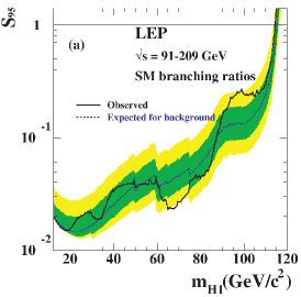
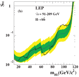
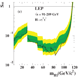
The claim of model exclusion using non-observation constraints is a statement about the statistical rejection of the “Higgs hypothesis” (i.e. that Higgs signal + background describe the data). Exclusion at the 95% C.L. means that the Higgs hypothesis has at most 5% probability. If no Higgs signal has been found, the lower the predicted signal cross section, the more probable is the Higgs hypothesis. Hence, for given mass $m_{H1}$ and search channel for the Higgs boson, one can determine a lower bound $\sigma_{\text{min}}(m_{H1})$, for cross sections above which the probability of the Higgs hypothesis stays below 5%. A model with cross section $\sigma_{\text{model}}(m_{H1})>\sigma_{\text{min}}(m_{H1})$ for the given search channel is then said to be excluded at the 95% C.L. Examples of typical (here: LEP) search results are shown in Fig. 1. Each of them assumes a particular Higgs decay pattern: (a) SM decay branching ratios, (b) 100% decay into $b\bar{b}$, and (c) 100% decay into $\tau^{+}\tau^{-}$. As the decay pattern is fixed, the limit is given on the Higgs production cross section (Higgsstrahlung) only (and normalised to the SM prediction): $S_{95}(m_{H1}):={\displaystyle\sigma^{HZ}_{\text{min}}(m_{H1})}/{\displaystyle\sigma^{HZ}_{\text{SM}}(m_{H1})}$.

For the SM result in Fig. 1(a), several individual Higgs search topologies have been combined in order to increase the sensitivity to a SM Higgs boson. Hence, the result applies only to SM-like models, i.e. models where all individual signal cross sections differ from the SM at most by the multiplication with one common proportionality factor. Fig. 1(b) and Fig. 1(c) show results for single search topologies, which can be applied to any model which predicts Higgs production via Higgsstrahlung and has a non-zero BR to $b\bar{b}$ or $\tau^{+}\tau^{-}$, respectively. If for a model which is not SM-like $\sigma^{HZ}_{\text{model}}(m_{H}){\text{BR}}_{\text{model}}(H\to b\bar{b})/\sigma^{HZ}_{\text{SM}}(m_{H1})>S_{95}^{\text{observed}}(m_{H})$ in Fig. 1(b), then the model is excluded at the 95% C.L. by this search topology.

If exclusion results on several individual search topologies are available for a given model, the question arises which one to apply in order to determine if it is excluded. Claiming exclusion of the model if at least one search topology excludes it certainly does not preserve the 95% C.L. and, therefore, should not be called exclusion. The way out is to always consider only one search result for excluding a model, but chose the analysis with the highest statistical sensitivity for that. This information is encoded in the expected limit (dashed lines in Fig. 1), the limit which would result if only background events were present in the data (obtained via Monte Carlo simulation).

2 Implementation

HiggsBounds  tests the predictions of models with arbitrary Higgs sectors against exclusion bounds obtained from LEP/Tevatron Higgs searches. It provides access to all relevant Higgs exclusion limits, including expected limits. As input, the program requires the predictions of the considered model for: the number of neutral and singly charged Higgs bosons $h_{i}$ , $m_{h_{i}}$, Higgs total widths $\Gamma_{\text{tot}}(h_{i})$, decay branching ratios BR$(h_{i}\to\ldots)$, and production cross section ratios with respect to reference values. For a given model scenario, HiggsBounds considers all implemented LEP and Tevatron analyses, checks whether they can be applied to the model considered, and returns whether the scenario is excluded at the 95% C.L. or not. There are three ways to use HiggsBounds: a command line version, a subroutine version (written in Fortran 77 and 90) a web interface.

The Tevatron and LEP cross section limits are understood to be applicable to models which do not change the signature of the background processes considerably and are usually given for a narrow-width Higgs boson. From this and other sources result some limitations on the applicability of HiggsBounds which are described in detail in [3].

Now to a crucial bit of the code, namely, how one can make a statement at the 95% C.L. while considering several search analyses in parallel. First a definition: we call an “analysis application” $X$, the application of a Higgs search analysis to a particular Higgs boson (or e.g. two Higgs bosons, if the analysis involves two of them) of the model under study with particular mass(es). To each analysis application $X$ corresponds a signal cross section prediction $\sigma(X)$ for the particular Higgs boson on which an upper limit is put by the analysis. For each $X$, HiggsBounds uses the input to calculate the quantity $Q_{\text{model}}(X)$, which is $\sigma(X)$ up to a normalisation factor. In order to ensure the correct statistical interpretation of the results, it is crucial to only consider the experimentally observed limit for one particular $X$. Therefore, HiggsBounds must first determine $X_{0}$, which is defined as the analysis application with the highest statistical sensitivity for the model point under consideration. In order to do this, the program uses the tables of expected experimental limits to obtain a quantity $Q_{\text{expec}}$ corresponding to each $X$. The analysis application with the largest value of $Q_{\text{model}}/Q_{\text{expec}}$ is chosen as $X_{0}$. The program then determines the value for $Q_{\text{obs}}(X_{0})$, using the appropriate observed limit. If ${Q_{\text{model}}(X_{0})}{Q_{\text{obs}}(X_{0})}>1$, HiggsBounds concludes that this particular parameter point is excluded at 95 % C.L.

In HiggsBounds 2.0.0, 82 Higgs search analyses have been implemented (29 from LEP and 53 from the Tevatron). With respect to HiggsBounds 1.2.0 [4], many new types of analyses have been added and several Tevatron analyses have been replaced by updated ones. The following search topologies are implemented in HiggsBounds 2.0.0. (A full list of analyses with references is given in the manual [5].)

$\bullet$ LEP neutral Higgs analyses considering the final states:
$h_{k}Z,h_{k}\to bb$ / $\tau\tau$ / anything / invisible / $\gamma\gamma$ / hadrons;  $b\bar{b}h_{k}\to b\bar{b}b\bar{b}$ / $b\bar{b}\tau\tau$ ($h_{k}$ CP even or odd) ;  $\tau\tau h_{k}\to\tau\tau\tau\tau$ ($h_{k}$ CP even or odd) ;   $h_{k}Z,h_{k}\to h_{i}h_{i},h_{i}\to bb$ / $\tau\tau$ ;  $h_{k}h_{i},\;h_{k},h_{i}\to bb$ /$\tau\tau$ ;   $h_{k}h_{i},\;h_{k}\to h_{i}h_{i},\;h_{i}\to bb$ / $\tau\tau$ ;   $h_{k}Z,h_{k}\to h_{i}h_{i},h_{i}\to bb,\tau\tau$ ;  $h_{k}h_{i},\;h_{k}\to bb,h_{i}\to\tau\tau$.

$\bullet$ Tevatron neutral Higgs single topology considering the final states:
$Zh_{k}\to llb\bar{b}$ ;  $Wh_{k}\to l\nu b\bar{b}$ ;  $bh_{k}\to 3b\text{ jets}$ ;  $\text{single }h_{k}\to WW$ ;  $\text{single }h_{k}\to\tau\tau$ ;  $Wh_{k}\to 3W$ ;  $bh_{k}\to b\tau\tau$ ;  $t\bar{t}h_{k}\to t\bar{t}b\bar{b}$ ;  $\text{single }h_{k}\to Z\gamma$.

$\bullet$ Tevatron SM Higgs combined topologies considering the final states (schematic):
$Vh_{k}\to b\bar{b}+E_{T}^{\text{miss}}(V=W,Z)$ ;   $h_{k}+X\to WW+X$ ;   $h_{k}\to WW\to ll$ ;   $h_{k}+X\to\tau\tau$ ;   $h_{k}+X\to bb+X$ ;   $Vh_{k}\to VVV\to l^{\pm}l^{\pm}+X$ ($l=e,\mu$, $V=W,Z$) ;   $h_{k}+X\to\gamma\gamma+X$;   $h_{k}+X$.

$\bullet$ LEP/Tevatron charged Higgs analyses:
$e^{+}e^{-}\to H^{+}H^{-}\to$ 4 jets ;   $e^{+}e^{-}\to H^{+}H^{-}\to\tau\nu\tau\nu$ ;   $p\bar{p}\to tt,t\to H^{+}b,\;H^{+}\to cs$ (& c.c.) ;   $p\bar{p}\to tt,t\to H^{+}b,\;H^{+}\to\tau\nu$ (& c.c.).

3 Applications

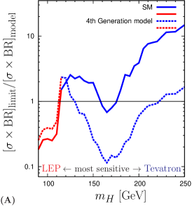
$\bullet$ 4${}^{\text{th}}$ Generation Model (FGM): As a toy example, we study a simplified FGM, where we fix $\Gamma(H\to gg)_{\text{model}}=9\,\Gamma(H\to gg)_{\text{SM}}$ for all Higgs masses . Fig. 2(A) shows the ratio of the signal cross section limit vs. the model prediction for the SM (solid) and the FGM (dashed) obtained with HiggsBounds 2.0.0. The SM curve reproduces nicely the LEP and Tevatron exclusions presented at the ICHEP’10. In the FGM, $\sigma(p\bar{p}\to gg\to H\to W^{+}W^{-})$ is strongly enhanced compared to the SM. Hence, the Tevatron Higgs mass exclusion in this model stretches from 130 GeV to 220 GeV. Given our simplified approach, this is in very good agreement with [6].

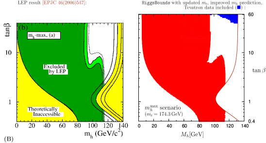
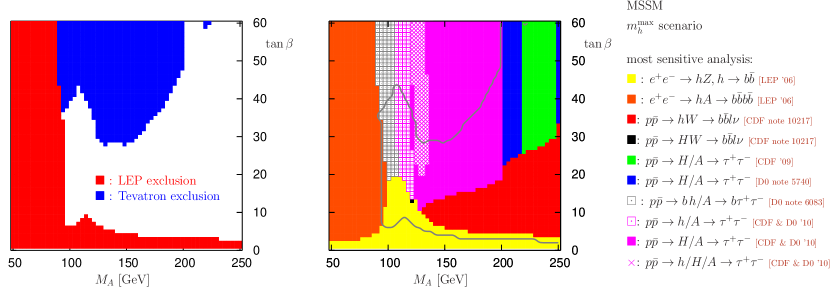
$\bullet$ MSSM Benchmark Scenarios: HiggsBounds is useful to update LEP exclusion plots for MSSM benchmark scenarios. Fig. 2(B) shows the good agreement between LEP results for the $m_{h}^{\text{max}}$ scenario [2] (left panel) and results obtained with HiggsBounds 1.0.0 (right panel) with updated MSSM predictions (using FeynHiggs 2.6.4 [7]). Verison 1.0.0 already contains all relevant LEP search channels for this comparison. Slight differences originate from the fact that HiggsBounds relies on LEP data for single topological cross sections, while the full LEP analysis combines the different search channels. Fig. 3 shows for the MSSM $m_{h}^{\text{max}}$ scenario the exclusion region (left panel) and the analyses with highest statistical sensitivity in the $m_{A}-\tan\beta$ plane obtained with HiggsBounds 2.0.0, i.e. including all Tevatron analyses presented at the ICHEP’10, and FeynHiggs 2.7.1 [7] for the model predictions. The gap in the Tevatron exclusion for $200\,\text{GeV}<m_{A}<220\,\text{GeV}$ could possibly be filled if the CDF & DØ combined $\tau\tau$ analysis [8], which has the highest sensitivity for the Tevatron exclusion for $110\,\text{GeV}<m_{A}<200\,\text{GeV}$, could be extended to values $m_{A}>200$ GeV.

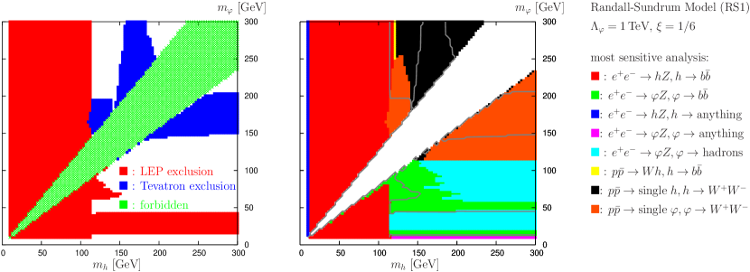
$\bullet$ Scalar Sector of the Randall-Sundrum Model: The Randall-Sundrum (RS) Model considers spacetime a slice of 5d anti-de-Sitter space with two boundaries, the IR brane (our 4d spacetime) and the UV brane [9], which naturally explains the hierarchy problem. As a consequence of stabilising the compactification “radius” in the model, an additional scalar, the radion $\varphi_{0}$, appears in the spectrum [10]. Higgs–radion mixing may occur via the interaction ${\cal L}=-\xi\sqrt{-g_{\text{ind}}}\>R(g_{\text{ind}})\>\Phi^{\dagger}\Phi$, where $g_{\text{ind}}$ is the induced 4d metric on the IR brane, $R$ the Ricci scalar, and $\Phi$ the Higgs doublet. Hence, in general, the physical Higgs $h_{0}$ and the radion $\varphi_{0}$ mix to form two mass eigenstates $h,\varphi$. Like for the Higgs, the radion couplings to massive fermions and gauge bosons are $\propto$ mass, but e.g. the couplings $\varphi_{0}\,b\bar{b}$ and $\varphi_{0}\,\gamma\gamma$ are suppressed while $\varphi_{0}\,gg$ is enhanced with respect to the SM Higgs. Although presently many modifications to the original RS Model (RS1) are considered, the RS scalar sector is a rather robust prediction, as it is closely linked to the solution of the hierarchy problem. Fig. 4 shows for RS1 the excluded region (left panel) and the search channel with highest sensitivity (right panel) in the $m_{h}-m_{\varphi}$ plane, while the two other free parameters in this model are set to $\Lambda_{\varphi}=1\,\text{TeV}$ and $\xi=1/6$. This scenario shows slight Higgs–radion mixing, i.e. $h$ behaves mainly like the SM Higgs and $\varphi$ mainly like the unmixed radion. Given the properties of $h_{0}$ and $\varphi_{0}$, this is reflected in several ways by the pattern of LEP/Tevatron exclusions and highest-sensitivity channels as a function of $m_{h}$ and $m_{\varphi}$.

4 Summary

The Higgs search at Tevatron and LEP turn(ed) out many limits on cross sections of individual and combined signal topologies. Published individually, it is no easy to make use of all of them. HiggsBounds 2.0.0 is a model-independent tool which offers easy access to a wealth of published limits in three ways: command line, subroutines, web interface. It offers a flexible range of input formats for the necessary model predictions, including the number of neutral and charged Higgs bosons. Applications to a $4^{\text{th}}$ generation model, the MSSM and the Randall-Sundrum model demonstrate its usefulness. The code is publicly available [5].

Figure 2: (A) Ratio $[\sigma\times{\text{BR}}]_{\text{obs. limit }}/[\sigma\times{\text{BR}}]_{\text{model}}$ for the most sensitive analysis as a function of the Higgs mass $m_{H}$: 4th Generation Model versus SM. (B) Excluded region in the $m_{h}-\tan\beta$ plane for the MSSM $m_{h}^{\text{max}}$ scenario. Results from LEP [2] and obtained by using HiggsBounds 1.0.0 are compared.

Figure 3: Excluded region in the $m_{A}-\tan\beta$ plane for the MSSM $m_{h}^{\text{max}}$ scenario (left panel) and most sensitive analysis (right panel) using HiggsBounds 2.0.0.

Figure 4: Excluded region in the $m_{h}-m_{\varphi}$ plane of the scalar sector of the original Randall-Sundrum model (RS1) (left panel) and most sensitive search channel (right panel) using HiggsBounds 2.0.0.

References

- [1] R. Barate et al., Phys. Lett. B 565 (2003) 61.
- [2] S. Schael et al., Eur. Phys. J. C 47 (2006) 547.
- [3] P. Bechtle, O. Brein, S. Heinemeyer, G. Weiglein and K. Williams, Comput. Phys. Commun. 181 (2010) 138.
- [4] P. Bechtle, O. Brein, S. Heinemeyer, G. Weiglein and K. Williams, AIP Conf. Proc. 1200 (2010) 510.
- [5] See: www.ippp.dur.ac.uk/HiggsBounds/.
- [6] T. Aaltonen et al., arXiv:1005.3216 [hep-ex].
- [7] S. Heinemeyer, W. Hollik, G. Weiglein, Comput. Phys. Commun. 124 (2000) 76 and Eur. Phys. J. C 9 (1999) 343; G. Degrassi, et al. Eur. Phys. J. C 28 (2003) 133; M. Frank, et al. JHEP 0702 (2007) 047.
- [8] D. Benjamin et al. [Tevatron New Phenomena & Higgs Working Group], arXiv:1003.3363 [hep-ex].
- [9] L. Randall and R. Sundrum, Phys. Rev. Lett. 83 (1999) 3370.
- [10] W. D. Goldberger and M. B. Wise, Phys. Rev. Lett. 83 (1999) 4922 and Phys. Lett. B 475 (2000) 275.