Spectra, elliptic flow and azimuthally sensitive HBT radii from Buda-Lund model for $\sqrt{s_{NN}}=200$ GeV Au+Au collisions

Abstract

We present calculations of elliptic flow and azimuthal dependence of correlation radii in the ellipsoidally symmetric generalization of the Buda-Lund hydrodynamic model of hadron production in high-energy nuclear collisions. We compare them to data from RHIC by simultaneous fits to azimuthally integrated invariant spectra of pions, kaons and protons-antiprotons measured by PHENIX in Au+Au reactions at center of mass energy of 200 AGeV. STAR data were used for azimuthally sensitive two-particle correlation function radii and for the transverse momentum dependence of the elliptic flow parameter $v_{2}$. We have found that the transverse flow is faster in the reaction plane then out of plane, which results in a reaction zone that gets slightly more elongated in-plane than out of plane. The model parameters extracted from the fits are shown and discussed.

1 Introduction

Important information about the properties of extremely hot strongly interacting matter comes from the observation of azimuthal anisotropies in non-central ultra-relativistic nuclear collisions. The second order Fourier component of azimuthal hadron distributions is connected with the azimuthal dependence of transverse collective expansion velocity of the bulk matter Heiselberg:1998es ; Sorge:1998mk . That is in turn determined by the differences of the initial pressure gradients in the two perpendicular transverse directions, as well as by the initial geometry, the initial velocity and temperature distributions of the fireball, and the equation of state Heinz:2001xi ; Csorgo:2001xm . The anisotropic shape of the fireball measured with the help of correlation femtoscopy Wiedemann:1997cr at the instant of final decoupling of hadrons bears information about the total lifespan of the hot matter: with time the originally out-of-reaction-plane shape becomes more and more round and may even become in-plane extended Heinz:2002sq . Unfortunately, in determining the elliptic flow and azimuthally sensitive correlation radii individually two effects—spatial and flow anisotropy—are entangled. For example, the same elliptic flow can be generated with varying flow anisotropy strength if the spatial anisotropy is adjusted appropriately Tomasik:2004bn .

In general, the precise way of the interplay between the two anisotropies is model dependent. It has been studied and shown to be different within the Buda-Lund model Csanad:2008af as well as the Blast Wave model Tomasik:2004bn .

In this paper we analyze for the first time azimuthally sensitive Hanbury Brown – Twiss (HBT) radii, using data from non-central heavy ion collisions within framework of the Buda-Lund model. Note that the model successfully describes data from central Au+Au collisions at RHIC, as measured by BRAHMS, PHENIX, PHOBOS, and STAR collaborations, including identified particle spectra and transverse mass dependent HBT radii as well as the pseudorapidity distributions of charged particles. The model was shown before to describe the transverse mass and pseudorapidity dependence of elliptic flow of identified particles at various energies and centralities in ref. Csanad:2005gv . The Buda-Lund model formalism for non-central collisions, including elliptic flow and azimuthal angle dependence of HBT radii has been proposed first in  Csanad:2008af . The model is defined with the help of its emission function. In order to take into account the effects of resonance decays it uses the core-halo model Csorgo:1994in . In the present study, we improve on earlier versions of the Buda-Lund model, by scrutinizing the various components using azimuthally sensitive HBT data. Eventually we utilize a model that includes as a special case of T.S. Biró ’s axially symmetric and accelerationless exact solution of relativistic hydrodynamics Biro:1999eh , in contrast to the original, earlier variant, ref. Csanad:2008af , which was based on an ellipsoidally symmetric, but also non-accelerating exact solution of relativistic hydrodynamics, given by ref. Csorgo:2003rt . Similarly to ref.  Csorgo:1999sj , we present an improved calculation, using the binary source formalism, to obtain the observables by using two saddle-points instead of only one. This results in an oscillating pre-factor in front of the Gaussian in the two-pion correlation function that we take into account for the formulae of the HBT radii.

Azimuthally sensitive HBT radii were also considered recently in cascade models, e.g. in the fast Monte-Carlo model of ref. Amelin:2007ic , or, in the Hadronic Resonance Cascade Humanic:2005ye .

Data analysis of correlation HBT radii performed earlier with the Blast Wave model indicates that the fireball at the freeze-out is elongated slightly out of the reaction plane Adams:2004yc , i.e. spatial deformation is similar as in the initial state given by the overlap function. This is also supported by the theoretical results from hydrodynamic simulations Heinz:2002sq ; Frodermann:2007ab and URQMD Lisa:2009wp . It sets limitations on the total lifespan. From all previous analyses it seems, however, that the final state anisotropy has an interesting non-monotonous dependence on collision energy with a minimum at the SPS energies Lisa:2009wp . In our analysis of the same data with a different model we observe for the first time at RHIC an in-plane elongation of the fireball at freeze-out.

The paper is structured as follows: In Section 2 the basic features of the ellipsoidally symmetric Buda-Lund model are summarized. In Section 3 we derive the analytic formulae for the observables such as elliptic flow and the azimuthally asymmetric correlation radii. In Section 4 we show the results of the simultaneous model fits to experimental data from non-central collisions and we compare them to the ones obtained from fits to central data. In Section 5 our conclusions are presented.

2 Buda-Lund model: basic features

We restrict ourselves here to a short description of the model, for details see refs. Csanad:2008af ; Csanad:2003qa .

In the Buda-Lund model, the emission function is given by that of a hydrodynamically expanding fireball (core), surrounded by a halo of long lived resonances. The core emission function looks like:

$$S_{c}(x,p)d^{4}x=\frac{g}{(2\pi)^{3}}\frac{p^{\mu}d^{4}\Sigma_{\mu}(x)}{B(x,p)+s_{q}},$$ (1)

where $g$ is the degeneracy factor ($g=1$ for identified pseudoscalar mesons, $g=2$ for identified spin=1/2 baryons), and $p^{\mu}d^{4}\Sigma_{\mu}(x)$ is a generalized Cooper-Frye term, describing the flux of particles through a distribution of layers of freeze-out hypersurfaces, $B(x,p)$ is the (inverse) Boltzmann phase-space distribution, and the term $s_{q}$ is determined by quantum statistics, $s_{q}=0$, $-1$, and $+1$ for Boltzmann, Bose-Einstein and Fermi-Dirac distributions, respectively. Note that $x^{\mu}=(t,r_{x},r_{y},r_{z})$ and $p^{\mu}=(E,p_{x},p_{y},p_{z})$ are the four-vectors of the space-time point $x$ and the momentum $p$.

For a relativistic, hydrodynamically expanding system, the (inverse) Boltzmann phase-space distribution is

$$B(x,p)=\exp\left(\frac{p\cdot u(x)}{T(x)}-\frac{\mu(x)}{T(x)}\right).$$ (2)

The forms of the flow four-velocity ($u_{\nu}(x)$), chemical potential ($\mu(x)$), and temperature ($T(x))$ distributions are introduced below. Note that it can be mapped onto exact solutions of hydrodynamics, both in the relativistic and in the non-relativistic cases, as detailed in ref.  Csanad:2003qa . For example, let us mention, that in the non-relativistic limit, the Buda-Lund hydro model corresponds to the exact, parametric, ellipsoidally symmetric solutions of non-relativistic hydrodynamics in ref. Csorgo:2001xm which solution at late times converges to an accelerationless exact solution of relativistic hydrodynamics as detailed in ref. Csorgo:2003ry . According to our best knowledge, no similar connection has been explored yet in case of the azimuthally sensitive version of the Blast Wave model of ref. Retiere:2003kf , and known exact parametric solutions of (relativistic) hydrodynamics.

The generalized Cooper-Frye pre-factor, as described in refs. Csanad:2008af ; Csanad:2003qa was

$$p^{\mu}d^{4}\Sigma_{\mu}(x)=p^{\mu}u_{\mu}(x)H(\tau)d^{4}x.$$ (3)

The time dependence of the emission, described by $H(\tau)$ was approximated with a Gaussian distribution around the freeze-out proper-time $\tau_{0}$,

$$H(\tau)=\frac{1}{(2\pi\Delta\tau^{2})^{1/2}}\exp\left(-\frac{(\tau-\tau_{0})^{2}}{2\Delta\tau^{2}}\right),$$ (4)

with $\Delta\tau$ being the duration of the particle production in longitudinal proper-time ($\tau=\sqrt{t^{2}-r_{z}^{2}}$). Of course, this function $H(\tau)$ can be easily generalized to have more complicated forms, but the data discussed in the present paper do not require us to go beyond the Gaussian approximation. However, we found that the analysis of the azimuthally sensitive HBT radii was actually sensitive to the structure of the Cooper-Frye pre-factor. Eq. (3) corresponds to freeze-out hypersurface layers that are pseudo-orthogonal to the four-velocity. For flow profiles with significant longitudinal and radial flows, as specified below, these hypersurfaces have positive correlations between the transverse radial coordinates $r_{t}$ and time $t$. When defining the axially symmetric Buda-Lund model in ref.  Csorgo:1999sj , such positive $(r_{t},t)$ correlations were neglected and the freeze-out hypersurface was assumed to be a constant in the transverse direction. Recently, new exact analytic solutions of relativistic hydrodynamics also lead to freeze-out hypersurfaces with the property of nearly negligible $(r_{t},t)$ correlations, see ref. Gubser:2010ze . Based on favourable comparisons with data and analogies to the axially symmetric Buda-Lund model, we decided to keep this kind of freeze-out hypersurfaces for the purpose of the present paper. Note also that following ref. Csorgo:1999sj of the axially symmetric case, we include a factor $\tau$ to $H_{*}(\tau)$ and approximate it by a Gaussian $H(\tau)$. Thus our modified Cooper-Frye term reads as

$$p^{\mu}d^{4}\Sigma_{\mu}(x)=m_{t}\cosh(\eta-y)H(\tau)d\tau\,\tau_{0}\,d\eta\,dr_{x}dr_{y},$$ (5)

where $m_{t}=\sqrt{m^{2}+p_{t}^{2}}$ is the transverse mass, $p_{t}$ is the transverse momentum, $y$ is the rapidity and $\eta$ is the longitudinal space-time rapidity $\eta=0.5\log[(t+r_{z})/(t-r_{z})]$. The four-velocity field, $u^{\mu}(x)$ assumed to be a directional Hubble flow, where two different radial Hubble constants ($H_{x}$ and $H_{y}$) characterize the different strength of the flow in the impact parameter plane ($x-z$) and out of this plane ($y-z$). This transverse flow is assumed to develop on a flow profile that is Bjorken-type at the $r_{t}=0$ axes of the collision :

$$u^{\mu}(x) =(\cosh[\eta]\cosh[\eta_{t}],H_{x}r_{x},H_{y}r_{y},\sinh[\eta]\cosh[\eta_{t}])$$ (6)

with $H_{x}={\dot{R}}_{x}/R_{x}$ and $H_{y}={\dot{R}}_{y}/R_{y}$ are the defining relationships for the flow in the impact parameter plane (called also as reaction plane) and in the remaining orthogonal transverse direction. $R_{x}$ and $R_{y}$ are the characteristic geometrical system sizes in the two transverse directions, whereas $\dot{R}_{x}$ and $\dot{R}_{y}$ are their time derivatives. The average transverse fluid rapidity $\eta_{t}$ is also introduced with the defining relation $\sinh^{2}[\eta_{t}]=r_{x}^{2}H_{x}^{2}+r_{y}^{2}H_{y}^{2}$, which ensures that $u\cdot u=1$. Note that at mid-rapidity, with $\eta=0$, the velocity profile of T.S. Biró ’s axially symmetric and accelerationless exact solution of relativistic hydrodynamics Biro:1999eh corresponds to the ${\dot{R}}_{x}/R_{x}={\dot{R}}_{y}/R_{y}$ case, while the solution discussed in ref.  Csorgo:2003rt coincides with this velocity profile.

For the fugacity distribution $\exp\frac{\mu(x)}{T(x)}$ we assume

$$\frac{\mu(x)}{T(x)}=\frac{\mu_{0}}{T_{0}}-\frac{r_{x}^{2}}{2R_{x}^{2}}-\frac{r_{y}^{2}}{2R_{y}^{2}}-\frac{(\eta-y_{0})^{2}}{2\Delta\eta^{2}},$$ (7)

so that it leads to a Gaussian in coordinate space. $\Delta\eta$ denotes the space-time rapidity width and $y_{0}$ is the mid-rapidity.

For the temperature profile we use the following form:

$$\frac{1}{T(x)}=\frac{1}{T_{0}}\left(1+a_{x}^{2}\frac{r_{x}^{2}}{2R_{x}^{2}}+a_{y}^{2}\frac{r_{y}^{2}}{2R_{y}^{2}}\right)\left(1+a_{\tau}^{2}\frac{(\tau-\tau_{0})^{2}}{2\Delta\tau^{2}}\right),$$ (8)

where $T_{0}$ is the temperature of the collision center at the mean freeze-out time $\tau_{0}$. The parameters $a_{x}$, $a_{y}$ and $a_{\tau}$ control the transversal and the temporal changes of the local temperature profile. Note that its dependence on the coordinate $\eta$ will not be studied here (i.e. $a_{\eta}=0$ is assumed).

3 Observables from the Buda-Lund model

The observables can be calculated analytically from the Buda-Lund hydro model, using a double saddle-point approximation in the integration. We quote results from ref. Csanad:2003qa . Note that in the binary source formalism of ref. Csorgo:1999sj (Section 8 and 9) the double saddle-points are generated from the saddle-point $\overline{x}$ of the Boltzmann term by the product with the Cooper-Frey pre-factor in which the two exponentials in the pre-factor generate two terms with separate saddle points. Hence, in the final formulae only $\overline{x}$ appears. The saddle point coordinates $\overline{x}^{\mu}=$ ($\overline{\tau}\cosh(\overline{\eta})$,$\overline{r}_{x}$,$\overline{r}_{y}$, $\overline{\tau}\sinh(\overline{\eta})$) and the longitudinally boost invariant average emission widths ($\Delta\overline{\tau}$, $\Delta\overline{\eta}$, $\overline{R}_{x}$, $\overline{R}_{y}$) are given as:

$$\overline{\tau}= \;\tau_{0},$$ (9a)

$$\overline{\eta}= \frac{y_{0}-y}{1+\Delta\eta^{2}m_{t}/T_{0}}+y,$$ (9b)

$$\overline{r}_{i}= \frac{p_{i}\dot{R}_{i}R_{i}/T_{0}}{1+(a_{i}^{2}+{\dot{R}}_{i}^{2})\overline{E}/T_{0}}\;\mathrm{for}\;i=x,y,$$ (9c)

$$\Delta\overline{\tau}^{2}= \frac{\Delta\tau^{2}}{1+a_{\tau}^{2}\overline{E}/T_{0}},$$ (9d)

$$\Delta\overline{\eta}^{2}= \frac{\Delta\eta^{2}}{1+\Delta\eta^{2}\overline{E}/T_{0}},$$ (9e)

$$\overline{R}_{i}^{2}= \frac{R_{i}^{2}}{1+(a_{i}^{2}+{\dot{R}}_{i}^{2})\overline{E}/T_{0}})\;\mathrm{for}\;i=x,y,$$ (9f)

where $\overline{E}=m_{t}\cosh(\overline{\eta}-y)$. The invariant momentum distribution is evaluated using an ellipsoidally symmetric generalization of eqs. (127, 130-140) of ref.  Csorgo:1999sj , that were first derived for the case of axially symmetric collisions:

$$E\frac{d^{3}N}{dp^{3}}={N_{1}}(p)=\frac{g}{(2\pi)^{3}}\overline{E}\;\overline{V}\;\overline{C}\;\frac{1}{B(\overline{x},p)+s_{q}},$$ (10)

where

$$\overline{V} =(2\pi)^{3/2}\,\frac{\Delta\overline{\tau}}{\Delta\tau}\,\overline{R}_{\parallel}\overline{R}_{x}\overline{R}_{y},$$ (11)

$$\overline{C} =\frac{1}{\sqrt{\lambda_{*}}}\exp(\Delta\overline{\eta}^{2}/2).$$ (12)

In the latter two expressions we use the notation $\overline{R}_{\parallel}=\tau_{0}\Delta\overline{\eta}$ and $\lambda_{*}$ is the ($y$ and $p_{t}$ dependent) intercept parameter of the two-particle correlation function.

The axially symmetric limit of these formulae, given in ref. Csorgo:1999sj corresponds to the replacements of $H_{x}=H_{y}\rightarrow H_{t}$, $a_{x}=a_{y}\rightarrow a_{r}$, $r_{x}\rightarrow r_{t}$, $r_{y}\rightarrow 0$ and $\overline{R}_{x}\overline{R}_{y}\rightarrow\overline{R}_{t}^{2}$.

The azimuthal angle ($\phi$) dependence of the invariant momentum distribution, eq. (10), can be re-expressed using a Fourier-expansion in $\phi$:

$$N_{1}(p)=N_{1}(p_{t},p_{z})\left[1+2\sum_{\begin{subarray}{c}n=1\end{subarray}}^{\infty}v_{n}\cos(n\phi)\right],$$ (13)

where $v_{n}$ are the flow coefficients, in particular $v_{2}$ is the elliptic flow. Sine terms do not appear in the expression due to mirror symmetry with respect to the reaction plane. The azimuthally averaged transverse momentum distribution $N_{1}(p_{t},p_{z})$ from $N_{1}(p)$ of eq. (10) is

$$N_{1}(p_{t},p_{z})=\frac{1}{2\pi}\int_{0}^{2\pi}N_{1}(p)d\phi$$ (14)

and the elliptic flow:

$$v_{2}(p_{t},p_{z})=\frac{\int_{0}^{2\pi}d\phi N_{1}(p)\cos(2\phi)}{\int_{0}^{2\pi}d\phi N_{1}(p)}.$$ (15)

At mid-rapidity ($p_{z}=0$), in reactions of equal-mass nuclei the terms of odd coefficients in eq. (13) disappear due to the symmetry $\phi\rightarrow\phi+\pi$. In this particular case, this observable can easily be expressed analytically if we assume that $v_{2}\gg v_{n}$ if $n\geq 4$, which we may conclude from data Adare:2010vv where $v_{4}\sim v_{2}^{2}\sim 0.01$ or smaller, hence it can be neglected. Then the formula in eq. (13) simplifies to

$$N_{1}(p_{x},p_{y},p_{z}=0)=N_{1}(p_{t})\left[1+2v_{2}\cos(2\phi)\right],$$ (16)

where $p_{t}=\sqrt{p_{x}^{2}+p_{y}^{2}}$ and $p_{x}=p_{t}\cos\phi,p_{y}=p_{t}\sin\phi$. If we evaluate this equation at two appropriate angles ($\phi=0^{o}$ and $\phi=45^{o}$) then the transverse momentum dependence of the coefficient of the elliptic flow can be re-expressed as follows

$$v_{2}(p_{t})=\frac{1}{2}\left(\frac{N_{1}(p_{t},0,0)}{N_{1}\left(\frac{p_{t}}{\sqrt{2}},\frac{p_{t}}{\sqrt{2}},0\right)}-1\right).$$ (17)

This leads to a simple analytic derivation of $v_{2}(p_{t})$ at mid-rapidity. Numerical investigations at the physical values of the model parameters indicate that the formulae have about 1% relative error, only. Note that the azimuthally averaged transverse momentum distribution in this case takes also a simple form as

$$N_{1}(p_{t})=N_{1}\left(\frac{p_{t}}{\sqrt{2}},\frac{p_{t}}{\sqrt{2}},0\right).$$ (18)

However, we can use another but less precise method, as well, to find analytic approximation for the elliptic flow. In the next procedure a scaling variable $w$ is introduced. We show that after some approximations, $v_{2}$ depends on any variable through this variable $w$ only, hence $v_{2}(w)$ is a universal function as already pointed out in refs. Csorgo:2001xm ; Csorgo:1994in ; Csanad:2003qa ; Csanad:2005gv . Both methods were tested against data but the previous one proved to describe them with better confidence.

If we evaluate $B(\overline{x},p)$ at mid-rapidity in the limit, where the saddle-point coordinates are all small, we get:

$$\ln B(\overline{x},p)=\frac{p_{x}^{2}}{2m_{t}T_{x}}+\frac{p_{y}^{2}}{2m_{t}T_{y}}-\frac{p_{t}^{2}}{2m_{t}T_{0}}+\frac{m_{t}}{T_{0}}-\frac{\mu_{0}}{T_{0}},$$ (19)

where the direction dependent slope parameters are

$$T_{x} = T_{0}+m_{t}\,{\dot{R}}_{x}^{2}\frac{T_{0}}{T_{0}+m_{t}a_{x}^{2}},$$ (20)

$$T_{y} = T_{0}+m_{t}\,{\dot{R}}_{y}^{2}\frac{T_{0}}{T_{0}+m_{t}a_{y}^{2}}.$$ (21)

The result for the (azimuthally integrated) transverse momentum spectrum is:

$$N_{1}(p_{t}) \approx \frac{g}{(2\pi)^{3}}\left[\overline{E}\overline{V}\overline{C}\right]_{p_{x}=p_{y}=p_{t}/\sqrt{2}\,\,}\exp\left[-\frac{p_{t}^{2}}{2m_{t}T_{\rm eff}}\right]$$

where we have introduced $T_{\rm eff}$, the effective slope of the azimuthally averaged single particle $p_{t}$ spectra as the harmonic mean of the slope parameters in the in-plane and in the out-of-plane transverse directions,

$$\frac{1}{T_{\rm eff}}=\frac{1}{2}\left(\frac{1}{T_{x}}+\frac{1}{T_{y}}\right)\,,$$ (23)

The result for the elliptic flow is the following simple scaling law:

$$v_{2}\cong\frac{I_{1}(w)}{I_{0}(w)},$$ (24)

where $I_{n}(z)$ stands for the modified Bessel function of the second kind, $I_{n}(z)=(1/\pi)\int_{0}^{\pi}\exp(z\cos\theta)\cos(n\theta)d\theta$. The scaling variable

$$w=\frac{p_{t}^{2}}{4m_{t}}\left(\frac{1}{T_{y}}-\frac{1}{T_{x}}\right)\,.$$ (25)

This can also be written as

$$w=E_{K}\,\frac{\epsilon}{T_{\rm eff}}\,,$$ (26)

where $E_{K}$ is a relativistic generalization of the transverse kinetic energy, defined as

$$E_{K}=\frac{p_{t}^{2}}{2m_{t}}\,,$$ (27)

and momentum space eccentricity parameter

$$\epsilon=\frac{T_{x}-T_{y}}{T_{x}+T_{y}}\,.$$ (28)

In order to compare more easily the Buda-Lund model results for the elliptic flow with the azimuthally sensitive extension of the Blast Wave model Retiere:2003kf ; Tomasik:2004bn , we introduce $\rho_{0}$ and $\rho_{2}$ so that

$${\dot{R}}_{x} =\rho_{0}(1+\rho_{2})$$ (29a)

$${\dot{R}}_{y} =\rho_{0}(1-\rho_{2})$$ (29b)

therefore

$$\rho_{0} =\frac{1}{2}\left({\dot{R}}_{x}+{\dot{R}}_{y}\right)$$ (30a)

$$\rho_{2} =\frac{{\dot{R}}_{x}-{\dot{R}}_{y}}{{\dot{R}}_{x}+{\dot{R}}_{y}}\,.$$ (30b)

The elliptic flow in the Buda-Lund model also depends on the transverse temperature gradients $a_{x}$ and $a_{y}$. The difference between them actually moderates the difference between $T_{x}$ and $T_{y}$ and modifies the elliptic flow at given $\rho_{0}$ and $\rho_{2}$. On the other hand, at larger momenta and small temperature gradient, the following approximative proportionality holds:

$$v_{2}\propto\frac{\rho_{2}}{(\rho_{2}^{2}-1)^{2}}.$$ (31)

In the following we detail the results on HBT radii. We assume that the fireball is not tilted in the reaction plane, i.e. there is no $x$-$z$ correlation in the emission points of the hadrons. There is, however, an angle $\varphi$ between the main axis of the ellipsoidal cross-section of the fireball and the outward and sideward axes given by the momentum of the hadrons. The former are determined by the orientation of the reaction plane while the latter are defined so that the outward axis agrees with the direction of the average transverse momentum of the pair and the sideward axis is perpendicular to it. Following eq. (128) in ref. Csorgo:1999sj , the formula for the two-particle Bose-Einstein correlation function can be expressed as

$$C_{2}({\bf k_{1},k_{2}})=\frac{N_{2}(\bf k_{1},k_{2})}{N_{1}({\bf k_{1}})N_{1}(\bf k_{2})}=1+\lambda_{*}\Omega(q_{\parallel})\exp(-q_{i}^{2}\overline{R}_{i}^{2}),\\$$ (32)

where $q=k_{1}-k_{2}=(q_{=},q_{\parallel},q_{x},q_{y})$, $\overline{R}=(\Delta\tau,\overline{R}_{\parallel},\overline{R}_{x},\overline{R}_{y})$ and in the exponential we use the Einstein summation rule over the same indices. The longitudinally boost invariant $temporal$, $parallel$, $side$ward, $out$ward relative momentum components are defined as

$$q_{=}\, =\,q_{0}\cosh(\overline{\eta})-q_{z}\sinh(\overline{\eta}),$$ (33a)

$$q_{\parallel}\, =\,q_{z}\cosh(\overline{\eta})-q_{0}\sinh(\overline{\eta}),$$ (33b)

$$q_{out}\, =\,(q_{x}K_{y}-q_{y}K_{x})/\sqrt{K_{x}^{2}+K_{y}^{2}},$$ (33c)

$$q_{side}\, =\,(q_{x}K_{x}+q_{y}K_{y})/\sqrt{K_{x}^{2}+K_{y}^{2}},$$ (33d)

$$Q^{2} =-q^{\mu}q_{\mu}\,=-q_{=}^{2}+q_{\parallel}^{2}+q_{x}^{2}+q_{y}^{2}$$ (33e)

$$=-q_{=}^{2}+q_{\parallel}^{2}+q_{side}^{2}+q_{out}^{2},$$ (33f)

where $K=0.5(k_{1}+k_{2})$. The pre-factor $\Omega$ induces oscillations within the Gaussian envelope as a function of $q_{\parallel}$. This factor is given as

$$\Omega(q_{\parallel})=\cos^{2}(q_{\parallel}\overline{R}_{\parallel}\Delta\overline{\eta})+\sin^{2}(q_{\parallel}\overline{R}_{\parallel}\Delta\overline{\eta})\tanh^{2}(\overline{\eta}).$$ (34)

However, it can be approximated by a Gaussian, too, hence we may merge it with the longitudinal and temporal emission widths as:

$$\overline{R}_{\parallel,G}^{2} =R_{\parallel}^{2}(1+\Delta\overline{\eta}^{2}/\cosh^{2}(\overline{\eta})),$$ (35a)

$$\Delta\overline{\tau}_{G}^{2} =\sinh^{2}(\overline{\eta})R_{\parallel,G}^{2}+\cosh^{2}(\overline{\eta})\Delta\overline{\tau}^{2}.$$ (35b)

A widely used parameterization of the correlation function is given in the longitudinally co-moving frame (LCMS Csorgo:1991kfki , $\beta_{l}=0$) of the particle pair and in the out-side-long system Bertsch:1988db of Bertsch-Pratt (where $K_{\mu}=(K_{0},K_{out},0,0)$):

$$C_{2}({\bf k_{1},k_{2}})\simeq 1+\lambda_{*}\exp(-q_{i}q_{j}R_{ij}^{2}),$$ (36)

where $i,j=(out,side,long)=(o,s,l)$. Then the formulae for these HBT radii can be expressed by the following transformations

$$R_{o}^{2} =\overline{R}_{x}^{2}\cos^{2}\varphi+\overline{R}_{y}^{2}\sin^{2}\varphi+\beta_{o}^{2}\Delta\overline{\tau}_{G}^{2}$$ (37a)

$$=\frac{\overline{R}_{x}^{2}+\overline{R}_{y}^{2}}{2}+\beta_{o}^{2}\Delta\overline{\tau}_{G}^{2}-\frac{\overline{R}_{y}^{2}-\overline{R}_{x}^{2}}{2}\cos(2\varphi)\,$$

$$R_{s}^{2} =\overline{R}_{x}^{2}\sin^{2}\varphi+\overline{R}_{y}^{2}\cos^{2}\varphi$$ (37b)

$$=\frac{\overline{R}_{x}^{2}+\overline{R}_{y}^{2}}{2}+\frac{\overline{R}_{y}^{2}-\overline{R}_{x}^{2}}{2}\cos(2\varphi)\,,$$

$$R_{os}^{2} =\frac{\overline{R}_{y}^{2}-\overline{R}_{x}^{2}}{2}\sin(2\varphi)\,,$$ (37c)

$$R_{l}^{2} =\cosh^{2}(\overline{\eta})\overline{R}_{\parallel,G}^{2}+\sinh^{2}(\overline{\eta})\Delta\overline{\tau}^{2}\,,$$ (37d)

$$R_{ol}^{2} =-\beta_{o}\sinh(\overline{\eta})\cosh(\overline{\eta})(\overline{R}_{\parallel}^{2}+\Delta\overline{\tau}^{2})\,,$$ (37e)

$$R_{sl}^{2} =0\,.$$ (37f)

4 Comparison to experimental data

We have determined the best parameter values by fitting the analytic expressions for the observables, given in the previous section, to experimental data, with the help of the CERN Minuit fitting package. Data from 20-30% centrality class of 200 AGeV Au+Au collisions provided by PHENIX Adler:2003cb ; Adler:2004rq and STAR Adams:2004bi ; Adams:2003ra were used in the analysis. The fits were performed simultaneously to azimuthally integrated transverse mass spectra of positive and negative pions, kaons, and (anti)protons Adler:2003cb , the transverse momentum dependence of the elliptic flow parameter $v_{2}$ of pions Adams:2004bi and to the HBT radii due to pion correlations as functions of transverse mass and the azimuthal angle Adams:2003ra . The results are plotted in Figs. 1-5.

The interpretation of the model parameters is summarized in Table 1. However, for a better understanding the results three alternative parameters are introduced that can be expressed from the previous ones the following way:

$$R_{sx}^{2} =\frac{2R_{x}^{2}}{a_{x}^{2}}$$ (38a)

$$R_{sy}^{2} =\frac{2R_{y}^{2}}{a_{y}^{2}}$$ (38b)

$$T_{e} =\frac{T_{0}}{1+a_{\tau}^{2}}.$$ (38c)

The two radii parameters correspond to the thermal surface sizes where the temperature drops to $T_{0}/2$, and the parameter $T_{e}$ corresponds to the temperature of the center after most of the particle emission is over (cooling due to evaporation an expansion). Sudden emission corresponds to $T_{e}=T_{0}$, and the $\Delta\tau\rightarrow 0$ limit. Also note that we use $\mu_{B}$, baryochemical potential. This is calculated from the chemical potential of protons and antiprotons: $\mu_{B}=1/2\ (\mu_{0,p}-\mu_{0,\overline{p}})$, as written in Table 1.

In Table 2, we present the model parameters obtained from simultaneous fits to the data sets. For comparison, results are shown from our earlier analysis of 0-30% centrality collisions Csanad:2004mm , too, that was performed with a previous version of the model corresponding to the axially symmetric limit of the current ellipsoidally generalized Buda-Lund hydrodynamic model.

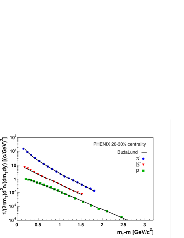
Figure 1: Buda-Lund model fits to RHIC 200GeV Au+Au data of azimuthally integrated transverse momentum spectra of negatively charged particles data Adler:2003cb .

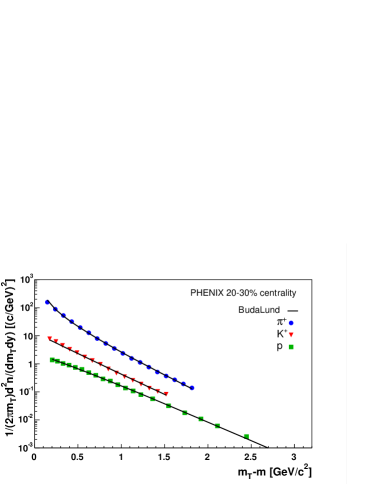
Figure 2: Buda-Lund model fits to RHIC 200GeV Au+Au data of azimuthally integrated transverse momentum spectra of positively charged particles Adler:2003cb .

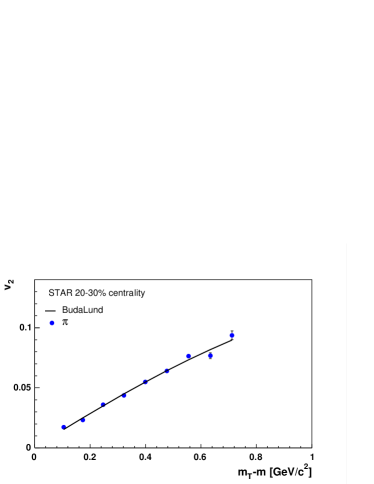
Figure 3: Buda-Lund model fit to RHIC 200GeV Au+Au data on $v_{2}$ elliptic flow of pions Adams:2004bi .

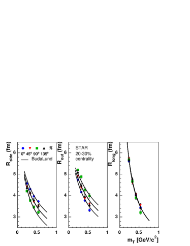
Figure 4: Buda-Lund model fits to RHIC 200GeV Au+Au data Adams:2003ra of HBT radii as a function of transverse mass for different azimuthal angles.

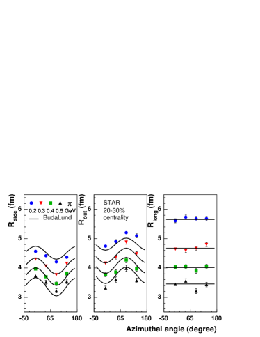
Figure 5: Buda-Lund model fits to RHIC 200GeV Au+Au data Adams:2003ra of HBT radii as functions of azimuthal angles for different values of transverse mass.

Buda-Lund	parameter description
parameters
$T_{0}$	Temperature in the center
$a_{\tau}$	Temperature gradient in proper time $\tau$
$a_{x}$	Temperature gradient in direction $x$
$a_{y}$	Temperature gradient in direction $y$
$\Delta\tau$	Distribution width in proper-time $\tau$
$\Delta\eta$	Distribution width in space-time rapidity $\eta$
$R_{x}$	Geometrical size in direction $x$
$R_{y}$	Geometrical size in direction $y$
$H_{x}$	Expansion strength in direction $x$
$H_{y}$	Expansion strength in direction $y$
$\tau_{0}$	Mean freeze-out proper-time
$\mu_{B}$	Baryochemical potential, $1/2\ (\mu_{0,p}-\mu_{0,\overline{p}})$

Table 1: Description of the parameters of the model. The values are meant at the mean freeze-out propoer-time $\tau_{0}$.

Buda-Lund	Au+Au 200 GeV		Au+Au 200 GeV
parameters	central (0-30%)		non-central (20-30%)
$T_{0}$ [MeV]	196	$\pm$ 13	174	$\pm$ 6
$T_{e}$ [MeV]	117	$\pm$ 11	130	$\pm$ 6
$\mu_{B}$ [MeV]	31	$\pm$ 28	27	$\pm$ 16
$R_{x}$ [fm]	13.5	$\pm$ 1.7	9.5	$\pm$ 0.5
$R_{y}$ [fm]	$R_{x}$		7.0	$\pm$ 0.2
$R_{sx}$ [fm]	12.4	$\pm$ 1.6	12.8	$\pm$ 0.8
$R_{sy}$ [fm]	$R_{sx}$		16.9	$\pm$ 1.6
$H_{x}$	0.119	$\pm$ 0.020	0.158	$\pm$ 0.002
$H_{y}$	$H_{x}$		0.118	$\pm$ 0.002
$\tau_{0}$ [fm/c]	5.8	$\pm$ 0.3	5.4	$\pm$ 0.1
$\Delta\tau$ [fm/c]	0.9	$\pm$ 1.2	2.5	$\pm$ 0.2
$\Delta\eta$	3.1	$\pm$ 0.1	2.5	$\pm$ 0.3
$\chi^{2}/$NDF	114/208 = 0.55		269.4/152 = $1.77$

Table 2: Source parameters from simultaneous fits to PHENIX and STAR data of Au+Au collisions at $\sqrt{s_{NN}}=200$ GeV, as given in Fig. 1-5, obtained by the Buda-Lund model. For non-central data the value of $\chi^{2}$/NDF refers to fits with statistical errors, only.

The general observation is that the Buda-Lund model parameters describing the source of non-central reactions are usually slightly smaller then those of more central collisions. However, the changes are usually within 2 standard deviations, therefore the above statement is based on the tendency of the parameters, and on some lower energy results not shown here but presented in ref. Csanad:2004mm , too. For example, the central temperature in these particular non-central reactions is below that of the more central ones. Also, the transverse geometrical radii at the mean emission time are considerably smaller compared to the more central values. Moreover, the geometric shape evolution due to the asymmetric particle transverse flow in-plane (x) an out-of-plane (y) directions results in a source more elongated in-plane. Due to the smaller longitudinal source size, the parameter corresponding to the formation of hydrodynamic phase is about 10%  smaller than that in more central collisions, $\tau_{0}(20-30\%)=5.4\pm 0.1$ fm/$c$. The elongation in longitudinal direction is similarly smaller, $\Delta\eta(20-30\%)=2.5\pm 0.3$. In both cases the baryochemical potential is found to be at a low level with respect to the proton mass. We emphasize again that the observations are based on all the fit results in ref. Csanad:2004mm .

Note that some of the azimuthally sensitive data have large systematic errors that affect the success of fits which we had to take into account. The reason for that is the difficulty of precise determination of the event reaction plane the data are relative to. Several methods are used by the experiments to overcome it and we mention those applied for the selected data.

The data set we used for fitting $v_{2}$ was calculated by the four-particle cumulants reaction plane determination method that is based on calculations of $N$-particle correlations and non-flow effects subtracted to first order when $N$ is greater than 2. The higher $N$ is the more precise the event plane determination is, as expected. STAR published two-particle cumulants $v_{2}$ data in the same reference, too, but because of the visible deviations between the two kinds of data sets and with respect to the comments above we used $v_{2}\{4\}$ data, only. For further details, see ref. Adams:2004bi .

In case of azimuthally sensitive correlation radii, STAR has cast about 10% possible systematic errors on the data on average. The most likely deviations were assumed to take effect on the ’side’ and ’out’ radii of transverse momentum of 0.2 GeV/$c$. The $\chi^{2}$/NDF for the full fit, including HBT radii with their statistical errors is 269.6/152, which corresponds to a very low confidence level. But, when we tested our fits with the above mentioned two radii of ’side’ and ’out’ of transverse momentum of 0.2 GeV/$c$ shifting them within their systematic errors (about $\pm$ 5%) we could achieve an acceptable 1% confidence level for the full simultaneous fit. However, without the contribution of the HBT radii to $\chi^{2}$/NDF the confidence level is of an acceptable level of 5.1%.

For comparison to results in refs. Retiere:2003kf ; Tomasik:2004bn of the azimuthally sensitive extension of the Blast Wave model, we have calculated the derivative values given in eqs. (30a, 30b) as $\rho_{0}=1.16\pm 0.05$ and $\rho_{2}=0.29\pm 0.02$.

5 Conclusions

We have presented the extension of the Buda-Lund hydrodynamic model from central ultra-relativistic heavy ion collisions to peripheral ones. Spectra and the elliptic flow of identified particles have been described along with the azimuthal dependence of two-particle correlation function radii in the ellipsoidally symmetric generalization of the model. Theoretical predictions were tested against RHIC data. From model fits to data of 20-30% centrality class at mid-rapidity source parameters characterizing these non-central ultra-relativistic heavy ion reactions were extracted.

The results of our analysis indicate that the central temperature in 20-30% centrality reactions is lower than that in more central collisions, $T_{0}=174\pm 6$ (stat) MeV. In an earlier analysis we showed that in more central (0-30%) reactions of the same collision energy this value was $T_{0}=196\pm 13$ (stat) MeV. We have found that the transverse flow is stronger in the reaction plane than out of plane with Hubble constants $H_{x}=0.158\pm 0.002$ and $H_{y}=0.118\pm 0.002$. The almond shape of the reaction zone initially elongated out of plane gets slightly elongated in the direction of the impact parameter by the time the particle emission rate reaches its maximum. The effect is reflected by the geometrical radii in the two perpendicular directions at that time, $R_{x}(\mathrm{in-plane})=9.5\pm 0.5$ (stat) fm, $R_{y}(\mathrm{out-plane})=7.0\pm 0.2$ (stat) fm. This is the first time that an in-plane extended source has been reconstructed from simultaneous hydrodynamic model fits to identified particle spectra, elliptic flow and azimuthally sensitive HBT data in 200 AGeV Au+Au collisions at RHIC.

The qualitative agreement between model and data is apparently good as can be judged from the figures. Although, in these fits data were used with statistical errors, only, which resulted in $\chi^{2}/$NDF$=1.77$.

Acknowledgments

Inspiring discussions with professors R. J. Glauber at Harvard University and Mike Lisa at the WPCF 2009 conference at CERN are gratefully acknowledged. This paper was prepared within a bilateral collaboration between Hungary and Slovakia under project Nos. SK-20/2006 (HU), SK-MAD-02906 (SK). B.T. acknowledges support by MSM 6840770039 and LC 07048 (Czech Republic). M.Cs., T.Cs. and A.S. gratefully acknowledge the support of the Hungarian OTKA grants T49466 and NK 73143. T. Cs. was supported also by a Senior Leaders and Scholars Fellowship of the Hungarian American Enterprise Scholarship Fund.

References

- (1) H. Heiselberg and A.-M. Levy, Phys. Rev. C59, 2716 (1999).
- (2) H. Sorge, Phys. Rev. Lett. 82, 2048 (1999).
- (3) U. W. Heinz and P. F. Kolb, Nucl. Phys. A702, 269 (2002).
- (4) T. Csörgő et al., Phys. Rev. C67, 034904 (2003).
- (5) U. A. Wiedemann, Phys. Rev. C57, 266 (1998).
- (6) U. W. Heinz and P. F. Kolb, Phys. Lett. B542, 216 (2002).
- (7) B. Tomášik, Acta Phys. Polon. B36, 2087 (2005).
- (8) M. Csanád et al., Eur. Phys. J. A38, 363 (2008).
- (9) M. Csanád, B. Tomášik, and T. Csörgő, Eur. Phys. J. A 37, 111 (2008).
- (10) T. Csörgő, B. Lörstad, and J. Zimányi, Z. Phys. C71, 491 (1996).
- (11) T. S. Bíró, Phys. Lett. B474, 21 (2000).
- (12) T. Csörgő, F. Grassi, Y. Hama, and T. Kodama, Phys. Lett. B565, 107 (2003).
- (13) T. Csörgő, Heavy Ion Phys. 15, 1 (2002).
- (14) T. Csörgő & S. Pratt, preprint-KFKI-1991-28/A, p75, (1991).
- (15) N. S. Amelin et al., Phys. Rev. C77, 014903 (2008).
- (16) T. J. Humanic, Int. J. Mod. Phys. E15, 197 (2006).
- (17) J. Adams et al., Phys. Rev. C71, 044906 (2005).
- (18) E. Frodermann, R. Chatterjee, and U. Heinz, J. Phys. G34, 2249 (2007).
- (19) M. Lisa, Talk presented at 5th Workshop on Particle Correlations and Femtoscopy, CERN, October 14-17, 2009.
- (20) M. Csanád, T. Csörgő, and B. Lörstad, Nucl. Phys. A742, 80 (2004).
- (21) T. Csörgő, L. P. Csernai, Y. Hama, and T. Kodama, Heavy Ion Phys. A21, 73 (2004).
- (22) F. Retiere and M. A. Lisa, Phys. Rev. C70, 044907 (2004).
- (23) S. S. Gubser, [arXiv:1006.0006].
- (24) A. Adare et al., Phys. Rev. Lett. 105, 062301 (2010).
- (25) G. Bertsch, M. Gong, and M. Tohyama, Phys. Rev. C37, 1896 (1988).
- (26) S. S. Adler et al., Phys. Rev. C69, 034909 (2004).
- (27) S. S. Adler et al., Phys. Rev. Lett. 93, 152302 (2004).
- (28) J. Adams et al., Phys. Rev. C72, 014904 (2005).
- (29) J. Adams et al., Phys. Rev. Lett. 93, 012301 (2004).
- (30) M. Csanád, T. Csörgő, B. Lörstad, and A. Ster, J. Phys. G30, S1079 (2004).