ON CHROMOSPHERIC VARIATIONS MODELING FOR

MAIN-SEQUENCE STARS OF G AND K SPECTRAL CLASSES

E.A.Bruevich

Sternberg Astronomical Institute, Moscow, Russia

E-mail: red-field@yandex.ru

We present a method of chromospheric flux simulation for 13 late-type main-sequence stars. These Sun-like stars have well-determined cyclic flux variations similar to $11$ yr solar activity cycle. Our flux prediction is based on chromospheric $HK$ emission time series measurements from Mount Wilson Observatory and comparable solar data. We show that solar three - component modeling explains well the stellar observations. We find that the $10-20\%$ of K - stars disc surfaces are occupied by bright active regions.

KEY WORDS: late-type stars, chromospheric variations, modeling of chromospheric emission.

1 INTRODUCTION

This paper continues the study of variability among Sun-like stars. Here the purpose is to obtain the possibility of modeling the behavior of the star’s chromospheric emission in future or for periods of time without measurements.

Observations of chromospheric variability requires at least a decade to reveal variations with timescales to the $11$ yr solar cycle.

We use the data from the observation program that was initiated by Wilson who discovered the widespread occurrence of activity cycles by monitoring $CaII$ $H$ and $K$ variations in 91 stars on or near the lower main sequence over $12$ year (Wilson, 1978). Two sets of measurements (named ”HK-project”) have been combined to make more than 30 years records of stellar chromospheric activity. Wilson made observations from 1966 to 1977 at monthly intervals on 2.5 m telescope at Mount Wilson Observatory. The survey moved in 1977 to 1.5 m telescope with instrument whose measurements can be compared to those of Wilson’s system. Some new stars were added to 91 Wilson’s stars to bring the total in the monitoring program to 111 stars (Baliunas et al., 1995). $CaII$ $H$(396.8nm) and $K$ (393.4nm) emission is observed in stars later than approximately $F2V$, i.e. less massive than about $1.5M_{\odot}$. Areas of concentrated magnetic fields on the Sun and Sun-like stars emit $CaII$ $H$ and $K$ more intensely than areas with less magnetic field present. So the contrast of Active Regions (AR) emission (where the local magnetic fields are more then some orders higher than average global magnetic field) in these $CaII$ lines changes from $1.2$ to $1.5$ with changing of chromospheric activity cycle phase.

Comparing of variability of $H$ and $K$ emission in main-sequence stars should provide important validation for theories of magnetic activity, as well as place of solar activity in a general perspective.

The influence of photospheric flux in the total solar or stars irradiance we can interpretate as the cyclic flux variations caused by slight imbalance between the flux deficit produced by dark sunspots and the excess flux produced by bright faculae.

Besides of such structures as AR in solar and stars chromosphere there is another regular structure -”chromospheric network” (connecting with the supegranulation). It also varies its own relative brightness with chromospheric activity cycle.

We can note that the maximum amplitude of photospheric flux variability in $11$ yr solar cycle may be as much as $1-3\%$ of the average photospheric flux level but the maximum amplitude of $CaII$ chromospheric flux may be as much as $20\%$ of the average level. These values are our some estimations for the maximum amplitudes of 11 yr variations of Sun-like stars photospheric and chromospheric fluxes.

2 THE THREE-COMPONENT MODEL OF STELLAR CHROMOSPHERIC EMISSION AS ANALOG OF TREE-COMPONENT MODEL OF SOLAR CHROMOSPHERIC EMISSION

The processes in solar atmosphere caused the emission in different spectral intervals and lines are studied well enough. But it’s very difficult to take into account the contribution of all different structures that emitted from the solar surface. As a successful example of solar flux model calculations in spectral intervals of $40-140$ nm (that are in agreement with SKYLAB’s observations) we can point out the (Vernazza et al., 1981).

The Vernazza’s calculations take into account the influence of 6 main different components on the solar surface and their contributions to the total emission in this spectral interval. These components are: the dark areas inside the chromospheric network cells, the centers of networks, the areas of quiet Sun, the average level of network emission region, the bright areas of network, the most bright areas of network. When the observations are not made with high accuracy all this structures we see as quiet Sun average emission (that varies with 11 yr chromospheric cycle).

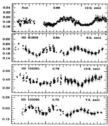
Figure 1: Records of relative CaII emission fluxes (S-index) from Mount Wilson observations (Baliunas et al.) for stars of ”EXELLENT” class for 30 years from 1965 to 1995. HD numbers of stars and their (B-V) values are presented

These structures contribute significantly to the full flux emitted from the quiet Sun chromospheric average emission.

The next most important source of solar chromosphere emission is the Active Regions (AR) emission. The SKYLAB’s observations show the brightness of AR are $1.5-2.5$ times greater the average quiet surface brightness (Schriver et al., 1985). This AR brightness contrast is depend of wavelengths. They note also that the AR surface brightness depends of the AR area and the number of spots the AR consists of.

Lean’s three-component model (that’s made for $40-140$ nm spectral interval) based on NIMBUS 7 observations (Lean et al., 1983) assumed that the full flux from chromosphere is determined by three main components.

These components are: (1) - the constant component with uniform distributed sources on solar surface, (2) - the ”active” network component (uniformly distributed too but also connected with destroyed parts of previous AR and so is proportional to total AR areas), (3) - the AR component.

So one can use Lean’s formulae for calculation of the flux in chromospheric lines:

$$I=I_{\lambda Q}\Big{\{}1+f_{N}\Big{(}C_{\lambda N}-1\Big{)}\Big{\}}+2\pi F_{\lambda Q}(1)\Sigma{A_{i}\mu_{i}R_{\lambda}(\mu_{i})}\Big{(}C_{p\lambda}W_{i}-1\Big{)}$$

where $I$ is the full flux of chromospheric emission, $I_{\lambda Q}$ is the contribution of the constant component (BASAL), $C_{p\lambda}$ is the values of AR contrasts and they are similar to contrasts from (Cook et all., 1980), $C_{N\lambda}$ is the value of ”active network” contrast: they are equal to $0.5\cdot C_{p\lambda}$ for continuum and $1/3\cdot C_{p\lambda}$ for lines, $f_{N}$ is part of disk (without AR) that is occupied by the ”active network”.

The second member in the right part of (1) describes emission from all AR on the disk; $A_{i}$ are values of their squares, $\mu_{i}$ describes the AR position: $\mu_{i}={cos{\phi_{i}}cos{\theta_{i}}}$ (where $\phi_{i}$ and $\theta_{i}$ are the coordinates of AR number $i$). $R_{\lambda}(\mu_{i})$ describes the relative change of the surface brightness $F_{\lambda Q}(\mu_{i})$ with moving from center to edge of disk. The relative adding AR contribution to full flux from the different AR is determined by the factor $W_{i}$ that is linearly changed from the value $0.76$ to $1.6$ depending of the brightness ball of flocculae (according to ball flocculae changes from $1$ to $5$).

So the ”active” network part in all the surface without AR is determined by the AR decay, the next relationship between $f_{N}$ in time moment $t$ and average values $A_{i}$ in earlier time is right:

$$f_{N}(t)=13.3\cdot 10^{-5}\cdot<\Sigma A_{i}(t-27)>$$

where the time-averaging is taken for $7$ previous rotation periods, $A_{i}$ is measured in one million parts of the disk.

To analyzed the $H$ and $K$ $CaII$ flux long-time variations in case of Sun-like stars we assume that full flux $S_{CaII}(t)$ is consists of three main components:

(1) - the”constant part” (so-called BASAL in solar physics - we call this component $P_{min}$),

(2) - the ”low-changed phone” (we call this component $P_{CaII}(t)$ ) and

(3) - ”active regions” on the disk of star (we call this component $S_{AR}(t)$).

So the full flux will be

$$S_{CaII}(t)=P_{CaII}(t)+S_{AR}(t)$$

The component (2) $P_{CaII}(t)$ consists of constant BASAL component $P_{min}$ and low-changed pseudo-sinusitis component which we can see from the Sun observations and will describe it’s approximation later.

It’s evident (from solar observations and their interpretations) that between the values $S_{CaII}(t)$ and $P_{CaII}(t)$ there is close connection.

According to (Borovik et al., 1997) the average amplitude of flux variations may be $20\%$ in maximum phase of chromospheric cycle.

This point of view is according well enough with Lean’s model (Lean et al., 1983) for solar $L_{\alpha}$ line (in case of solar $L_{\alpha}$ line flux the maximum amplitude of this flux variation in different $11$ yr cycles reached the value of $20\%$).

Than we determine the analog coefficient $k$ for star’s chromospheric cycle as equal to ratio of maximum amplitude of so called ”phone” component to maximum amplitude of full flux in long-term activity cycle:

$$k=(P_{CaII}^{max}-P_{min})/(S_{CaII}^{max}-P_{min})$$

We consider that $k$ is constant ratio between $P_{CaII}(t)$ and $S_{CaII}(t)$ for all moments during star’s cycle.

We also assume that $P_{CaII}^{max}=1.2\ P_{min}$.

It’s evident from our previous consideration that $P_{min}$ is a constant value during all long-term cycles but differs for different stars and Sun. Most likely that the value $P_{min}$ characterizes the average level of outer atmosphere activity of stars and may correlate with ROSAT observations of their X-ray fluxes (X-ray luminosity are observed on ROSAT for $65\%$ ”HK-project” stars only).

According to these we connect the full flux value $S_{CaII}(t)$ and ”phone” flux value $P_{CaII}(t)$ by analog coefficient $k$ (3):

$$P_{CaII}(t)=k\cdot S_{CaII}(t)$$

The $S_{CaII}(t)$ values we may take from observations (Baliunas et al., 1995).

At Fig 1. we can see records of relative $CaII$ $H+K$ emission fluxes ($S_{CaII}$) for 4 from 13 stars of EXCELLENT Baliunas’s class and Sun for 30 years from 1965 to 1995. Also at Fig 1. we can see HD numbers of stars and their (B - V) values.

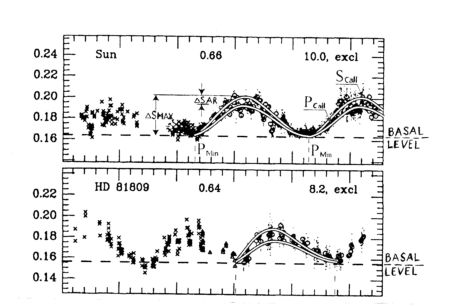
Figure 2: For Sun and HD 81809 we show BASAL level and other components for (3) - (5) equations

It’s evident (from solar observations in different spectral intervals) that $P_{CaII}(t)$ and $S_{CaII}(t)$ have similar behavior in chromospheric cycle. We’ve calculated the regression coefficients (see Table) $a$ and $b$ for the regression relation:

$$S_{CaII}(t)=a\cdot P_{CaII}(t)+b$$

To make ”phone” flux prediction we use the method from (Bocharova et al., 1983) for solar ”phone” flux variations in 11 yr cycle. Using Bocharova’s considerations we’ve obtained the next approximation for ”phone” flux $P_{CaII}(t)$ (Bruevich , 1999):

$$P_{CaII}(t)=P_{min}\cdot\Big{(}1+sin^{4}\cdot{{\pi\cdot t}\over{T}}\Big{)}\cdot e^{-{{\pi\cdot t}\over{T}}}$$

where $P_{min}$ is the minimum value of ”phone” flux is equal to BASAL flux. It corresponds to the minimum ”phone” flux value for the star and it’s constant for all observed long-term cycles, see Fig 2.

$T$ is the period of long-term chromospheric cycle calculated by (Baliunas et al.), $t$ is the time expressed in parts of period $T$:

$$t=0.1\cdot T,0.2\cdot T,...$$

So we have two methods of ”phone” flux calculations: (1) - from observations records using equations (3) and (4) (see Fig 2.), (2) - from analytic approximation (6)using $P_{min}$ only. Note that the both methods give us very identifiable values of $P_{CaII}(t)$ which differ some percents only.

So if we want the chromospheric flux to predict we may calculate $S_{CaII}(t)$ with help of equation (5) using $a$ and $b$ coefficients which are calculated earlier with help of standard regression methods and presented in Table.

In Table we present also the relative full flux variation in activity cycle maximum: (${\Delta S_{CaII}^{max}}/{P_{min}}$) and relative AR adding flux in activity cycle maximum: ($\Delta S_{AR}^{max}/P_{min}$).

These values of flux variations are presented in % of $P_{mim}$. The value $P_{mim}$ - that is equal to BASAL emission for different stars which we can determine from Baliunas’s data (Fig 1.).

Table

Object	B - V	$T_{cyc}$, yr	$P_{mim}$	a	b	${\Delta S_{CaII}^{max}}/{P_{min}}$	$\Delta S_{AR}^{max}/P_{min}$
Sun	0.66	10	0.162	1.19	-0.031	23.4	3.4
HD 81809	0.64	8.2	0.155	1.13	-0.020	22.6	2.6
HD 152391	0.76	10.9	0.32	1.56	-0.180	31.6	11.3
HD 103095	0.75	7.3	0.17	1.23	-0.040	24.7	4.7
HD 184144	0.80	7.0	0.19	1.45	-0.085	28.9	8.9
HD 26965	0.82	10.1	0.18	1.39	-0.07	27.8	7.8
HD 10476	0.84	9.4	0.17	1.61	-0.104	32.4	12.3
HD 166620	0.87	15.8	0.175	1.43	-0.075	28.6	8.6
HD 160346	0.96	7.0	0.24	1.88	-0.21	37.5	17.5
HD 4628	0.88	8.4	0.19	1.96	-0.183	39.4	19.4
HD 16160	0.98	13.2	0.19	1.61	-0.116	32.6	12.6
HD 219834B	0.91	10.0	0.17	1.92	-0.157	38.2	18.2
HD 201091	1.18	7.3	0.51	1.85	-0.434	37.2	17.2
HD 32147	1.06	11.1	0.22	1.67	-0.147	45.4	25.4

The Table data we may employed in our full flux chromospheric predictions: for the certain moment $t$ ( $t$ is the time expressed in parts of period value $T$) we can calculated the value $P_{CaII}(t)$ from equation (6). Then from equation (5) for moments $t$ and for $P_{min}$ star’s values we can calculate the predicted flux $S_{CaII}(t)$.

3 SUMMARY AND CONCLUSIONS

When we analyze results of our predictions (in Table we presented the observed values that we’re discussed in this issue and our estimations as ${\Delta S_{CaII}^{max}}/{P_{min}}$ and $\Delta S_{AR}^{max}/P_{min}$) some conclusions can be made:

K-stars of $EXELLENT$ class as Baliunas determined for stars with the most evident determination of chromospheric activity cycle (Baliunas et al.) have enough number of Active Regions at stars surfaces and these AR can emit the addition flux near $10-20\%$ of full flux in chromospheric cycle maximum, see Table. So we can see that in K-stars the most bright flocculae (its flux is two times brighter than the average chromosphere flux) may occupy almost $10-20\%$ of star’s disk.

This $10-20\%$ of AR additional flux (”phone” flux evaluation) we show in Fig 2. Also we see the star’s ”phone” flux (smoothly changed in chromospheric cycle) and BASAL component (constant in chromospheric cycle).

Note that all our three components we can see in Fig 1. (”HK-project” observations of EXCELLENT stars) according to solar case (Lean et al., 1983).

Acknowledgements. The authors thank the RFBR grant 09-02-01010 for support of the work.

References

Baliunas, S.L., Donahue, R.A., et al. (1995). Astrophys. J., 438, 269.

Borovik, V.N., Livshitz, M.A., Medar, V.G. (1997). Astronomy Reports, 41, N6, 836.

Bruevich, E.A., (1997) Vestnik MSU, Ser3, Physics,Astronomy, N6, 48.

Cook, J.W., Brueckner, G.E., Van Hoosier, M.E., (1980) J.Geophys.Res., A85, N5, 2257.

Lean J.L., Scumanich A. (1983) J. Geophys. Res., A88, N7, 5751.

Schriver, C.J., Zwaan, C., Maxon, C.W., and Noyes, R.W., (1985). Astron. and Astrophys., 149, N1, 123.

Vernazza, J.E., Avrett, E.H., Loeser, R., (1981) Astrophys. J.Suppl.Ser., 45, N4, 635.

Wilson, O.C., (1978). Astrophysical J., 226, 379.