Charged Rotating Black Holes in Higher Dimensions

Abstract

In recent years higher-dimensional black holes have attracted much interest because of various developments in gravity and high energy physics. But whereas higher-dimensional charged static (Tangherlini) and uncharged rotating (Myers-Perry) black holes were found long ago, black hole solutions of Einstein-Maxwell theory, are not yet known in closed form in more than 4 dimensions, when both electric charge and rotation are present. Here we therefore study these solutions and those of Einstein-Maxwell-dilaton theory, by using numerical and perturbative methods, and by exploiting the existence of spacetime symmetries. The properties of these black holes reveal new interesting features, not seen in $D=4$. For instance, unlike the $D=4$ Kerr-Newman solution, they possess a non-constant gyromagnetic factor.

1 Introduction

In Einstein-Maxwell (EM) theory in $3+1$ dimensions the unique family of stationary asymptotically flat black holes with non-degenerate horizon comprises the rotating Kerr-Newman (KN) and Kerr black holes and the static Reissner-Nordström (RN) and Schwarzschild black holes. EM black holes are uniquely determined by their mass, their electric and magnetic charge, and their angular momentum (see [1] and references therein).

The generalization of black hole solutions to higher dimensions was pioneered by Tangherlini [2] for static vacuum black holes, and by Myers and Perry (MP) [3] for stationary vacuum black holes. Whereas Myers and Perry [3] also obtained charged static black holes in higher dimensional EM theory, higher dimensional charged rotating black holes have not yet been obtained in closed form in pure EM theory, although such black holes are known for some low energy effective actions related to string theory (including additional fields, though) [4, 5, 6, 7].

Higher dimensional black holes received much interest in recent years also with the advent of brane-world theories, raising the possibility of direct observation in future high energy colliders [8], which makes the theoretical study of these higher dimensional objects particularly appealing.

However, finding black holes solutions in higher dimensions is a difficult task due to the size and complexity of the equations. Moreover, contrary to what happens in $D=4$ the topology of the horizon is not unique in higher dimensions (for instance, ringlike configurations are allowed [9]), which makes the problem even harder. For these reasons the number of solutions known analytically in closed form is very limited. This forces us to use alternative techniques to study these black holes. Here we will briefly analyze such black holes by two methods: the numerical method and the perturbative method.

2 Einstein-Maxwell-Dilaton theory

We will concentrate on Einstein-Maxwell-Dilaton (EMD) theory in $D$ dimensions, as an example how these methods may be applied. The classical EMD action reads

$$S = \int d^{D}x\sqrt{-g}\left(R\text{ }-\frac{1}{2}\partial_{\mu}\Phi\partial^{\mu}\Phi-\frac{1}{4}e^{-2h\Phi}F_{\mu\nu}F^{\mu\nu}\right),$$ (1)

where ${R}$ is the scalar curvature, $\Phi$ is the dilaton field, $F_{\mu\nu}=\partial_{\mu}A_{\nu}-\partial_{\nu}A_{\mu}$ is the electromagnetic field tensor, and $A_{\mu}$ is the electromagnetic potential. $h$ is the dilaton coupling constant.

The equations of motion can be obtained by varying the action with respect to the metric $g_{\mu\nu}$, the dilaton field $\Phi$ and the gauge potential $A_{\mu}$, yielding

$$G_{\mu\nu}=\frac{1}{2}\left[\partial_{\mu}\Phi\partial_{\nu}\Phi-\frac{1}{2}g_{\mu\nu}\partial_{\rho}\Phi\partial^{\rho}\Phi+e^{-2h\Phi}\left(F_{\mu\rho}{F_{\nu}}^{\rho}-\frac{1}{4}g_{\mu\nu}F_{\rho\sigma}F^{\rho\sigma}\right)\right]\ ,$$ (2)

$$\nabla^{2}\Phi=-\frac{h}{2}e^{-2h\Phi}F_{\mu\nu}F^{\mu\nu}\ ,\ \ \ \nabla_{\mu}\left(e^{-2h\Phi}F^{\mu\nu}\right)=0\ .\$$ (3)

For $h=0$ the theory reduces to pure EM theory.

These equations admit an analytical solution when the dilaton coupling constant $h$ takes the Kaluza-Klein (KK) value $h_{KK}$ [10, 11]

$$h_{\rm KK}=\frac{D-1}{\sqrt{2(D-1)(D-2)}}\ .$$ (4)

In order to generate charged rotating solutions for generic values of $h$ we will assume that the topology of the horizon is spherical. We will further assume that the black holes are stationary and axisymmetric. Stationary axisymmetric black holes in $D$ dimensions possess $N=[(D-1)/2]$ independent angular momenta $J_{i}$ associated with $N$ orthogonal planes of rotation [3]. ($[(D-1)/2]$ denotes the integer part of $(D-1)/2$, corresponding to the rank of the rotation group $SO(D-1)$.) These black hole solutions then fall into two classes: even-$D$ and odd-$D$-solutions.

When all $N$ angular momenta have equal-magnitude, the symmetry of these black holes is strongly enhanced. In fact, in odd dimensions, the symmetry then increases from $R\times U(1)^{N}$ to $R\times U(N)$, thus changing the problem from cohomogeneity-$N$ to cohomogeneity-1. As a consequence the original system of partial differential equations in $N$ variables then reduces to a system of ordinary differential equations (ODE’s).

3 Numerical and perturbative methods

In what follows we will focus on the case where $D$ is odd, all angular momenta have the same magnitude, and the topology of the horizon is that of a sphere. That case is tractable numerically and perturbatively. Under those assumptions the metric, the gauge potential and the dilaton field can be parametrized with their angular dependence explicitly known

$$ds^{2}=\frac{m}{f}\left[dr^{2}+r^{2}\sum_{i=1}^{N-1}\left(\prod_{j=0}^{i-1}\cos^{2}\theta_{j}\right)d\theta_{i}^{2}\right]+\frac{n}{f}r^{2}\sum_{k=1}^{N}\left(\prod_{l=0}^{k-1}\cos^{2}\theta_{l}\right)\sin^{2}\theta_{k}\left(\varepsilon_{k}d\varphi_{k}-\frac{\omega}{r}dt\right)^{2}$$

$$+\frac{m-n}{f}r^{2}\left\{\sum_{k=1}^{N}\left(\prod_{l=0}^{k-1}\cos^{2}\theta_{l}\right)\sin^{2}\theta_{k}d\varphi_{k}^{2}\right.-\left.\left[\sum_{k=1}^{N}\left(\prod_{l=0}^{k-1}\cos^{2}\theta_{l}\right)\sin^{2}\theta_{k}\varepsilon_{k}d\varphi_{k}\right]^{2}\right\}-fdt^{2}\ ,$$ (5)

$$A_{\mu}dx^{\mu}=a_{0}dt+a_{\varphi}\sum_{k=1}^{N}\left(\prod_{l=0}^{k-1}\cos^{2}\theta_{l}\right)\sin^{2}\theta_{k}\varepsilon_{k}d\varphi_{k}\ ,\ \ \ \Phi=\Phi(r)\ ,$$ (6)

where $\theta_{0}\equiv 0$, $\theta_{i}\in[0,\pi/2]$ for $i=1,\dots,N-1$, $\theta_{N}\equiv\pi/2$, $\varphi_{k}\in[0,2\pi]$ for $k=1,\dots,N$, and $\varepsilon_{k}=\pm 1$ denotes the sense of rotation in the $k$-th orthogonal plane of rotation. The spacetime possesses $N+1$ commuting Killing vectors, $\xi\equiv\partial_{t}$, and $\eta_{(k)}\equiv\partial_{\varphi_{k}}$, for $k=1,\dots,N$. This parametrization employs isotropic coordinates and is appropriate for numerical purposes [12, 13]. However, for perturbative purposes Boyer-Lindquist coordinates simplify the algebra [14, 15].

In order that the solutions correspond to black holes they must possess an event horizon located at $r=r_{\rm H}$, characterized by the condition $f(r_{\rm H})=0$ [16]. Such an event horizon is in fact a Killing horizon since the Killing vector

$$\chi=\xi+\Omega\sum_{k=1}^{N}\varepsilon_{k}\eta_{(k)}\ ,$$ (7)

is null at and orthorgonal to the horizon, $\Omega$ representing the constant horizon angular velocity.

The system of ODE’s resulting when Eqs. (5-6) are substituted in Eqs. (2-3) must be supplemented with the appropriate set of boundary conditions. This is obtained by imposing that the horizon is regular and the spacetime is asymptotically flat [11, 12, 13]. Then the system of ODE’s is solved by employing a numerical solver (e.g., COLSYS), providing accurate results. The numerical parameters are $\{h,r_{\rm H},\Omega,Q\}$, with $Q$ being the electric charge. Varying these parameters we obtain families of solutions, with their corresponding values of the physical properties like the mass $M$, the angular momentum $J$, etc. An important information the numerical method provides is the domain of existence of black holes in higher dimensions. That domain consists of the region in the parameter space bounded by the extremal solutions. In Figure 1 (left) we exhibit the domain of existence of EMD black holes in terms of the scaled electric charge $Q/M$ and angular momentum $J/M^{(D-2)/(D-3)}$. Clearly the domain depends both on the dilaton coupling constant $h$ and the dimension $D$.

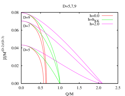
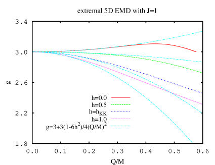
Figure 1: Left: Domain of existence of EMD black holes with equal-magnitude angular momenta in $D=5$, 7 and 9 dimensions. Right: Comparison of the gyromagnetic factor $g$ of $D=5$ extremal EMD black holes obtained with numerical and perturbative (cyan) methods.

The accuracy of the numerical method may be tested by means of the analytical KK solutions, as well as by exact relations (like the Smarr mass formula) these black holes satisfy [15].

As a complementary method one may employ perturbations to generate black hole solutions in higher dimensions [14, 15, 17]. The advantage of this method is that it produces analytical formulae, which the numerical method does not. However, the range of validity of these formulae is limited by the accuracy of the order of the perturbations.

A good perturbative parameter to produce charged rotating black hole solutions in higher dimensions is the electric charge. One starts from the MP solution [3] and expands the metric, the gauge potential and the dilaton in series expansions in the electric charge around the MP solution (see [15] for details). Those series are substituted in Eqs. (2-3) and solved order by order in the electric charge. For lower orders the equations are easy to solve but as the order of the perturbations increases the equations become more and more difficult to solve.

An important point when applying the perturbative method is the way the integration constants are fixed. One has to impose regularity of the solutions at the horizon together with the condition of asymptotic flatness. The Smarr mass formula is a useful means to check the accuracy of the solutions.

When the perturbative method is applied to extremal solutions the formulae simplify very much. For instance, one obtains the following formula of the gyromagnetic factor $g$ to second order

$$\frac{g}{D-2}=1+\frac{1}{4}\left[1-\frac{2(D-1)(D-2)}{(D-3)^{2}}h^{2}\right]\left(\frac{Q}{M}\right)^{2}+o\left(\left(\frac{Q}{M}\right)^{2}\right)\ ,$$ (8)

showing that the gyromagnetic factor is not constant for pure EM solutions ($h=0$).

4 Comparison of the two methods

Although both methods have a different range of applicability there is a region of the parameter space where both are valid, namely, when the electric charge is small. In that region one can check the consistency of the methods and their level of agreement [15]. This is presented in Figure 1 (right) where the perturbative formula Eq. (8) for extremal solutions is compared to the corresponding non-perturbative numerical results for $D=5$. We observe that for $|Q/M|\leq 0.2$ both approches are in good agreement. In fact, the perturbative method may be modified to analyze also slowly rotating solutions, using as the unperturbated initial solution the Tangherlini solution and using the angular momentum as the perturbative parameter.

To summarize, these two methods are complementary and provide us with a powerful tool to analyze black holes in higher dimensions when analytical solutions are not available.

References

References

- [1] M. Heusler 1996 Black Hole Uniqueness Theorems (Cambridge: Cambrigde University Press).
- [2] F. R. Tangherlini 1963 Nuovo Cimento 77 636.
- [3] R. C. Meyers, and M. J. Perry 1986 Ann. Phys. (N.Y.) 172 304.
- [4] J. C. Breckenridge, D. A. Lowe, R. C. Myers, A. W. Peet, A. Strominger and C. Vafa 1996 Phys. Lett. B 381 423.
- [5] M. Cvetic̆ and Donam Youm 1996 Nucl.Phys. B 476 118.
- [6] D. Klemm and W. A. Sabra (2001) Phys. Lett. B 503 147.
- [7] M. Cvetic̆, H. Lü and C. N. Pope 2004 Phys. Lett. B 598 273.
- [8] S. Dimopoulos and G. Landsberg 2001 Phys. Rev. Lett. 87 161602.
- [9] R. Emparan and H. S. Reall 2002 Phys. Rev. Lett. 88 101101.
- [10] P. M. Llatas 1997 Phys. Lett. B 397 63.
- [11] J. Kunz, D. Maison, F. Navarro-Lérida and J. Viebahn 2006 Phys. Lett. B 639 95.
- [12] J. Kunz, F. Navarro-Lérida and A. K. Petersen 2005 Phys. Lett. B 614 104.
- [13] J. Kunz, F. Navarro-Lérida and J. Viebahn 2006 Phys. Lett. B 639 362.
- [14] M. Allahverdizadeh, J. Kunz and F. Navarro-Lérida 2010 Phys. Rev. D 82 024030 .
- [15] M. Allahverdizadeh, J. Kunz and F. Navarro-Lérida 2010 Phys. Rev. D 82 064034.
- [16] B. Kleihaus, J. Kunz and F. Navarro-Lérida 2002 Phys. Rev. D 66 104001.
- [17] F. Navarro-Lérida 2010 Gen. Rel. Grav. 42 2891.