$N_{f}=2+1+1$ flavours of twisted mass quarks: cut-off effects at
tree-level of perturbation theory

Abstract

We present a calculation of cut-off effects at tree-level of perturbation theory for the K and D mesons using the twisted mass formulation of lattice QCD. The analytical calculations are performed in the time-momentum frame. The relative sizes of cut-off effects are compared for the pion, the kaon and the D meson masses. In addition, different realizations of maximal twist condition are considered and the corresponding cut-off effects are analyzed.

, ,

1 Introduction

Lattice calculations in QCD have shown significant advances in the last years [1, 2]. Simulations at the physical value of the pion mass are carried out nowadays, including up, down and strange quarks as dynamical degrees of freedom. A further step to render lattice QCD calculations even more realistic is also to include the charm quark in the simulations. In fact the simulations with two quark generations have already been started [3, 4, 5, 6, 7, 8]. Clearly, having the dynamical charm degree of freedom allows to test many physical aspects of the charm sector of QCD, such as the mesonic and baryonic spectrum and decay constants, heavy quark effects in operator matrix elements, the renormalized charm quark mass and eventually the running of the strong coupling constant for four flavours.

One concern when adding a charm quark mass is that lattice spacing effects may become large. Even in $\mathcal{O}(a)$-improved lattice theories cut-off effects of $\mathcal{O}(a^{2}m_{\mathrm{charm}}^{2})$ are expected to be present which then can become significant due to the rather large value of the charm quark mass. In this paper, we want to investigate Wilson twisted mass fermions [9, 10, 11] in a formulation that comprises mass degenerate light up and down quarks and mass non-degenerate strange and charm quarks, which we refer to as $N_{f}=2+1+1$ setup. All our calculations were performed at maximal twist, where automatic $\mathcal{O}(a)$-improvement is realized. The particular goal of this paper is to prepare the analytical basis for a study of the lattice spacing effects at tree-level of perturbation theory. To this end, following Refs. [12, 13, 14], we derive the quark propagators both for the 4-dimensional discrete momentum representation and the time-momentum representation in this $N_{f}=2+1+1$ setup. From the expressions of these propagators we construct the full (four times four) matrix of the correlation functions for K and D mesons.

Although calculations at tree-level of perturbation theory cannot be a quantitative measure for the interacting case when gluon degrees of freedom are incorporated, the qualitative results obtained in such setup can nevertheless serve as a valuable indicator. Studying the relative size of lattice spacing effects for the pion, the K and D mesons provides important information how cut-off effects behave when light and heavy quarks are considered.

In the twisted mass formulation of lattice QCD, the situation of maximal twist is of particular importance since in this case all physical observables are automatically $\mathcal{O}(a)$-improved. We don’t need an operator improvement and the calculation of corresponding coefficients. In the interacting case, maximal twist is realized by tuning of the Wilson quark mass to its critical value. As numerical and theoretical investigations in the past have demonstrated, see Refs. [15, 16, 17, 18, 19], there are, however, optimal and non-optimal ways to realize maximal twist.

At tree-level of perturbation theory, we study the analogs of these definitions of maximal twist. The optimal definition of maximal twist in the interacting case is to tune the PCAC quark mass to zero, which corresponds to setting the bare Wilson quark mass to zero at tree-level. The choice of tuning of the theory to maximal twist is not unique. Any definition of the critical quark mass that differs from the optimal one by $\mathcal{O}(a)$ effects still leads to maximal twist. However, such definitions can introduce unwanted, chirally enhanced $\mathcal{O}(a^{2})$ effects, i.e. terms that go like $\mathcal{O}(a^{2}/m_{\pi}^{2})$ and are hence called non-optimal. Our setup of tree-level of perturbation theory allows us to study both choices, the optimal tuning and the non-optimal tuning to maximal twist and we explore both options in this paper to understand better the behaviour of meson masses as functions of $a^{2}$, when different tuning conditions are employed.

2 Tree level of QCD with $N_{f}=2+1+1$ flavours of quarks

2.1 Tree level of QCD in the continuum

2.1.1 Physical basis versus twisted basis

We consider a light degenerate quark doublet $\psi^{(l)}=\{\psi^{(u)},\psi^{(d)}\}$ with a mass $m_{u,d}$ and a heavy non-degenerate quark doublet $\psi^{(h)}=\{\psi^{(c)},\psi^{(s)}\}$ with masses $m_{c}\neq m_{s}$. At tree-level of perturbation theory, i.e. in the absence of any gauge field, the light and heavy quark actions in the physical basis read:

$$S_{l}=\int d^{4}x\,\bar{\psi}^{(l)}(x)\Big{(}\gamma_{\mu}\partial_{\mu}+m_{u,d}\Big{)}\psi^{(l)}(x),\\$$ (1)

$$S_{h}=\int d^{4}x\,\bar{\psi}^{(h)}(x)\Big{(}\gamma_{\mu}\partial_{\mu}+\textrm{diag}(m_{c},m_{s})\Big{)}\psi^{(h)}(x).$$ (2)

Expressing the physical basis quark fields $\psi^{(l)}$ and $\psi^{(h)}$ in terms of twisted basis quark fields $\chi^{(l)}$ and $\chi^{(h)}$ via the twist rotation:

$$\psi^{(l)}=e^{i\omega_{l}\gamma_{5}\tau_{3}/2}\chi^{(l)},\ \ \ \psi^{(h)}=e^{i\omega_{h}\gamma_{5}\tau_{1}/2}\chi^{(h)}$$ (3)

yields:

$$S_{l}=\int d^{4}x\,\bar{\chi}^{(l)}(x)\Big{(}\gamma_{\mu}\partial_{\mu}+m_{0,l}+i\mu_{q}\gamma_{5}\tau_{3}\Big{)}\chi^{(l)}(x),$$ (4)

with: $m_{0,l}=m_{u,d}\cos(\omega_{l})$, $\mu_{q}=m_{u,d}\sin(\omega_{l})$ and

$$S_{h}=\int d^{4}x\,\bar{\chi}^{(h)}(x)\Big{(}\gamma_{\mu}\partial_{\mu}+m_{0,h}+i\mu_{\sigma}\gamma_{5}\tau_{1}+\mu_{\delta}\tau_{3}\Big{)}\chi^{(h)}(x),$$ (5)

where: $m_{0,h}=((m_{c}+m_{s})/2)\cos(\omega_{h})$, $\mu_{\sigma}=((m_{c}+m_{s})/2)\sin(\omega_{h})$ and $\mu_{\delta}=(m_{c}-m_{s})/2$ respectively (the Dirac matrices $\gamma_{\mu}$ [$\mu=0,1,2,3$] and $\gamma_{5}$ act in spinor space and the Pauli matrices $\tau_{a}$ [$a=1,2,3$] act in the flavour space), $\omega_{l}$ and $\omega_{h}$ are the so-called light and heavy twist angles.

The above relations between the quark masses and the mass parameters in the twisted basis quark actions can be solved with respect to the quark masses:

$$m_{u,d}=\sqrt{(m_{0,l})^{2}+(\mu_{q})^{2}},\\$$ (6)

$$m_{s}=\sqrt{(m_{0,h})^{2}+(\mu_{\sigma})^{2}}-\mu_{\delta},\ \ \ m_{c}=\sqrt{(m_{0,h})^{2}+(\mu_{\sigma})^{2}}+\mu_{\delta}.$$ (7)

At maximal twist $\omega_{l}=\omega_{h}=\pi/2$, corresponding to $m_{0,l}=m_{0,h}=0$, these relations simplify to:

$$m_{u,d}=\mu_{q},\ \ \ m_{s}=\mu_{\sigma}-\mu_{\delta},\ \ \ m_{c}=\mu_{\sigma}+\mu_{\delta}.$$ (8)

2.1.2 Meson spectrum

At tree-level of QCD, i.e. in absence of gluonic fields and, therefore, of any interactions between quarks, mesons correspond to free quark-antiquark pairs. For mesons at rest, i.e. with total momentum $\mathbf{P}=0$, the quark and the antiquark have to have opposite momenta $+\mathbf{p}$ and $-\mathbf{p}$. For example the spectra of K and D mesons are given by:

$$m_{K}(\mathbf{p})=\sqrt{(m_{s})^{2}+\mathbf{p}^{2}}+\sqrt{(m_{u,d})^{2}+\mathbf{p}^{2}},\ \ \ m_{D}(\mathbf{p})=\sqrt{(m_{c})^{2}+\mathbf{p}^{2}}+\sqrt{(m_{u,d})^{2}+\mathbf{p}^{2}}.$$ (9)

When we consider infinitely extended space, there is a continuum of states parametrized by momentum $\pm\mathbf{p}$ associated with the quark-antiquark pair. When considering a finite spatial volume $L^{3}$, only discrete momenta $\mathbf{p}=2\pi\mathbf{n}/L$, $\mathbf{n}\in\mathbb{Z}^{3}$ are possible, rendering the meson spectra also discrete. In both cases all states are two-fold degenerate, corresponding to parity $\mathcal{P}=-$ and $\mathcal{P}=+$. An exception are mesons with quark momentum $\mathbf{p}=0$, for which one can show that at tree-level they only exist for negative parity.

2.2 Tree level of perturbation theory of twisted mass lattice QCD

The lattice discretizations of the twisted basis quark actions (4) and (5) are: [9, 10]

$$S_{l}=a^{4}\sum_{x}\bar{\chi}^{(l)}(x)\Big{(}D_{\textrm{W}}(m_{0,l})+i\mu_{q}\gamma_{5}\tau_{3}\Big{)}\chi^{(l)}(x),\\$$ (10)

$$S_{h}=a^{4}\sum_{x}\bar{\chi}^{(h)}(x)\Big{(}D_{\textrm{W}}(m_{0,h})+i\mu_{\sigma}\gamma_{5}\tau_{1}+\mu_{\delta}\tau_{3}\Big{)}\chi^{(h)}(x),$$ (11)

where $D_{\mathrm{W}}$ denotes the standard Wilson Dirac operator:

$$D_{\mathrm{W}}(m_{0,x})=\frac{1}{2}\Big{(}\gamma_{\mu}\Big{(}\nabla_{\mu}+\nabla^{\ast}_{\mu}\Big{)}-a\nabla^{\ast}_{\mu}\nabla_{\mu}\Big{)}+m_{0,x},\ \ \ x\in\{l,h\}.$$ (12)

At maximal twist, physical observables are automatically $\mathcal{O}(a)$ improved, i.e. lattice discretization effects appear only quadratically [10, 11]. Although maximal twist can be realized in many different ways, there is an optimal definition of maximal twist corresponding to setting $m_{0,l}=m_{0,h}=0$ [16]. Note that for the light quark doublet, the Wilson term explicitly breaks isospin and parity, which becomes clear after a rotation to the physical basis. Only parity combined with light flavour exchange remains a symmetry. Since the Wilson term is $\mathcal{O}(a)$, isospin and parity are restored, when approaching the continuum limit. For the heavy quark doublet similar statements apply.

For infinite temporal extension, the lattice meson spectrum is expected to be qualitatively identical to the continuum meson spectrum discussed in Section 2.1.2. In particular, also on the lattice no positive parity mesons exist, with both quarks having zero momentum.

3 Twisted mass lattice quark propagators

The calculation of the heavy strange and charm quark propagators at tree-level of twisted mass lattice QCD is somewhat lengthy, but straightforward. Here we only quote the result, while details regarding the calculation can be found in App. A.

We can express the twisted mass action of the heavy doublet (11) in terms of the matrix $K(x;y)$:

$$S_{h}=a^{4}\sum_{x}\sum_{y}\bar{\chi}^{(h)}(x)K(x;y)\chi^{(h)}(y),$$ (13)

which is of the form:

$$K(x;y)=-\frac{1}{2a}\sum_{\mu=0}^{3}\Big{(}\delta_{x+\hat{\mu},y}(1-\gamma_{\mu})+\delta_{x-\hat{\mu},y}(1+\gamma_{\mu})\Big{)}+\delta_{x,y}\bigg{(}\Big{(}m_{0,h}+\frac{4}{a}\Big{)}+i\mu_{\sigma}\gamma_{5}\tau_{1}+\mu_{\delta}\tau_{3}\bigg{)},$$ (14)

where $x,y\in\mathbb{Z}$ denote space-time indices. The equation:

$$a^{4}\sum_{y}K(x;y)S^{(h)}(y;z)=\delta_{x,z}$$ (15)

relates $K(x;y)$ to the heavy twisted mass propagator $S^{(h)}(y;z)$ in position space representation.

In the time-momentum space representation, defined by:

$$\mathbf{S}^{(h)}(t,\mathbf{p})=\sum_{\mathbf{x}-\mathbf{y}}e^{-i\mathbf{p}(\mathbf{x}-\mathbf{y})}\mathbf{S}^{(h)}(x_{0},\mathbf{x};y_{0},\mathbf{y}),$$ (16)

where $t=x_{0}-y_{0}$, the resulting propagator for infinite temporal lattice extension reads:

$$\mathbf{S}^{(h)}(\mathbf{p},\pm|t|)=A_{(1)}\bigg{[}\Big{(}N_{(1)}-i\mu_{\sigma}\gamma_{5}\tau_{1}\Big{)}\Big{(}N_{(1)}^{2}+R_{(1)}^{2}-2\mu_{\delta}^{2}\Big{)}+\mu_{\delta}\tau_{3}\Big{(}R_{(1)}^{2}-N_{(1)}^{2}-2\mu_{\sigma}^{2}\Big{)}$$

$$-i\Big{(}N_{(1)}^{2}+R_{(1)}^{2}-2\mu_{\sigma}\mu_{\delta}\gamma_{5}\tau_{2}-2N_{(1)}\mu_{\delta}\tau_{3}\Big{)}\bigg{(}{\mathcal{K}}\pm\frac{i\gamma_{0}}{a}\sinh E_{(1)}\bigg{)}\bigg{]}+\Big{(}(1)\leftrightarrow(2)\Big{)},$$ (17)

with:

$$A_{(1),(2)}=-\frac{ae^{-E_{(1),(2)}|t|/a}}{4((M_{0,h}+1/a)^{2}-\mu_{\delta}^{2})\sinh E_{(1),(2)}(\cosh E_{(1),(2)}-\cosh E_{(2),(1)})},$$ (18)

$$N_{(1),(2)}=M_{0,h}+\frac{1}{a}\Big{(}1-\cosh E_{(1),(2)}\Big{)},\ \ \ R_{(1),(2)}^{2}={\mathcal{K}}^{2}+\mu_{\sigma}+\mu_{\delta}-\frac{1}{a^{2}}\sinh^{2}E_{(1),(2)},$$ (19)

$${\mathcal{K}}=\frac{1}{a}\sum^{3}_{j=1}\gamma_{j}\sin(p_{j}a),\ \ \ M_{0,x}=m_{0,x}+\frac{2}{a}\sum^{3}_{j=1}\sin^{2}(p_{j}a/2),\ \ \ x\in\{l,h\},$$ (20)

and the poles of the propagator in the energy-momentum space representation:

$$\cosh E_{(1),(2)}=\frac{-\tilde{b}\mp\sqrt{\tilde{b}^{2}-4\tilde{a}\tilde{c}}}{2\tilde{a}},$$ (21)

where:

$$\tilde{a}=\frac{4}{a^{2}}\bigg{(}\bigg{(}M_{0,h}+\frac{1}{a}\bigg{)}^{2}-\mu_{\delta}^{2}\bigg{)},$$ (22)

$$\tilde{b}=\frac{8}{a}\mu_{\delta}^{2}\bigg{(}M_{0,h}+\frac{1}{a}\bigg{)}-\frac{4}{a}s\bigg{(}M_{0,h}+\frac{1}{a}\bigg{)},$$ (23)

$$\tilde{c}=s^{2}-4\mu_{\sigma}^{2}\mu_{\delta}^{2}-4\mu_{\delta}^{2}\bigg{(}M_{0,h}+\frac{1}{a}\bigg{)}^{2},$$ (24)

$$s=\bigg{(}M_{0,h}+\frac{1}{a}\bigg{)}^{2}+\frac{1}{a^{2}}+{\mathcal{K}}^{2}+\mu_{\sigma}^{2}+\mu_{\delta}^{2}.$$ (25)

This analytical result for the heavy propagator has been checked by comparing with numerically computed propagators for various spatial lattice extensions and quark masses.

The corresponding light twisted mass propagator has been calculated in [13]. It reads:

$$\mathbf{S}^{(l)}(\mathbf{p},\pm|t|)=B\Big{(}\Big{(}1-\cosh E+aM_{0,l}\Big{)}\pm\gamma_{0}\sinh E-ia{\mathcal{K}}-ia\mu_{q}\gamma_{5}\tau_{3}\Big{)},$$ (26)

where ${\mathcal{K}}$ and $M_{0,l}$ are defined in (20) and

$$B=\frac{e^{-E|t|/a}}{2\sinh E(1+aM_{0,l})},\ \ \ \cosh E=\frac{(aM_{0,l}+1)^{2}+{\mathcal{K}}^{2}a^{2}+\mu_{q}^{2}a^{2}+1}{2(1+aM_{0,l})}.$$ (27)

4 Correlation matrices for K and D mesons

To study cut-off effects at tree-level of perturbation theory for $N_{f}=2+1+1$ quark flavours, we consider the spectrum of K and D mesons. As already discussed in Section 2.1.2, such mesons consist of the light up/down antiquark and either the heavy strange or the heavy charm quark. Since there is no gluonic field at tree-level, both quarks are free particles.

To create such mesons with well defined quantum numbers, we apply meson creation operators $\mathcal{O}_{(h,\Gamma)}$ to the vacuum state $|\Omega\rangle$. In the physical basis in continuum QCD, a possible choice of appropriate operators is given by:

$$\mathcal{O}_{(h,\Gamma)}(t)=\int d^{3}x\,\bar{\psi}^{(u)}(\mathbf{x},t)\Gamma\psi^{(h)}(\mathbf{x},t).$$ (28)

The heavy flavour index $h\in\{s,c\}$ determines whether the K meson or the D meson is created, the $4\times 4$ matrix $\Gamma\in\{\gamma_{5},1\}$ realizes the total angular momentum $J=0$ and either the negative parity $\mathcal{P}=-$ or the positive parity $\mathcal{P}=+$ and the integration over space $\int d^{3}x$ yields the total momentum $\mathbf{P}=0$, i.e. assures that the light and the heavy quark have opposite momenta $\pm\mathbf{p}$. In principle, one could also fix the individual quark momenta $\pm\mathbf{p}$ by including a second integration over space, but we prefer to consider not only the ground state, but also higher states, to have a situation, which is more like one of the interacting case, i.e. beyond tree-level, where one cannot get rid of excited states at the stage of operator construction, see Refs. [6, 7] for an investigation of meson mass determinations in the interacting case.

On the lattice using the twisted mass formalism an equivalent set of meson creation operators is given by:

$$\mathcal{O}_{(h,\Gamma)}(t)=\sum_{\mathbf{x}}\,\bar{\chi}^{(u)}(\mathbf{x},t)\Gamma\chi^{(h)}(\mathbf{x},t).$$ (29)

Note, however, that at finite lattice spacing, even after a rotation to the physical basis, parity and heavy flavour are only approximate quantum numbers, because of explicit twisted mass flavour and parity breaking. For a detailed discussion of these issues we refer to [6, 7]. To extract meson masses, we first calculate $4\times 4$ correlation matrices with the four operators (29):

$$C_{(h_{1},\Gamma_{1}),(h_{2},\Gamma_{2})}(t_{1}-t_{2})=\langle\Omega|\Big{(}\mathcal{O}_{(h_{1},\Gamma_{1})}(t_{1})\Big{)}^{\dagger}\mathcal{O}_{(h_{2},\Gamma_{2})}(t_{2})|\Omega\rangle.$$ (30)

Details of this calculation, which uses the propagators from the previous section, are presented in App. B. Then, we extract the masses of the K and D mesons, as explained in details in App. C and [6].

5 Numerical results

In this section, we will present some results for the continuum limit scaling of meson masses using maximally twisted mass fermions. In the investigation below, we will employ both the optimal and non-optimal definitions of maximal twist.

5.1 Setup and physical parameters

We consider a setup, which is reminiscent of QCD with $N_{f}=2+1+1$ flavours of quarks: there is the degenerate doublet of light fermions (masses $m_{u,d}$) and the non-degenerate doublet of significantly heavier fermions (masses $m_{s}\approx 22m_{u,d}$ and $m_{c}\approx 284m_{u,d}$), where the ratios of masses have been chosen as observed in the nature for the up/down, strange and charm quarks. However, in contrast to QCD, we consider the fermions (to which we will also refer as “quarks”) at tree-level, i.e. there are no interactions of any kind.

We consider a $3$-dimensional spatial volume of extension $N^{3}$ with periodic boundary conditions. Having fixed the ratios of quark masses, there are two dimensionful parameters remaining, $N$ and $m_{u,d}$. Their dimensionless product $Nm_{u,d}$ fully determines the physical situation. We choose $Nm_{u,d}=0.01$. Roughly speaking, this assures that even for our smallest lattices, the heavy charm quark mass $m_{c}$ in lattice units is smaller than $1$ (see below for more details).

5.2 Continuum limit and lattice parameters

For our lattice computations, the following set of parameters has to be chosen: the number of lattice sites $N$ in spatial direction (i.e. the spatial lattice volume is $N^{3}$), the twisted quark masses $\mu_{q}$, $\mu_{\sigma}$, $\mu_{\delta}$ (in units of $N=1/a$) and the untwisted quark masses $m_{0,l}$ and $m_{0,h}$ (in units of $N=1/a$).

At tree-level of perturbation theory, the continuum limit ($a\rightarrow 0$) and the infinite volume limit ($N\rightarrow\infty$) are equivalent. This means that the role of lattice spacing $a$ is played simply by the inverse of the number of lattice points $N$.

To recover in the continuum limit the setup described in the previous subsection, the lattice parameters have to be chosen in the following way, if the optimal definition of maximal twist is used:

• Untwisted quark masses:

  $$m_{0,l}=m_{0,h}=0.$$ (31)

• Twisted quark masses:

  $$N\mu_{q}=m_{u,d},\ \ \ N(\mu_{\sigma}-\mu_{\delta})=m_{s},\ \ \ N(\mu_{\sigma}+\mu_{\delta})=m_{c}.$$ (32)

When approaching the continuum limit, we set the twisted quark masses as specified in (32), i.e. we use this choice of twisted quark masses also at finite lattice spacing. The actual values of the strange and the charm quark mass for our numerical simulations are chosen such that they correspond to the ratios of central values of quark mass estimates published by the Particle Data Group [20] – $m_{s}/m_{u,d}=21.5901$ and $m_{c}/m_{u,d}=284.091$. This implies that since $N(\mu_{\sigma}+\mu_{\delta})=Nm_{c}\approx 0.01\times 284=2.84$, even for our smallest lattices, corresponding to $N=4$, the heaviest quark mass in lattice units (equal to $\mu_{\sigma}+\mu_{\delta}$) is smaller than $1$.

Regarding the untwisted quark masses, we study different ways of approaching the continuum limit. A particular and optimal choice is $m_{0,l}=m_{0,h}=0$. However, any other choice $Nm_{0,l}=\mathcal{O}(1/N)$ and $Nm_{0,h}=\mathcal{O}(1/N)$ also corresponds to maximal twist. Therefore, we also study the choices:

$$Nm_{0,l}=\frac{c_{l}}{N},\ \ \ Nm_{0,h}=\frac{c_{h}}{N},$$ (33)

with $c_{l}$ and $c_{h}$ arbitrary, but constant. Note, however, that in practice such choices should not be considered since –while still keeping the $\mathcal{O}(a)$-improvement of the theory– they might lead to the chirally enhanced cut-off effects, as discussed in Refs. [15, 16, 17, 18, 19].

5.3 Numerical study of the continuum limit

We study the continuum limit by performing computations with various lattice volumes, ranging from $N^{3}=4^{3}$ to $N^{3}=96^{3}$. In Figs. 1, 2 and 4 we investigate the continuum limit of $m_{K}$ and $m_{D}$ for different realizations of maximal twist, $c\equiv c_{l}=c_{h}\in\{0,0.04,0.06,0.08,0.1\}$ (Fig. 1), $c\equiv c_{l}=c_{h}\in\{0,1.0,1.5,2.5\}$ (Fig. 2) and $c_{l}=0,c_{h}=0.1$ or $c_{l}=0.1,c_{h}=0$ or $c_{l}=c_{h}=0.1$ (Fig. 4). The curves in the plots correspond to fits of quartic polynomials in $1/N^{2}$:

$$Nm_{\pi,K,D}=a_{0}+a_{1}\frac{1}{N^{2}}+a_{2}\left(\frac{1}{N^{2}}\right)^{2}+a_{3}\left(\frac{1}{N^{2}}\right)^{3}+a_{4}\left(\frac{1}{N^{2}}\right)^{4}.$$ (34)

In the former case, i.e. for relatively small values of the parameter $c$ and large lattices ($N=32$ to $N=96$), we observe a linear dependence in $1/N^{2}=a^{2}$ (i.e. the values of higher order coefficients $a_{n}$ ($n\geq 2$) in (34) are very small). This is, of course, expected, since Wilson twisted mass lattice fermions at maximal twist guarantee the absence of $\mathcal{O}(a)$ discretization effects.

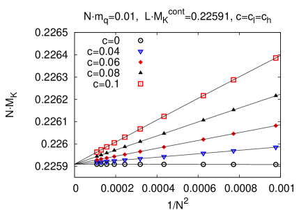
(a)

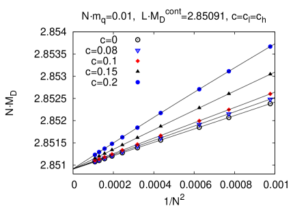
(b)

Figure 1: The cut-off effects and the continuum limit of: (a) kaon mass, (b) D meson mass, for different realizations of maximal twist $c\equiv c_{l}=c_{h}\in\{0,0.04,0.06,0.08,0.1\}$ and $32\leq N\leq 96$ lattices.

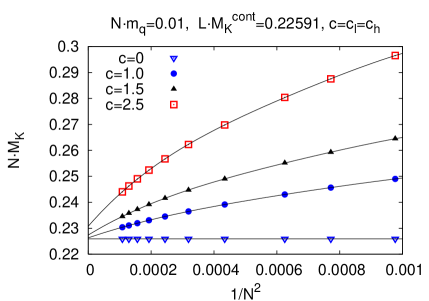
(a)

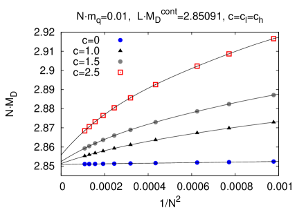
(b)

Figure 2: The cut-off effects and the continuum limit of: (a) kaon mass, (b) D meson mass, for different realizations of maximal twist $c\equiv c_{l}=c_{h}\in\{0,1.0,1.5,2.5\}$ and $32\leq N\leq 96$ lattices.

On the other hand, for large values of $c\equiv c_{l}=c_{h}$ (as shown in Fig. 2), both K and D meson masses as functions of $1/N^{2}$ clearly exhibit a non-vanishing curvature increasing with the value of $c$. However, this curvature can be well described by higher order corrections in $1/N^{2}$, as required from an $\mathcal{O}(a)$-improved theory. Nevertheless, when choosing the coefficients $c_{l,h}$ large, the theory is more and more tuned towards the Wilson quark action showing large cut-off effects. For very large $c$ values, also the extracted continuum limit values of meson masses are not reliable – because of the large curvature, in order to extrapolate to the continuum limit, one would need lattices with $N>96$ in such case. Of course, the values of $c_{l,h}$ used here are exceptionally large, leading to cases of non-optimal tuning to maximal twist that would never be used in practice. Hence, our investigation of these non-optimal tuning conditions serves solely illustrative purposes to indicate when higher order corrections in $1/N^{2}$ become relevant.

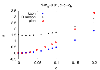
(a)

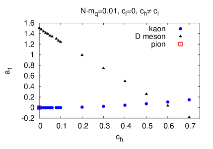
(b)

Figure 3: The slope $a_{1}$ in eq. (34) for the pion, kaon and D meson masses vs. the values of $c_{l}$ and $c_{h}$. (a) The case $c\equiv c_{l}=c_{h}$. (b) The case $c_{l}=0,\,c_{h}\geq 0$.

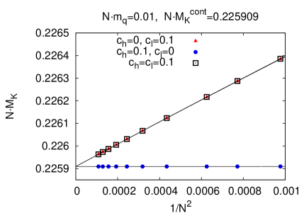
(a)

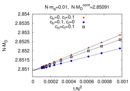
(b)

Figure 4: The cut-off effects and the continuum limit of: (a) kaon mass, (b) D meson mass, for different realizations of maximal twist: $(c_{l}=0,\,c_{h}\neq 0)$, $(c_{l}\neq 0,\,c_{h}=0)$, $(c_{l}=c_{h}\neq 0)$.

The values obtained for the $a_{0}$ coefficient correspond to meson masses extrapolated to the continuum limit. Within our numerical precision, they agree with the expected continuum results, i.e. the respective sums of the corresponding quark masses $Nm_{u,d}=0.010$, $Nm_{s}=0.21591$ and $Nm_{c}=2.84091$.

The slope parameter $a_{1}$ describes the magnitude of $\mathcal{O}(a^{2})$ discretization effects. The extracted values of this parameter are shown in Fig. 3 for the cases $c\equiv c_{l}=c_{h}$ and $c_{l}=0,\,c_{h}\geq 0$. In the case of $c_{l}=c_{h}=0$ (Fig. 3(a)), the cut-off effects are significantly larger for the D meson than for the K meson, while the smallest ones are observed for the pion. Considering the relative discretization effects, given by the ratios $a_{1}/a_{0}$, we observe that the cut-off effects are $\sim 10^{2}$ times larger for the D meson than for the K meson and $\sim 10^{3}$ times larger for the kaon than for the pion. Moreover, the size of discretization effects increases with increasing values of the parameter $c\equiv c_{l}=c_{h}$, but the sensitivity to this parameter is clearly the largest for the pion mass and it is very weak in the case of the D meson mass. This is an expected feature of the considered setup, since the non-vanishing bare Wilson quark mass, introduced by non-zero values of the parameter $c$, is relatively large in comparison with the pion mass and almost negligible as compared to the D meson mass (unless very large values of $c$ are considered). The case $c_{l}=0,\,c_{h}\geq 0$ (Fig. 3(b)) will be referred to below.

However, as we have already mentioned, $\mathcal{O}(a^{2}m_{q}^{2})$ effects are expected to be present in $\mathcal{O}(a)$-improved theories and they can become important in theories with heavy strange and charm quarks. Therefore, the $\mathcal{O}(a^{2})$ discretization effects given by the extracted parameter $a_{1}$ contain the “pure” $\mathcal{O}(a^{2})$ effects and in addition the $\mathcal{O}(a^{2}m_{q}^{2})$ effects.

In order to disentangle $\mathcal{O}(a^{2})$ and $\mathcal{O}(a^{2}m_{q}^{2})$ effects, we have computed the dependence of the K and D meson masses on $Nm_{s}$ and $Nm_{c}$, respectively, for fixed lattice size $N$. Then, we have fitted the following function to the lattice data:

$$NM_{\rm lat}-NM_{\rm cont}=b_{0}\frac{1}{N^{2}}+b_{1}\frac{(Nm_{q})^{2}}{N^{2}}+b_{2}\frac{(Nm_{q})^{4}}{N^{2}},$$ (35)

where: $NM_{\rm lat}$ – the lattice value of the K or D meson mass, $NM_{\rm cont}=Nm_{u,d}+Nm_{q}$ – its continuum ($N\rightarrow\infty$) counterpart, $q=s{\,\rm or\,}c$. The dependences of the K and D meson masses on $Nm_{q}$, together with the fit of the above functional form, are depicted in Fig. 5 for the case $c_{l}=c_{h}=0$. The extracted values of $b_{0},\,b_{1}$ and $b_{2}$ are shown in Table 1 for $c_{l}=c_{h}=0$, $c_{l}=c_{h}=0.1$ and $c_{l}=0,\,c_{h}=0.1$. For our fit, we have used $N=48$. However, we have checked for other lattice sizes ($N=16,\,32,\,64$) that the values of $b_{0},\,b_{1}$ and $b_{2}$ remain the same, within numerical precision.

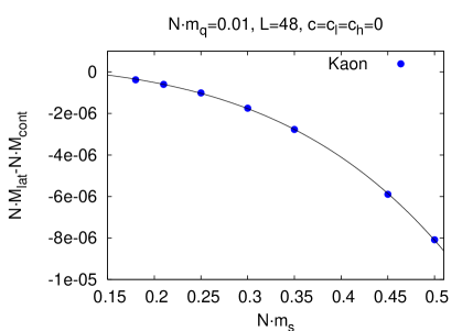
(a)

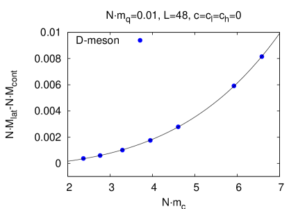
(b)

Figure 5: The $\mathcal{O}(a^{2})$, $\mathcal{O}(a^{2}m_{q}^{2})$ and $\mathcal{O}(a^{2}m_{q}^{4})$ effects (where $q=s,c$) in: (a) kaon mass, (b) D meson mass. The case of optimal tuning to maximal twist ($c_{l}=c_{h}=0$).

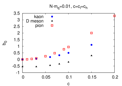
(a)

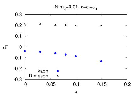
(b)

Figure 6: The extracted values of the parameters (a) $b_{0}$, (b) $b_{1}$, for different values of the parameter $c=c_{l}=c_{h}$. $b_{0}$ and $b_{1}$ are defined by eq. (35).

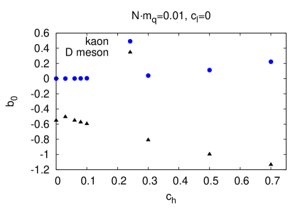
(a)

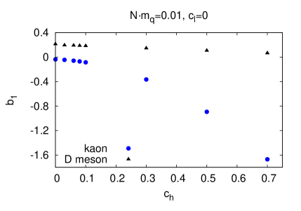
(b)

Figure 7: The extracted values of the parameters (a) $b_{0}$, (b) $b_{1}$, for different values of the parameter $c_{h}$, with $c_{l}=0$. $b_{0}$ and $b_{1}$ are defined by eq. (35).

	$c=c_{l}=c_{h}=0$		$c=c_{l}=c_{h}=0.1$		$c_{l}=0,\,c_{h}=0.1$
Coefficient	K meson	D meson	K meson	D meson	K meson	D meson
$b_{0}$	0.000571	-0.552	0.499	-0.199	0.00442	-0.596
$b_{1}$	-0.0373	0.214	-0.0848	0.198	-0.0848	0.183
$b_{2}$	-0.159	0.00540	-0.0623	0.00550	-0.0623	0.00592

Table 1: The fitting coefficients of eq. (35). The fits are shown in Fig. 5 for the case $N=48$, $c_{l}=c_{h}=0$.

	$c=c_{l}=c_{h}=0$		$c=c_{l}=c_{h}=0.1$		$c_{l}=0,\,c_{h}=0.1$
Effects	K meson	D meson	K meson	D meson	K meson	D meson
$\mathcal{O}(a^{2})$	$2.5\cdot 10^{-7}$	$-2.4\cdot 10^{-4}$	$2164\cdot 10^{-7}$	$-0.9\cdot 10^{-4}$	$19.2\cdot 10^{-7}$	$-2.6\cdot 10^{-4}$
$\mathcal{O}(a^{2}m_{q}^{2})$	$-7.6\cdot 10^{-7}$	$7.5\cdot 10^{-4}$	$-17\cdot 10^{-7}$	$6.9\cdot 10^{-4}$	$-17.2\cdot 10^{-7}$	$6.4\cdot 10^{-4}$
$\mathcal{O}(a^{2}m_{q}^{4})$	$-1.5\cdot 10^{-7}$	$1.5\cdot 10^{-4}$	$-0.6\cdot 10^{-7}$	$1.6\cdot 10^{-4}$	$-0.6\cdot 10^{-7}$	$1.7\cdot 10^{-4}$
sum	$-6.6\cdot 10^{-7}$	$6.6\cdot 10^{-4}$	$2146\cdot 10^{-7}$	$7.6\cdot 10^{-4}$	$1.4\cdot 10^{-7}$	$5.5\cdot 10^{-4}$

Table 2: The decomposition of the difference $NM_{\rm lat}-NM_{\rm cont}$ for the K and D mesons. The lattice size $N=48$, the strange quark mass $Nm_{s}=0.21591$ and the charm quark mass $Nm_{c}=2.84091$.

Our fits are summarized in Fig. 6 (for the case $c\equiv c_{l}=c_{h}$) and Fig. 7 (for $c_{l}=0,\,c_{h}\geq 0$). Fig. 6(a) shows the magnitude of “pure” $\mathcal{O}(a^{2})$ effects for the pion, the kaon and the D meson. In the region of small values of the parameter $c$, these effects are the largest for the D meson and comparable to each other for the pion and the kaon. Moreover, the curve $b_{0}(c)$ coincides with the curve $a_{1}(c)$ in Fig. 3(a), since in the case of the pion $\mathcal{O}(a^{2}m_{u,d}^{2})$ effects are negligible, due to the small value of light quark masses. We also observe that the value of $b_{0}$ increases with increasing $c$. However, since $b_{0}<0$ for the D meson in this region, the size of $\mathcal{O}(a^{2})$ effects decreases when the parameter $c$ increases, which means that the effects of non-optimal tuning can partially cancel $\mathcal{O}(a^{2})$ effects. For a particular value of the parameter $c$ (around 0.13) a complete cancellation can even occur (i.e $b_{0}=0$ can result).

Fig. 6(b) shows the magnitude of $\mathcal{O}(a^{2}m_{q}^{2})$ effects for the kaon and the D meson. These effects depend only slightly on the value of the parameter $c$. Interestingly, the sign of $\mathcal{O}(a^{2}m_{q}^{2})$ is opposite to the sign of the “pure” $\mathcal{O}(a^{2})$ effects, which means that a partial cancellation between these two types of effects occurs.

Further insight into the role of a method of tuning to maximal twist can be obtained by analyzing the dependence of cut-off effects for $c_{l}=0$ and $c_{h}\geq 0$, i.e. if the Wilson mass $m_{0,l}$ is precisely tuned to maximal twist, while the Wilson mass $m_{0,h}$ is non-optimally tuned (Fig. 7). In such case, the $\mathcal{O}(a^{2})$ effects are again much larger for the D meson than for the kaon. What is more, the magnitude of these effects is much smaller for the kaon than in the case $c_{l}=c_{h}$. This implies that non-optimal tuning in the light sector leads to much larger effects than non-optimal tuning in the heavy sector. Still, both effects tend to increase the value of the coefficient $b_{0}$. The situation is different for the D meson. There, the effects of non-optimal tuning of $m_{0,l}$ and $m_{0,h}$ have opposite signs and thus the “pure” $\mathcal{O}(a^{2})$ effects in the case $c_{l}=0,\,c_{h}>0$ increase with increasing value of the parameter $c_{h}$. In this way, the partial or complete cancellation of $\mathcal{O}(a^{2})$ effects that we have observed in the case $c_{l}=c_{h}$ can be attributed to non-optimal tuning of $m_{0,l}$ and not $m_{0,h}$.

Regarding the size of $\mathcal{O}(a^{2}m_{q}^{2})$ effects in the case $c_{l}=0,\,c_{h}\geq 0$, Fig. 7(b) shows that again non-optimal tuning in the light and in the heavy sector can have opposite effects. In the case of the D meson, a partial cancellation of $\mathcal{O}(a^{2}m_{q}^{2})$ effects can occur for positive values of the parameter $c_{h}$, but in the case of the kaon, the effects of non-optimal tuning of the Wilson mass $m_{0,h}$ reinforce the magnitude of $\mathcal{O}(a^{2}m_{q}^{2})$ effects.

It is also interesting to see the relative contribution of $\mathcal{O}(a^{2})$, $\mathcal{O}(a^{2}m_{q}^{2})$ and $\mathcal{O}(a^{2}m_{q}^{4})$ discretization effects to the difference $NM_{\rm lat}-NM_{\rm cont}$ for some chosen values of the lattice size and the strange and charm quark masses. Here we choose again $N=48$ and the quark masses considered in the earlier tests described in this section, i.e. $Nm_{s}=0.21591$, $Nm_{c}=2.84091$. The decomposition of the difference $NM_{\rm lat}-NM_{\rm cont}$ for such parameter values is shown in Table 2, for the cases $c_{l}=c_{h}=0$, $c_{l}=c_{h}=0.1$ and $c_{l}=0,\,c_{h}=0.1$.

The size of $\mathcal{O}(a^{2})$, $\mathcal{O}(a^{2}m_{q}^{2})$ and $\mathcal{O}(a^{2}m_{q}^{4})$ cut-off effects is of the same order of magnitude in the case of optimal tuning to maximal twist in both the light and the heavy sector. However, in this case the largest contribution to the difference $NM_{\rm lat}-NM_{\rm cont}$ is the one of $\mathcal{O}(a^{2}m_{q}^{2})$ effects, for both the K and D meson. Moreover, the relative sign of $\mathcal{O}(a^{2})$ and $\mathcal{O}(a^{2}m_{q}^{2})$ effects is different. The $\mathcal{O}(a^{2}m_{q}^{4})$ effects are roughly a factor of 5 smaller than $\mathcal{O}(a^{2}m_{q}^{2})$ effects in the case of both meson masses. Again, the overall size of discretization effects is much more important for the D meson than for the kaon, both if we consider absolute and relative cut-off effects.

In the case of non-optimal tuning of both $m_{0,l}$ and $m_{0,h}$, the $\mathcal{O}(a^{2})$ effects (induced by non-optimal tuning particularly in the light sector) are much more important than $\mathcal{O}(a^{2}m_{q}^{2})$ effects in the kaon case, but the latter still dominate in the case of the D meson.

An interesting situation occurs in the case $c_{l}=0,\,c_{h}=0.1$ for the kaon, where we observe that $\mathcal{O}(a^{2})$ effects are almost equal in magnitude, but of opposite sign to the $\mathcal{O}(a^{2}m_{q}^{2})$ effects. Thus, an almost exact cancellation occurs and the overall size of cut-off effects is much smaller than in the case of optimal tuning in both sectors. Such decrease of the overall size of discretization effects with respect to the optimal tuning case occurs also for the D meson, which is the effect that can be clearly observed in Fig. 3(b).

To summarize, we observe a very intricate interplay of different types of effects – $\mathcal{O}(a^{2})$, $\mathcal{O}(a^{2}m_{q}^{2})$ and even $\mathcal{O}(a^{2}m_{q}^{4})$ effects can become sizable. A partial or complete cancellation between $\mathcal{O}(a^{2})$ and $\mathcal{O}(a^{2}m_{q}^{2})$ effects is possible and moreover such cancellation can also occur between effects of non-optimal tuning to maximal twist in the light and heavy sectors. Needless to say, the behaviour in the interacting theory should be expected to be even more complex.

6 Conclusions

In this paper, we have provided an analytical basis for studying lattice spacing effects at tree-level of perturbation theory for maximally twisted mass Wilson quarks, when both the heavy quark doublet and the light one are included. Particularly, we have calculated the 4-dimensional momentum space and time-momentum frame quark propagators in the heavy sector and constructed the matrix of correlation functions for the K and D mesons.

We have investigated the scaling of the kaon and the D meson masses with the lattice spacing, for optimal and non-optimal tuning to maximal twist. We have clearly verified that the lattice spacing effects appear in even powers of $1/N=a$, as expected from the general automatic $\mathcal{O}(a)$-improvement of maximally twisted mass lattice QCD. More precisely, for the case of optimal tuning (given by the introduced parameter $c\equiv c_{l}=c_{h}=0$, where $c_{l}$ and $c_{h}$ determine the light and heavy Wilson mass: $Nm_{0,l}=c_{l}/N,\,Nm_{0,h}=c_{h}/N$) and non-optimal tuning with small $c$ values, we have observed the linear dependence of meson masses in $1/N^{2}=a^{2}$, while for sufficiently large $c$ values, the ${\mathcal{O}}(a^{4})$ and higher order corrections can become important.

We have also disentangled the $\mathcal{O}(a^{2})$, $\mathcal{O}(a^{2}m_{q}^{2})$ and $\mathcal{O}(a^{2}m_{q}^{4})$ discretization effects (where $m_{q}$ is the mass of the strange or the charm quark) in the kaon and the D meson masses and we have found a multitude of competing effects. The overall size of discretization effects can considerably depend on the details of tuning to maximal twist in both the light and the heavy sector. Partial cancellations (or even full cancellations for some particular values of parameters) can occur between the $\mathcal{O}(a^{2})$ effects and the $\mathcal{O}(a^{2}m_{q}^{2})$ effects and even between effects of non-optimal tuning in the light sector and the effects of non-optimal tuning in the heavy sector. Thus, non-optimal tuning can in certain instances decrease the overall size of discretization effects.

We believe that although our results do not provide any proofs for the interacting case, they give a clear warning: one should expect a very complex interplay of different effects and thus when physical observables in the strange and especially charm sectors are evaluated in full QCD, the enhanced cut-off effects should carefully be taken into account and physical results obtained at a single value of the lattice spacing can differ significantly from the continuum results.

Appendix A

The kernel of the heavy quark propagator:

$$K(x;y)=-\frac{1}{2a}\sum^{4}_{\mu=1}\left[(\delta_{\alpha\beta}-(\gamma_{\mu})_{\alpha\beta})\delta_{x+a\hat{\mu},y}+(\delta_{\alpha\beta}+(\gamma_{\mu})_{\alpha\beta})\delta_{x-a\hat{\mu},y}\right]\delta_{AB}\delta_{ij}+$$ (36)

$$\qquad\quad\;\,+\left[\left(m_{0,h}+\frac{4}{a}\right)\delta_{\alpha\beta}\delta_{ij}+i\mu_{\sigma}(\gamma_{5})_{\alpha\beta}\tau^{1}_{ij}+\mu_{\delta}\tau^{3}_{ij}\delta_{\alpha\beta}\right]\delta_{xy}\delta_{AB},$$

$$x=na,\ \ \ y=ma,\ \ \ n,m\in\mathbbm{Z}.$$

Further, we skip colour, flavour and Lorentz indices.

After discrete Fourier transformation:

$$K(p)=\sum_{x-y}K(x;y)e^{-ip(x-y)},$$ (37)

we get:

$$K(p)=\frac{i}{a}\sum^{4}_{i=1}\gamma_{i}\sin(p_{i}a)+\frac{1}{a}\left(1-\cos(p_{4}a)\right)+\frac{2}{a}\sum^{3}_{i=1}\sin^{2}\left(\frac{p_{i}a}{2}\right)+m_{0,h}+i\mu_{\sigma}\gamma_{5}\tau_{1}+\mu_{\delta}\tau_{3}.$$ (38)

Denote:

$$M_{0,h}=m_{0,h}+\frac{2}{a}\sum^{3}_{i=1}\sin^{2}\left(\frac{p_{i}a}{2}\right),\ \ \ N=M_{0,h}(p)+\frac{1}{a}(1-\cos(p_{4}a)),$$ (39)

$${\mathcal{K}}=\frac{1}{a}\sum^{3}_{i=1}\gamma_{i}\sin(p_{i}a),\ \ R^{2}=\mu_{\delta}^{2}+\mu_{\sigma}^{2}+{\mathcal{K}}^{2}+\frac{1}{a^{2}}\sin^{2}(p_{4}a).$$ (40)

Then, the matrix operator $K(p)$ takes the form:

$$K(p)=N+\mu_{\delta}\tau_{3}+i{\mathcal{K}}+i\mu_{\sigma}\gamma_{5}\tau_{1}.$$ (41)

The propagator can be calculated from the following relation:

$$S^{(h)}(p)K(p)=1,\ \ \ S^{(h)}(p)=\frac{K^{\dagger}(p)}{K(p)K^{\dagger}(p)}.$$ (42)

Using the properties of gamma matrices, we get the heavy twisted mass propagator:

$$S^{(h)}(p)=\frac{N+\mu_{\delta}\tau_{3}-i\sum^{4}_{\mu=1}\frac{\gamma_{\mu}}{a}\sin(p_{\mu}a)-i\mu_{\sigma}\gamma_{5}\tau_{1}}{N^{2}+R^{2}+2N\mu_{\delta}\tau_{3}+2\mu_{\sigma}\mu_{\delta}\gamma_{5}\tau_{2}}.$$ (43)

The denominator has the form $n+m\tau_{3}+l\tau_{2}$, where $n,m$ and $l$ are numbers. To eliminate the flavour structure from the denominator, we rearrange:

$$(n+m\tau_{3}+l\tau_{2})(n-m\tau_{3}-l\tau_{2})=(n+m\tau_{3})(n-m\tau_{3})+l\tau_{2}(n-m\tau_{3})-(n+m\tau_{3})l\tau_{2}-l^{2}=$$

$$n^{2}+mn\tau_{3}-nm\tau_{3}-m^{2}+ln\tau_{2}-lm\tau_{2}\tau_{3}-nl\tau_{2}-ml\tau_{3}\tau_{2}-l^{2}=n^{2}-m^{2}-l^{2}.$$ (44)

After this, we obtain:

$$S^{(h)}(p))=\frac{(N+\mu_{\delta}\tau_{3}-i\sum^{4}_{\mu=1}\frac{\gamma_{\mu}}{a}\sin(p_{\mu}a)-i\mu_{\sigma}\gamma_{5}\tau_{1})(N^{2}+R^{2}-2N\mu_{\delta}\tau_{3}-2\mu_{\sigma}\mu_{\delta}\gamma_{5}\tau_{2})}{(N^{2}+R^{2})^{2}-4N^{2}\mu_{\delta}^{2}-4\mu_{\sigma}^{2}\mu_{\delta}^{2}}.$$ (45)

The denominator of the last expression has two zeros which correspond to the poles of the propagator:

$$\cosh E_{1,2}=\cos(p_{4}a)_{1,2}=\frac{-b1\mp\sqrt{(b1)^{2}-4(a1)(c1)}}{2(a1)}.$$ (46)

We calculate the residues of the function:

$$f=\frac{ia}{8\pi}e^{-E\frac{t}{a}}\frac{L1(E)}{\left(\left(M_{0,h}+\frac{1}{a}\right)^{2}-\mu^{2}_{\delta}\right)(\cosh E-\cosh E_{1})(\cosh E-\cosh E_{2})}$$ (47)

The first residue is taken at the point $E=E_{1}$:

$${\bf{(res\ f)_{E=E_{1}}}}=\frac{ia}{8\pi}e^{-E_{1}\frac{t}{a}}\frac{P_{1}(E_{1})}{\left(\left(M_{0,h}+\frac{1}{a}\right)^{2}-\mu^{2}_{\delta}\right)\sinh E_{1}(\cosh E_{1}-\cosh E_{2})},$$ (48)

where:

$$P_{1}(E_{1})=N_{1}(N^{2}_{1}+R^{2}_{1}-2\mu^{2}_{\delta})+\mu_{\delta}(R^{2}_{1}-N_{1}^{2}-2\mu^{2}_{\sigma})\tau_{3}-i(N_{1}^{2}+R_{1}^{2})\left({\mathcal{K}}+\frac{i\gamma_{4}}{a}\sinh E_{1}\right)+$$

$$2i\mu_{\sigma}\mu_{\delta}\left({\mathcal{K}}+\frac{i\gamma_{4}}{a}\sinh E_{1}\right)\gamma_{5}\tau_{2}+2iN_{1}\mu_{\delta}\left({\mathcal{K}}+\frac{i\gamma_{4}}{a}\sinh E_{1}\right)\tau_{3}-i\mu_{\sigma}(N_{1}^{2}+R_{1}^{2}-2\mu^{2}_{\delta})\gamma_{5}\tau_{1},$$ (49)

$$N_{1}=M_{0,h}+\frac{1}{a}(1-\cosh E_{1}),\ \ \ \ \ R^{2}_{1}={\mathcal{K}}^{2}+\mu_{\sigma}+\mu_{\delta}-\frac{1}{a^{2}}\sinh^{2}E_{1}.$$ (50)

The second residue is at the point $E=E_{2}$:

$${\bf(res\ f)_{E=E_{2}}}=\frac{ia}{8\pi}e^{-E_{2}\frac{t}{a}}\frac{P_{1}(E_{2})}{\left(\left(M_{0,h}+\frac{1}{a}\right)^{2}-\mu^{2}_{\delta}\right)\sinh E_{2}(\cosh E_{2}-\cosh E_{1})},$$ (51)

where:

$$P_{1}(E_{2})=N_{2}(N^{2}_{2}+R^{2}_{2}-2\mu^{2}_{\delta})+\mu_{\delta}(R^{2}_{2}-N_{2}^{2}-2\mu^{2}_{\sigma})\tau_{3}-i(N_{2}^{2}+R_{2}^{2})\left({\mathcal{K}}+\frac{i\gamma_{4}}{a}\sinh E_{2}\right)+$$

$$2i\mu_{\sigma}\mu_{\delta}\left({\mathcal{K}}+\frac{i\gamma_{4}}{a}\sinh E_{2}\right)\gamma_{5}\tau_{2}+2iN_{2}\mu_{\delta}\left({\mathcal{K}}+\frac{i\gamma_{4}}{a}\sinh E_{2}\right)\tau_{3}-i\mu_{\sigma}(N_{2}^{2}+R_{2}^{2}-2\mu^{2}_{\delta})\gamma_{5}\tau_{1},$$ (52)

$$N_{2}=M_{0,h}+\frac{1}{a}(1-\cosh E_{2}),\ \ \ \ \ R^{2}_{2}={\mathcal{K}}^{2}+\mu_{\sigma}+\mu_{\delta}-\frac{1}{a^{2}}\sinh^{2}E_{2}.$$ (53)

The propagator is then the sum:

$${\bf S_{\infty}(\vec{p},t)}=2\pi i\left[(res\ f)_{E=E_{1}}+(res\ f)_{E=E_{2}}\right].$$ (54)

Appendix B

The elements of the correlation function matrix are calculated for infinite time using the expressions for infinite time twisted mass propagators (17) and (26). We show the calculation of one of them. We use the Fourier transformation, the definition of the $\delta$-function and gamma algebra:

$$C_{11}(t)=\sum_{\vec{x}}\langle(\bar{\psi}^{(u)}(x)\gamma_{5}\psi^{(s)}(x))^{\dagger}(\bar{\psi}^{(u)}(0)\gamma_{5}\psi^{(s)}(0)\rangle=$$

$$=\sum_{\vec{x}}{\rm Tr}\{\gamma_{5}S^{\bar{u}u}(\vec{x},t;0,0)\gamma_{5}S^{\bar{s}s}(0,0;\vec{x},t)\}=$$

$$=\sum_{\vec{x}}{\rm Tr}\left(\frac{1}{L^{3}}\sum_{\vec{p}}e^{i\vec{p}\vec{x}}S^{\bar{u}u}(\vec{p},t)\frac{1}{L^{3}}\sum_{\vec{q}}e^{-i\vec{q}\vec{x}}\gamma_{5}S^{\bar{s}s}(\vec{q},-t)\gamma_{5}\right)=$$ (55)

$$=\frac{1}{L^{3}}\sum_{\vec{p}}{\rm Tr}\left(\frac{1}{L^{3}}\sum_{\vec{q}}\sum_{\vec{x}}e^{i\vec{p}\vec{x}-i\vec{q}\vec{x}}S^{\bar{u}u}(\vec{p},t)\gamma_{5}S^{\bar{s}s}(\vec{q},-t)\gamma_{5}\right)=$$

$$=\frac{1}{L^{3}}\sum_{\vec{p}}{\rm Tr}\left(\frac{1}{L^{3}}\sum_{\vec{q}}\delta(\vec{p}-\vec{q})S^{\bar{u}u}(\vec{p},t)\gamma_{5}S^{\bar{s}s}(\vec{q},-t)\gamma_{5}\right)=$$

$$=\frac{1}{L^{3}}\sum_{\vec{p}}{\rm Tr}\left(S^{\bar{u}u}(\vec{p},t)\gamma_{5}S^{\bar{s}s}(\vec{p},-t)\gamma_{5}\right).$$

The components of the light and heavy quark propagators can be written in the following way:

$$S^{\bar{s}s}(\vec{p},-t)=\sum_{i=1}^{3}\gamma_{i}f_{i}+\gamma_{4}f_{4}+\mathbbm{1}\cdot f_{6},\ \ \ S^{\bar{u}u}(\vec{p},t)=\sum_{i=1}^{3}\gamma_{i}d_{i}+\gamma_{4}d_{4}+\gamma_{5}d_{5}+\mathbbm{1}\cdot d_{6}.$$ (56)

Thus, we get:

$${\rm Tr}\left\{S^{\bar{u}u}(\vec{p},t)\gamma_{5}S^{\bar{s}s}(\vec{p},-t)\gamma_{5}\right\}={\rm Tr}\Big{\{}\sum_{i=1}^{3}-d_{i}f_{i}-d_{4}f_{4}+d_{6}f_{6}\Big{\}}.$$ (57)

We identify the corresponding coefficients $f_{i}$ and $d_{i}$, where $i=1,..,6$ in the expressions (56) and (57) and obtain:

$$C_{11}(t)=\frac{N_{c}N_{d}}{L^{3}}\sum_{\vec{p}}\Big{\{}aC{\mathcal{K}}^{2}[A(N^{2}_{1}+R^{2}_{1})+B(N^{2}_{2}+R^{2}_{2})+2\mu_{\delta}(AN_{1}+BN_{2})]+$$ (58)

$$+\frac{C\sinh E_{1}^{l}}{a}\left[A(N_{1}^{2}+R_{1}^{2})\sinh E_{1}+B(N_{2}^{2}+R_{2}^{2})\sinh E_{2}+2\mu_{\delta}(AN_{1}\sinh E_{1}+BN_{2}\sinh E_{2})\right]+$$

$$+C(1-\cosh E_{1}^{l}+aM_{0,l})[AN_{1}(N_{1}^{2}+R_{1}^{2}-2\mu^{2}_{\delta})+BN_{2}(N_{2}^{2}+R_{2}^{2}-2\mu^{2}_{\delta})-$$

$$-\mu_{\delta}[A(R^{2}_{1}-N_{1}^{2}-2\mu^{2}_{\delta})+B(R^{2}_{2}-N^{2}_{2}-2\mu^{2}_{\sigma})]]\Big{\}}.$$

$$C_{22}(t)=\sum_{\vec{x}}\langle(\bar{\psi}^{(u)}(x)\gamma_{5}\psi^{(c)}(x))^{\dagger}\bar{\psi}^{(u)}(0)\gamma_{5}\psi^{(c)}(0)\rangle=$$

$$\frac{N_{c}N_{d}}{L^{3}}\sum_{\vec{p}}\Big{\{}aC{\mathcal{K}}^{2}[A(N^{2}_{1}+R^{2}_{1})+B(N^{2}_{2}+R^{2}_{2})-2\mu_{\delta}(AN_{1}+BN_{2})]+$$ (59)

$$+\frac{C\sinh E_{1}^{l}}{a}\left[A(N_{1}^{2}+R_{1}^{2})\sinh E_{1}+B(N_{2}^{2}+R_{2}^{2})\sinh E_{2}-2\mu_{\delta}(AN_{1}\sinh E_{1}+BN_{2}\sinh E_{2})\right]+$$

$$+C(1-\cosh E_{1}^{l}+aM_{0,l})[AN_{1}(N_{1}^{2}+R_{1}^{2}-2\mu^{2}_{\delta})+BN_{2}(N_{2}^{2}+R_{2}^{2}-2\mu^{2}_{\delta})+$$

$$+\mu_{\delta}[A(R^{2}_{1}-N_{1}^{2}-2\mu^{2}_{\delta})+B(R^{2}_{2}-N^{2}_{2}-2\mu^{2}_{\sigma})]]\Big{\}},$$

$$C_{33}(t)=\sum_{\vec{x}}\langle(\bar{\psi}^{(u)}(x)\psi^{(s)}(x))^{\dagger}\bar{\psi}^{(u)}(0)\psi^{(s)}(0)\rangle=$$

$$=\frac{N_{c}N_{d}}{L^{3}}\sum_{\vec{p}}\Big{\{}aC{\mathcal{K}}^{2}[A(N^{2}_{1}+R^{2}_{1})+B(N^{2}_{2}+R^{2}_{2})+2\mu_{\delta}(AN_{1}+BN_{2})]+$$ (60)

$$+\frac{C\sinh E_{1}^{l}}{a}\left[A(N_{1}^{2}+R_{1}^{2})\sinh E_{1}+B(N_{2}^{2}+R_{2}^{2})\sinh E_{2}+2\mu_{\delta}(AN_{1}\sinh E_{1}+BN_{2}\sinh E_{2})\right]-$$

$$-C(1-\cosh E_{1}^{l}+aM_{0,l})[AN_{1}(N_{1}^{2}+R_{1}^{2}-2\mu^{2}_{\delta})+BN_{2}(N_{2}^{2}+R_{2}^{2}-2\mu^{2}_{\delta})-$$

$$-\mu_{\delta}[A(R^{2}_{1}-N_{1}^{2}-2\mu^{2}_{\delta})+B(R^{2}_{2}-N^{2}_{2}-2\mu^{2}_{\sigma})]]\Big{\}},$$

$$C_{44}(t)=\sum_{\vec{x}}\langle(\bar{\psi}^{(u)}(x)\psi^{(c)}(x))^{\dagger}\bar{\psi}^{(u)}(0)\psi^{(c)}(0)\rangle=$$

$$=\frac{N_{c}N_{d}}{L^{3}}\sum_{\vec{p}}\Big{\{}aC{\mathcal{K}}^{2}[A(N^{2}_{1}+R^{2}_{1})+B(N^{2}_{2}+R^{2}_{2})-2\mu_{\delta}(AN_{1}+BN_{2})]+$$ (61)

$$+\frac{C\sinh E_{1}^{l}}{a}\left[A(N_{1}^{2}+R_{1}^{2})\sinh E_{1}+B(N_{2}^{2}+R_{2}^{2})\sinh E_{2}-2\mu_{\delta}(AN_{1}\sinh E_{1}+BN_{2}\sinh E_{2})\right]-$$

$$-C(1-\cosh E_{1}^{l}+aM_{0,l})[AN_{1}(N_{1}^{2}+R_{1}^{2}-2\mu^{2}_{\delta})+BN_{2}(N_{2}^{2}+R_{2}^{2}-2\mu^{2}_{\delta})+$$

$$+\mu_{\delta}[A(R^{2}_{1}-N_{1}^{2}-2\mu^{2}_{\delta})+B(R^{2}_{2}-N^{2}_{2}-2\mu^{2}_{\sigma})]]\Big{\}},$$

$$C_{43}(t)=\sum_{\vec{x}}\langle(\bar{\psi}^{(u)}(x)\psi^{(s)}(x))^{\dagger}\bar{\psi}^{(u)}(0)\psi^{(s)}(0)\rangle=$$

$$=\frac{N_{c}N_{d}}{L^{3}}\sum_{\vec{p}}aC\mu_{q}\mu_{\sigma}\{A(N_{1}^{2}+R^{2}_{1}-2\mu^{2}_{\delta})+B(N^{2}_{2}+R^{2}_{2}-2\mu^{2}_{\delta})\},$$ (62)

$$C_{34}(t)=\sum_{\vec{x}}\langle(\bar{\psi}^{(u)}(x)\psi^{(c)}(x))^{\dagger}\bar{\psi}^{(u)}(0)c(0)\rangle=$$

$$=\frac{N_{c}N_{d}}{L^{3}}\sum_{\vec{p}}aC\mu_{q}\mu_{\sigma}\{A(N_{1}^{2}+R^{2}_{1}-2\mu^{2}_{\delta})+B(N^{2}_{2}+R^{2}_{2}-2\mu^{2}_{\delta})\},$$ (63)

$$C_{31}(t)=\sum_{\vec{x}}\langle(\bar{\psi}^{(u)}(x)\psi^{(s)}(x))^{\dagger}\bar{\psi}^{(u)}(0)\gamma_{5}\psi^{(s)}(0)\rangle=$$

$$=\frac{N_{c}N_{d}}{L^{3}}\sum_{\vec{p}}(iaC\mu_{q})\{AN_{1}(N^{2}_{1}+R^{2}_{1}-2\mu^{2}_{\delta})+BN_{2}(N^{2}_{2}+R^{2}_{2}-2\mu^{2}_{\delta})-$$ (64)

$$-\mu_{\delta}[A(R^{2}_{1}-N^{2}_{1}-2\mu^{2}_{\sigma})+B(R^{2}_{2}-N^{2}_{2}-2\mu^{2}_{\sigma})]\},$$

$$C_{13}(t)=\sum_{\vec{x}}\langle(\bar{\psi}^{(u)}(x)\gamma_{5}\psi^{(s)}(x))^{\dagger}\bar{u}(0)\psi^{(s)}(0)\rangle=$$

$$=\frac{N_{c}N_{d}}{L^{3}}\sum_{\vec{p}}(-iaC\mu_{q})\{AN_{1}(N^{2}_{1}+R^{2}_{1}-2\mu^{2}_{\delta})+BN_{2}(N^{2}_{2}+R^{2}_{2}-2\mu^{2}_{\delta})-$$ (65)

$$-\mu_{\delta}[A(R^{2}_{1}-N^{2}_{1}-2\mu^{2}_{\sigma})+B(R^{2}_{2}-N^{2}_{2}-2\mu^{2}_{\sigma})]\},$$

$$C_{42}(t)=\sum_{\vec{x}}\langle(\bar{\psi}^{(u)}(x)\psi^{(c)}(x))^{\dagger}\bar{\psi}^{(u)}(0)\gamma_{5}\psi^{(c)}(0)\rangle=$$

$$=\frac{N_{c}N_{d}}{L^{3}}\sum_{\vec{p}}(iaC\mu_{q})\{AN_{1}(N^{2}_{1}+R^{2}_{1}-2\mu^{2}_{\delta})+BN_{2}(N^{2}_{2}+R^{2}_{2}-2\mu^{2}_{\delta})+$$ (66)

$$+\mu_{\delta}[A(R^{2}_{1}-N^{2}_{1}-2\mu^{2}_{\sigma})+B(R^{2}_{2}-N^{2}_{2}-2\mu^{2}_{\sigma})]\},$$

$$C_{24}(t)=\sum_{\vec{x}}\langle(\bar{\psi}^{(u)}(x)\gamma_{5}\psi^{(c)}(x))^{\dagger}\bar{\psi}^{(u)}(0)\psi^{(c)}(0)\rangle=$$

$$=\frac{N_{c}N_{d}}{L^{3}}\sum_{\vec{p}}(-iaC\mu_{q})\{AN_{1}(N^{2}_{1}+R^{2}_{1}-2\mu^{2}_{\delta})+BN_{2}(N^{2}_{2}+R^{2}_{2}-2\mu^{2}_{\delta})+$$ (67)

$$+\mu_{\delta}[A(R^{2}_{1}-N^{2}_{1}-2\mu^{2}_{\sigma})+B(R^{2}_{2}-N^{2}_{2}-2\mu^{2}_{\sigma})]\},$$

$$C_{12}(t)=\sum_{\vec{x}}\langle(\bar{\psi}^{(u)}(x)\gamma_{5}\psi^{(s)}(x))^{\dagger}\bar{\psi}^{(u)}(0)\gamma_{5}\psi^{(c)}(0)\rangle=$$

$$=\frac{N_{c}N_{d}}{L^{3}}\sum_{\vec{p}}(-aC\mu_{q}\mu_{\sigma})\left\{A(N^{2}_{1}+R^{2}_{1}-2\mu^{2}_{\delta})+B(N^{2}_{2}+R^{2}_{2}-2\mu^{2}_{\delta})\right\},$$ (68)

$$C_{21}(t)=\sum_{\vec{x}}\langle(\bar{\psi}^{(u)}(x)\gamma_{5}\psi^{(c)}(x))^{\dagger}\bar{\psi}^{(u)}(0)\gamma_{5}\psi^{(s)}(0)\rangle=$$

$$=\frac{N_{c}N_{d}}{L^{3}}\sum_{\vec{p}}(-aC\mu_{q}\mu_{\sigma})\left\{A(N^{2}_{1}+R^{2}_{1}-2\mu^{2}_{\delta})+B(N^{2}_{2}+R^{2}_{2}-2\mu^{2}_{\delta})\right\},$$ (69)

$$C_{14}(t)=\sum_{\vec{x}}\langle(\bar{\psi}^{(u)}(x)\gamma_{5}\psi^{(s)}(x))^{\dagger}\bar{\psi}^{(u)}(0)\psi^{(c)}(0)\rangle=$$

$$=\frac{N_{c}N_{d}}{L^{3}}\sum_{\vec{p}}\{-2iCa{\mathcal{K}}^{2}\mu_{\sigma}\mu_{\delta}(A+B)-\frac{2iC}{a}\sinh E_{1}^{l}\mu_{\sigma}\mu_{\delta}(A\sinh E_{1}+B\sinh E_{2})-$$ (70)

$$-iC\mu_{\sigma}(1-\cosh E_{1}^{l}+aM_{0,l})[A(N^{2}_{1}+R^{2}_{1}-2\mu^{2}_{\delta})+B(N^{2}_{2}+R^{2}_{2}-2\mu^{2}_{\delta})]\},$$

$$C_{41}(t)=\sum_{\vec{x}}\langle(\bar{\psi}^{(u)}(x)\psi^{(c)}(x))^{\dagger}\bar{\psi}^{(u)}(0)\gamma_{5}\psi^{(s)}(0)\rangle=$$

$$=\frac{N_{c}N_{d}}{L^{3}}\sum_{\vec{p}}\{2iCa{\mathcal{K}}^{2}\mu_{\sigma}\mu_{\delta}(A+B)+\frac{2iC}{a}\sinh E_{1}^{l}\mu_{\sigma}\mu_{\delta}(A\sinh E_{1}+B\sinh E_{2})+$$ (71)

$$+iC\mu_{\sigma}(1-\cosh E_{1}^{l}+aM_{0,l})[A(N^{2}_{1}+R^{2}_{1}-2\mu^{2}_{\delta})+B(N^{2}_{2}+R^{2}_{2}-2\mu^{2}_{\delta})]\},$$

$$C_{32}(t)=\sum_{\vec{x}}\langle(\bar{\psi}^{(u)}(x)\psi^{(s)}(x))^{\dagger}\bar{\psi}^{(u)}(0)\gamma_{5}\psi^{(c)}(0)\rangle=$$

$$=\frac{N_{c}N_{d}}{L^{3}}\sum_{\vec{p}}\{-2iCa{\mathcal{K}}^{2}\mu_{\sigma}\mu_{\delta}(A+B)-\frac{2iC}{a}\sinh E_{1}^{l}\mu_{\sigma}\mu_{\delta}(A\sinh E_{1}+B\sinh E_{2})+$$ (72)

$$+iC\mu_{\sigma}(1-\cosh E_{1}^{l}+aM_{0,l})[A(N^{2}_{1}+R^{2}_{1}-2\mu^{2}_{\delta})+B(N^{2}_{2}+R^{2}_{2}-2\mu^{2}_{\delta})]\}$$

$$C_{23}(t)=\sum_{\vec{x}}\langle(\bar{\psi}^{(u)}(x)\gamma_{5}\psi^{(c)}(x))^{\dagger}\bar{\psi}^{(u)}(0)\psi^{(s)}(0)\rangle=$$

$$=\frac{N_{c}N_{d}}{L^{3}}\sum_{\vec{p}}\{2iCa{\mathcal{K}}^{2}\mu_{\sigma}\mu_{\delta}(A+B)+\frac{2iC}{a}\sinh E_{1}^{l}\mu_{\sigma}\mu_{\delta}(A\sinh E_{1}+B\sinh E_{2})-$$ (73)

$$-iC\mu_{\sigma}(1-\cosh E_{1}^{l}+aM_{0,l})[A(N^{2}_{1}+R^{2}_{1}-2\mu^{2}_{\delta})+B(N^{2}_{2}+R^{2}_{2}-2\mu^{2}_{\delta})]\}.$$

Appendix C

From the $4\times 4$ correlation matrix in the twisted basis presented in App.B we get the masses of K and D mesons by solving a generalized eigenvalue problem [21]:

$$\sum_{k}C_{jk}(t){v}_{k}^{(n)}(t,t_{0})=\sum_{k}C_{jk}(t_{0}){v}_{k}^{(n)}(t,t_{0})\lambda^{(n)}(t,t_{0}),$$ (74)

where $k$ runs over $(h,\Gamma)$,  $h\in\{s,c\}$ and $\Gamma\in\{\gamma_{5},1\}$, $n=0,...,3$.

Eq. (74) leads to the following equation, giving the four effective masses $m^{(n)}_{\rm eff}$ for the lattice with temporal extension $T$:

$$\frac{\lambda^{(n)}(t,t_{0})}{\lambda^{(n)}(t+1,t_{0})}=\frac{e^{{-m^{(n)}_{\rm eff}}(t,t_{0})t}+e^{{-m^{(n)}_{\rm eff}}(t,t_{0})(T-t)}}{e^{{-m^{(n)}_{\rm eff}}(t,t_{0})(t+1)}+e^{{-m^{(n)}_{\rm eff}}(t,t_{0})(T-(t+1))}}.$$ (75)

Since we have performed the integration over $p_{4}$, our masses correspond to the limit of infinite $T$. We consider finite $t$ values, so the formula (75) becomes a ratio of two exponentials. For our tree level calculations, we have used $t_{0}\geqslant 10$. We have explored the dependence of the K and D masses on time and we have found that for the considered spatial extensions $L$ the mass plateaus are reached at $t\lesssim 100$.

We extract the meson masses from the plateaus at $t\in[50,120]$ (depending on the spatial extension $L$ of the lattices). In this range of $t$, our numerical precision gives plateaus of a very good quality and thus reliable data for the masses.

To determine the parity and flavour content of the four effective masses we perform the approximate rotation to pseudo physical basis [6]. After the rotation, the correlation matrix takes the form:

$$C^{\rm ph}_{(h,\Gamma)}(t)=M(\omega_{l},\omega_{h})C_{(h,\Gamma)}^{\chi}(t)M(\omega_{l},\omega_{h})^{\dagger}.$$ (76)

The twist rotation matrix is orthogonal at maximal twist and has the form:

$$M(\omega_{l},\omega_{h})=\left(\begin{matrix}\cos{\frac{\omega_{l}}{2}}\cos{\frac{\omega_{h}}{2}}&-\sin{\frac{\omega_{l}}{2}}\sin{\frac{\omega_{h}}{2}}&-i\sin{\frac{\omega_{l}}{2}}\cos{\frac{\omega_{h}}{2}}&-i\cos{\frac{\omega_{l}}{2}}\sin{\frac{\omega_{h}}{2}}\\ -\sin{\frac{\omega_{l}}{2}}\sin{\frac{\omega_{h}}{2}}&\cos{\frac{\omega_{l}}{2}}\cos{\frac{\omega_{h}}{2}}&-i\cos{\frac{\omega_{l}}{2}}\sin{\frac{\omega_{h}}{2}}&-i\sin{\frac{\omega_{l}}{2}}\cos{\frac{\omega_{h}}{2}}\\ -i\sin{\frac{\omega_{l}}{2}}\cos{\frac{\omega_{h}}{2}}&-i\cos{\frac{\omega_{l}}{2}}\sin{\frac{\omega_{h}}{2}}&\cos{\frac{\omega_{l}}{2}}\cos{\frac{\omega_{h}}{2}}&-\sin{\frac{\omega_{l}}{2}}\sin{\frac{\omega_{h}}{2}}\\ -i\cos{\frac{\omega_{l}}{2}}\sin{\frac{\omega_{h}}{2}}&-i\sin{\frac{\omega_{l}}{2}}\cos{\frac{\omega_{h}}{2}}&-\sin{\frac{\omega_{l}}{2}}\sin{\frac{\omega_{h}}{2}}&\cos{\frac{\omega_{l}}{2}}\cos{\frac{\omega_{h}}{2}}\end{matrix}\right)$$ (77)

and connects the operator ${\mathcal{O}}^{\rm ph}_{(h,\Gamma)}$ in pseudo physical basis with the ${\mathcal{O}}^{\chi}_{(h,\Gamma)}$ in the twisted mass one:

$${\mathcal{O}}^{\rm ph}_{(h,\Gamma)}=M(\omega_{l},\omega_{h}){\mathcal{O}}^{\chi}_{(h,\Gamma)},\ \ \ ({\mathcal{O}}^{\rm ph}_{(h,\Gamma)})^{\dagger}=({\mathcal{O}}^{\chi}_{(h,\Gamma)})^{\dagger}M^{T}(\omega_{l},\omega_{h}).$$ (78)

These bilinear operators are chosen in the following way:

$${\mathcal{O}}^{\rm ph}_{(h,\Gamma)}=\left(\begin{matrix}\bar{\psi}^{(u)}\gamma_{5}\psi^{s}\\ \bar{\psi}^{(u)}\gamma_{5}\psi^{c}\\ \bar{\psi}^{(u)}\psi^{s}\\ \bar{\psi}^{(u)}\psi^{c}\end{matrix}\right),\ \ \ \ \ \ \ \ {\mathcal{O}}^{\chi}_{(h,\Gamma)}=\left(\begin{matrix}\bar{\chi}^{(u)}\gamma_{5}\chi^{s}\\ \bar{\chi}^{(u)}\gamma_{5}\chi^{c}\\ \bar{\chi}^{(u)}\chi^{s}\\ \bar{\chi}^{(u)}\chi^{c}\end{matrix}\right).$$ (79)

References

- [1] K. Jansen, “Lattice QCD: a critical status report,” PoS LATTICE2008 (2008) 010 [arXiv:0810.5634 [hep-lat]].
- [2] E. E. Scholz, PoS LAT2009 (2009) 005 [arXiv:0911.2191 [hep-lat]].
- [3] T. Chiarappa et al., “Numerical simulation of QCD with u, d, s and c quarks in the twisted-mass Wilson formulation,” Eur. Phys. J. C 50, 373 (2007) [arXiv:hep-lat/0606011].
- [4] R. Baron et al., “First results of ETMC simulations with Nf=2+1+1 maximally twisted mass fermions,” PoS LAT2009 (2009) 104 [arXiv:0911.5244 [hep-lat]].
- [5] R. Baron et al., “Light hadrons from lattice QCD with light (u,d), strange and charm dynamical quarks,” JHEP 1006 (2010) 111 [arXiv:1004.5284 [hep-lat]].
- [6] R. Baron et al. [ETM Collaboration], “Computing and meson masses with twisted mass lattice QCD,” arXiv:1005.2042 [hep-lat].
- [7] R. Baron et al. [ETM Collaboration], “Kaon and meson masses with twisted mass lattice QCD,” arXiv:1009.2074 [hep-lat].
- [8] A. Bazavov et al. [MILC collaboration], Phys. Rev. D 82 (2010) 074501 [arXiv:1004.0342 [hep-lat]].
- [9] ALPHA Collaboration, R. Frezzotti, P. A. Grassi, S. Sint and P. Weisz, “Lattice QCD with a chirally twisted mass term,” JHEP 0108, 058 (2001) [arXiv:hep-lat/0101001].
- [10] R. Frezzotti and G. C. Rossi, “Twisted-mass lattice QCD with mass non-degenerate quarks,” Nucl. Phys. Proc. Suppl. 128 (2004) 193 [arXiv:hep-lat/0311008].
- [11] R. Frezzotti and G. C. Rossi, “Chirally improving Wilson fermions. I: improvement,” JHEP 0408, 007 (2004) [arXiv:hep-lat/0306014].
- [12] D. B. Carpenter and C. F. Baillie, “Free Fermion Propagators And Lattice Finite Size Effects,” Nucl. Phys. B 260 (1985) 103.
- [13] K. Cichy, J. Gonzalez Lopez, K. Jansen, A. Kujawa and A. Shindler, “Twisted mass, overlap and Creutz fermions: cut-off effects at tree-level of perturbation theory,” Nucl. Phys. B 800, 94 (2008) [arXiv:0802.3637 [hep-lat]].
- [14] K. Cichy, J. Gonzalez Lopez and A. Kujawa, “A comparison of the cut-off effects for Twisted Mass, Overlap and Creutz fermions at tree-level of Perturbation Theory,” Acta Phys. Polon. B 39 (2008) 3463 [arXiv:0811.0572 [hep-lat]].
- [15] K. Jansen, M. Papinutto, A. Shindler, C. Urbach and I. Wetzorke [XLF Collaboration], “Light quarks with twisted mass fermions,” Phys. Lett. B 619, 184 (2005) [arXiv:hep-lat/0503031].
- [16] R. Frezzotti, G. Martinelli, M. Papinutto and G. C. Rossi, “Reducing cutoff effects in maximally twisted lattice QCD close to the chiral limit,” JHEP 0604, 038 (2006) [arXiv:hep-lat/0503034].
- [17] S. R. Sharpe and J. M. S. Wu, “Twisted mass chiral perturbation theory at next-to-leading order,” Phys. Rev. D 71, 074501 (2005) [arXiv:hep-lat/0411021].
- [18] S. Aoki and O. Bar, “Automatic O(a) improvement for twisted-mass QCD in the presence of spontaneous symmetry breaking,” Phys. Rev. D 74, 034511 (2006) [arXiv:hep-lat/0604018].
- [19] K. Jansen, M. Papinutto, A. Shindler, C. Urbach and I. Wetzorke [XLF Collaboration], “Quenched scaling of Wilson twisted mass fermions,” JHEP 0509, 071 (2005) [arXiv:hep-lat/0507010].
- [20] C. Amsler et al. [Particle Data Group], Phys. Lett. B 667, 1 (2008) and 2009 partial update for the 2010 edition.
- [21] B. Blossier, M. Della Morte, G. von Hippel, T. Mendes and R. Sommer, “On the generalized eigenvalue method for energies and matrix elements in lattice field theory,” JHEP 0904, 094 (2009) [arXiv:0902.1265 [hep-lat]].