Prospects for sympathetic cooling of molecules
in electrostatic, ac and microwave traps

Abstract

We consider how trapped molecules can be sympathetically cooled by ultracold atoms. As a prototypical system, we study LiH molecules co-trapped with ultracold Li atoms. We calculate the elastic and inelastic collision cross sections of ⁷LiH + ⁷Li with the molecules initially in the ground state and in the first rotationally excited state. We then use these cross sections to simulate sympathetic cooling in a static electric trap, an ac electric trap, and a microwave trap. In the static trap we find that inelastic losses are too great for cooling to be feasible for this system. The ac and microwave traps confine ground-state molecules, and so inelastic losses are suppressed. However, collisions in the ac trap can take molecules from stable trajectories to unstable ones and so sympathetic cooling is accompanied by trap loss. In the microwave trap there are no such losses and sympathetic cooling should be possible.

I Introduction

There has been rapid progress in the field of cold and ultracold molecular gases over the last decade, driven by a diverse range of applications in physics and chemistry Carr09 . Polar molecules are of particular interest because they interact strongly with applied electric fields, and interact with one another through dipole-dipole interactions that are long-range, anisotropic, and tuneable. These properties, along with the exceptional control that is possible at low temperatures over all the degrees of freedom, make an ultracold gas of polar molecules an ideal tool for simulating strongly interacting condensed-matter systems and the remarkable quantum phenomena they exhibit Micheli06 . In low-temperature molecular gases it becomes possible to control chemical reactions using electric and magnetic fields and to study the role of quantum effects in determining chemical reactivity Krems:2005 . Cold molecules are also useful for testing fundamental symmetries, for example by measuring the value of the electron’s electric dipole moment Hudson et al. (2002), searching for a time-variation of fundamental constants Hudson et al. (2006); Bethlem et al. (2008); Bethlem and Ubachs (2009), or measuring parity violation in nuclei DeMille et al. (2008) or in chiral molecules Darquié et al. (2010). For these applications, a great leap in sensitivity could be obtained by cooling the relevant molecules to low temperatures so that, for example, the experiment could be done in a trap or a fountain Tarbutt et al. (2009b).

The bialkali molecules can be produced at very low temperatures by binding together ultracold alkali atoms, by either photoassociation Sage05 ; Deiglmayr08 or magnetoassociation Ospelkaus08 ; Lang08 ; Danzl08 ; Danzl10 . A few specific species of other molecules are amenable to direct laser cooling to ultralow temperatures Shuman10 . A large variety of useful molecules can be produced with temperatures in the range 10 mK to 1 K by decelerating supersonic beams Bethlem99 ; Narevicius08 ; Fulton06 or capturing the lowest-energy molecules formed in a cold buffer-gas source Weinstein98 ; vanBuuren09 . For many applications it is desirable to cool these molecules to lower temperatures, and this could be done by mixing the molecules with ultracold atoms and encouraging the two to thermalize. This sympathetic cooling method has not yet been demonstrated for neutral molecules, but is often used to cool neutral atoms Myatt97 ; Truscott01 ; Modugno01 , atomic ions Larson86 and molecular ions Drewsen04 ; Ostendorf97 .

For sympathetic cooling to yield ultracold molecules, the rate of atom-molecule elastic collisions, which are responsible for the cooling, must be sufficiently high that the molecules cool in the available time. In practice this requires that both atoms and molecules be trapped, so that they are held at high density and interact for a long time. The easiest way to trap molecules is in a static electric or magnetic trap. However, static traps can confine molecules only in weak-field-seeking states; since the ground state is always strong-field-seeking, inelastic collisions can eject molecules from the trap by de-exciting them to lower-lying strong-field-seeking states. These traps are therefore unsuitable for sympathetic cooling unless the ratio of the elastic to inelastic cross section happens to be particularly large. Inelastic losses can be avoided by trapping ground-state molecules, but such traps are more difficult to realize.

In this paper, we consider the sympathetic cooling of LiH molecules with ultracold Li atoms. Due to its large dipole moment of 5.88 D, its low mass, and its simple structure, LiH is an attractive molecule for studying the physics of dipolar gases and the electric field control of collisions and chemical reactions. A supersonic beam of cold LiH molecules has been produced Tokunaga07 and decelerated to low speed using a Stark decelerator Tokunaga09 . Ultracold Li is likely to be a good coolant for LiH because the closely matching masses ensures that energy is transferred efficiently in an elastic collision. Also, the low mass of Li ensures that inelastic collisions with non-zero angular momentum are suppressed by a centrifugal barrier, even at relatively high collision energies Lara06 . We have prepared a magneto-optical trap of $10^{10}$ Li atoms for the purpose of sympathetic cooling.

We begin by calculating the elastic and inelastic cross sections for LiH + Li collisions. Then we calculate the trajectories of a set of trapped LiH molecules that have occasional collisions with a co-trapped cloud of ultracold Li. Our aims are to calculate how the molecular temperature evolves with time, to investigate loss mechanisms in different kinds of traps, and to establish how the ultracold atoms should be distributed so that the cooling is most efficient.

II Scattering Calculations

We have carried out quantum-mechanical scattering calculations on ⁷Li+⁷LiH collisions on the potential energy surface of ref. Skomorowski et al., 2010. The calculations are carried out using the MOLSCAT program Hutson and Green (1994). We use full close-coupling calculations for the energy range of importance for sympathetic cooling, up to collision energies of 1 K, and coupled states (CS) calculations over an extended range up to 100 cm^-1. The calculations are carried out treating LiH as a rigid rotor, with rotational constant $b_{\rm LiH}/hc=7.5202$ cm^-1. Because of the deep potential well (8743 cm^-1) and strong anisotropy, a large rotational basis set is needed. The present calculations include all functions with LiH rotational quantum number $j$ up to $j_{\rm max}=37$. The coupled equations are solved using the hybrid log-derivative/Airy propagator of Alexander and Manolopoulos Alexander and Manolopoulos (1987) with the propagation continued to 500 Å.

The collision calculations treat the Li atom as structureless. This is justified because there are almost no terms in the collision Hamiltonian that can cause a change in the Li hyperfine state or magnetic projection quantum number Soldán et al. (2009); Żuchowski and Hutson (2009). The (very small) hyperfine structure of the LiH molecule is also neglected.

The results of close-coupling calculations for LiH molecules initially in $j=1$ are shown in Figure 1. As expected from the Wigner threshold laws Wigner (1948), the elastic cross section becomes constant at very low energy (below about 1 mK) and the inelastic cross section is approximately proportional to $E^{-1}$ in this region. Above about 10 mK the ratio of elastic to inelastic cross sections stabilizes at a factor of 5 to 10.

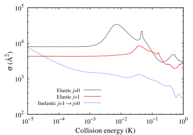
Figure 1: (color online) Elastic (red) and inelastic (blue) cross sections from close-coupling calculations on ⁷Li-⁷LiH with ⁷LiH initially in $j=1$. Also shown (black) are elastic cross sections for ⁷LiH initially in $j=0$.

Close-coupling calculations are carried out for fixed values of the total angular momentum $J$, and the resulting partial wave contributions are summed to form cross sections. The results in Figure 1 include contributions up to $J_{\rm max}=10$, and Figure 2 shows the individual partial wave contributions for $0<J\leq 6$. There is no significant resonance structure in the inelastic cross sections for $J<6$, although shape resonances appear in the elastic cross sections for $J\geq 2$ and are particularly prominent for $J=4$ and 6.

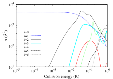
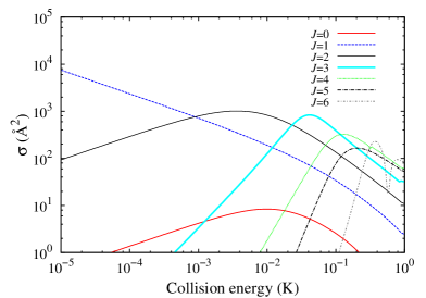
Figure 2: (color online) Partial-wave contributions to elastic (upper panel) and inelastic (lower panel) cross sections from close-coupling calculations.

The cross sections obtained from quantum scattering calculations on an individual potential energy surface are in general quite sensitive to small potential scalings because of variations in the scattering length $a$. However, this sensitivity is much smaller in Li+LiH because of the relatively low reduced mass. The low-energy limit of the elastic cross sections shown in Figure 1 may be compared with the value $\overline{\sigma}=4\pi\overline{a}^{2}=3200$ Å² obtained from the mean scattering length $\overline{a}=16.01$ Å, as defined by Gribakin and Flambaum Gribakin and Flambaum (1993).

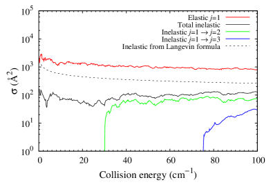
Figure 3: (color online) Elastic (red) and state-to-state inelastic cross sections from coupled states calculations on ⁷Li-⁷LiH with ⁷LiH initially in $j=1$. The dashed black line shows the Langevin limit for the total inelastic cross section.

The higher-energy results from CS calculations are shown in Fig. 3. It is interesting to compare the inelastic cross section with the Langevin limit, which assumes that all collisions that cross the centrifugal barrier lead to inelastic events. The Langevin limit is shown as a dashed line in Fig. 3, and it may be seen that the inelastic cross section remains below this limit even at collision energies around 100 cm^-1.

We note that the reaction $\text{LiH + Li}\rightarrow\text{Li}_{2}+\text{H}$ is highly endothermic and so cannot occur at the low collision energies of interest here.

III Sympathetic cooling simulations

Using the cross sections calculated in Section II, we simulate the sympathetic cooling of LiH molecules co-trapped with ultracold Li atoms. We consider three types of trap. The first is a static electric trap for molecules in the weak-field-seeking state $(j,m)=(1,0)$. Here, elastic collisions with the Li atoms cool the molecules, whereas an inelastic collision transfers a molecule to a lower-lying high-field-seeking state causing it to be lost from the trap. The other two traps we consider are a microwave trap and an ac electric trap, both of which can trap ground-state molecules so that inelastic losses are avoided. We note that sympathetic cooling in an optical dipole trap has been studied previously Barletta2010 .

III.1 Cooling in a static electric trap

We first consider the sympathetic cooling of LiH molecules in the weak-field-seeking $(j,m)=(1,0)$ state. The simulation starts with a large set of molecules with a velocity distribution that fills the trap. Later, when we consider ac and microwave traps, we will track individual molecular trajectories in these traps, but we do not need do this for the electrostatic trap. Our aim is only to calculate the fraction of all the molecules that cool to low temperature without being lost from the trap and this is determined entirely by the ratio of elastic to inelastic cross sections as a function of the collision energy.

For each collision we find the kinetic energy in the centre of mass frame, look up the relative probability for elastic and inelastic collisions as given in Figure 1, and then make a random choice between these two processes according to this probability. If the collision is inelastic, the molecule is lost from the trap. If the collision is elastic, the molecule’s velocity is transformed by the collision into a new velocity using a hard-sphere collision model. The velocity vector of the atom is selected at random from an isotropic Gaussian velocity distribution whose width is fixed by the temperature of the atom cloud, chosen here to be 140 $\mu$K. The atom and molecule velocities are transformed into the centre of momentum frame, where the molecular momenta before and after the collision, $\mathbf{p}$ and $\mathbf{p^{\prime}}$, are related by

$$\mathbf{p^{\prime}}=\mathbf{p}-2\left(\mathbf{p}\cdot\hat{\mathbf{e}}\right)\hat{\mathbf{e}},$$ (1)

where $\hat{\mathbf{e}}$ is a unit vector along the line joining the centres of the spheres. It is given by

$$\hat{\mathbf{e}}=\sqrt{1-|\mathbf{b}|^{2}}\frac{\mathbf{p}}{|\mathbf{p}|}+\mathbf{b}$$ (2)

where $\mathbf{b}$ is a vector that lies in the plane perpendicular to $\mathbf{p}$ and whose magnitude is the impact parameter of the collision normalized to the sum of the radii of the two spheres. For each collision, $\mathbf{b}$ is chosen at random from a uniform distribution subject to the constraints $\mathbf{b}\cdot\mathbf{p}=0$ and $|\mathbf{b}|\leq 1$. The new momentum of the molecule, $\mathbf{p^{\prime}}$, is finally transformed back into the lab frame and this momentum is used in the next collision.

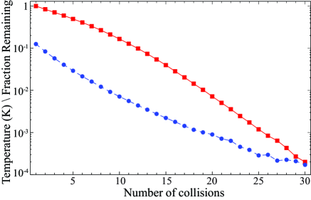
Figure 4: (Color online) Cooling and loss in a trap for weak-field-seeking molecules. The temperature of the molecules (blue circles) and the fraction remaining in the trap (red squares) are plotted against the number of collisions.

Figure 4 gives the results of these simulations, showing how the fraction of molecules remaining in the trap and the temperature of their distribution depends on the number of collisions that have occurred. The molecules have an initial temperature near 100 mK, and for every 10 collisions their temperature falls by about a factor of 10. After about 20 collisions, they have reached a temperature of 1 mK, but only 0.7% of them remain. After 28 collisions, the molecules have thermalized to the temperature of the atoms, but now the fraction that remains is only $4\times 10^{-4}$. We see that the ratio of elastic to inelastic cross sections is too small in this case for sympathetic cooling in a static trap to be feasible.

Our simulations use collision cross sections calculated in zero field, even though the molecules are electrostatically trapped. An electric field can have a large effect on atom-molecule collisions, as recently demonstrated for collisions between Rb and ND₃ in an electrostatic trap Parazzoli11 . Here, it was found that the trapping field increases the inelastic cross section. If a similar effect occurred for Li-LiH, it would strengthen our conclusion that sympathetic cooling is not feasible in the static trap for this system.

III.2 Cooling in an ac electric trap

To eliminate trap loss due to inelastic collisions, it is desirable to trap the molecules in their ground state. The ground state of every molecule is strong-field-seeking, and strong-field-seeking molecules cannot be trapped using static fields. One solution is to use an ac electric trap where the molecules move on a saddle-shaped potential that focusses them towards the centre of the trap in one direction, but defocusses them in another direction. By alternating the focussing and defocussing directions at a suitable rate, molecules are confined near the trap centre. Such ac electric traps have already been used to trap polar molecules in strong-field-seeking states vanVeldhoven05 ; Bethlem06 ; Schnell07 , and also to trap ground-state atoms Schlunk07 ; Rieger07 , and sympathetic cooling of molecules in ac traps has been proposed Schlunk07 ; Rieger07 .

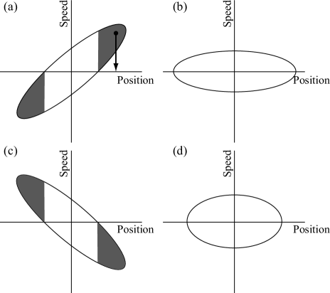
Figure 5: Phase-space acceptance of an ac trap in one dimension for 4 phases of the switching cycle: (a) start of focussing period, (b) centre of focussing period, (c) start of defocussing period, (d) centre of defocussing period. The shaded areas indicate regions of phase space that are unstable in an idealised head-on collision.

Motion in an ac trap consists of a small-amplitude micromotion at the switching frequency of the trap, superimposed on a larger-amplitude, lower-frequency macromotion. The stability of the molecules derives from the micromotion, and a collision which interrupts the micromotion may put the molecule onto an unstable trajectory. This means that a molecule initially confined in the trap may be ejected by a collision even though the collision reduces its energy. Figure 5 gives a simple picture of how this can happen. In each dimension, the set of all the stable molecules forms an ellipse in phase space, and this ellipse evolves periodically with the phase of the switching cycle Bethlem06 . Figure 5(a) shows the ellipse at the start of a focussing phase, showing that the positions and speeds of the molecules are positively correlated at this phase. To illustrate what may happen in a collision, consider the case where molecules collide head-on ($\mathbf{b}=0$) with stationary atoms of the same mass. In this idealised case, a collision reduces the speed of a molecule to zero, leaving its position unchanged, as indicated by the arrow in Figure 5(a). The molecule will remain trapped only if it is still inside the ellipse, so the shaded regions of the ellipse are unstable against collisions. The same arguments apply at the start of the defocussing phase, as indicated in Figure 5(c). Half-way through the focussing and defocussing phases (Figure 5(b,d)), the molecules remain inside the stable region when their speeds are reduced to zero and so there will be no collisional loss at these phases. The phase-space plots show what happens in only one dimension. In a cylindrically symmetric ac trap, the same plots can be made for the radial and longitudinal directions separately, one being half a period out of phase with the other. Thus when the focussing phase begins in the radial direction, the defocussing phase is beginning in the longitudinal direction, and a molecule must not be inside any of the shaded regions if it is to remain trapped after a collision.

This picture is, of course, a highly simplified one. The collisions do not reduce the speed to zero, and they can couple energy from one direction to another, which tends to increase the opportunities for loss. Nevertheless, we expect the same general conclusions to hold – a large portion of the trap’s stable phase-space volume becomes unstable when sympathetic cooling collisions are introduced, and collisions are more likely to result in loss at the start of a focus/defocus phase than half-way through.

Turning now to a complete simulation, we consider LiH molecules in a cylindrical ac trap consisting of two ring electrodes and two cylindrically symmetric end caps, as used in refs. vanVeldhoven05 ; Bethlem06 . The square of the electric field magnitude in this trap is well approximated by the expression

$$E^{2}(z,\rho)=E_{0}^{2}\left(1+2a_{3}\frac{(z^{2}-\frac{1}{2}\rho^{2})}{z_{0}^{2}}+a_{3}^{2}\frac{(z^{4}+\frac{1}{4}\rho^{4})}{z_{0}^{4}}\right.$$

$$\left.+2a_{5}\frac{(z^{4}-3z^{2}\rho^{2}+\frac{3}{8}\rho^{4})}{z_{0}^{4}}\right),$$ (3)

where $z_{0}$ is the characteristic size of the trap, $E_{0}$ is the electric field magnitude at the trap centre, and $a_{3}$ and $a_{5}$ are the coefficients in a multipole expansion of the electrostatic potential. Considering the same trap as used in ref. Bethlem06 , we set $a_{3}=-1.29$ and $a_{5}=0.63$ for the longitudinal focussing phase, $a_{3}=1.29$ and $a_{5}=0.44$ for the radial focussing phase, $z_{0}=4.55$ mm, and $E_{0}=50$ kV/cm. We switch the trap between the two configurations at a frequency of 5 kHz with a 50:50 duty cycle.

An ensemble of initially warm molecules evolves within the trap, each molecule having occasional collisions with a distribution of $10^{10}$ ultracold Li atoms. We calculate the trajectories of many molecules moving in the trap by solving the equations of motion numerically using a Runge-Kutta method with a fixed time step. The force acting on the molecules is $\mathbf{F}=-\mathbf{\nabla}W$ where $W$ is the Stark shift. For the electric field magnitudes considered here, the Stark shift of ground-state LiH is small compared to the rotational spacing, and is given to a good approximation by second-order perturbation theory:

$$W=-\frac{\mu_{e}^{2}E^{2}}{6b_{\rm LiH}}.$$ (4)

Here, $\mu_{e}$ is the electric dipole moment of the molecule and $b_{\rm LiH}$ is the rotational constant (in energy units).

We suppose that the atoms are trapped independently from the molecules, for example in a magnetic trap, and we give them a spherically symmetric Gaussian spatial distribution with a $1/e$ half-width $w_{a}=3$ mm, and a Maxwell-Boltzmann velocity distribution with a temperature $T_{a}=50\,\mu$K.

We first simulate trajectories without any collisions, starting with an initial phase-space distribution that is larger than the trap acceptance, so as to obtain a set of molecules that, in the absence of collisions, survive in the trap for 10 s. This set of molecules defines the phase-space acceptance of the trap and is then used for the full simulation including the collisions. This ensures that molecules are lost from the trap only as a result of collisions. After each interval of time $\Delta t$, the calculation of the molecular trajectory is stopped and the probability, $P$, of the molecule having a collision during this time interval is calculated. The value of $\Delta t$ is chosen such that $P\ll 1$ and we take $P=n\,\sigma(K)\,v\,\Delta t$, where $n$ is the local density of atoms, $v$ is the relative velocity of the LiH molecule and Li atom at the time of collision, and $\sigma(K)$ is the elastic collision cross section at collision energy $K$. A random number, $r$, is chosen from a uniform distribution in the interval from 0 to 1, and a collision occurs only if $P>r$. When a collision does occur, the velocity vector obtained from the molecular trajectory is transformed using the hard-sphere collision model outlined above. The numerical integration of the trajectory then continues using this transformed velocity. Since the number of trapped atoms is many orders of magnitude larger than the number of trapped molecules, we assume that the atom distribution is unaffected by the presence of the molecules. We also neglect collisions between the molecules, since their density is so low.

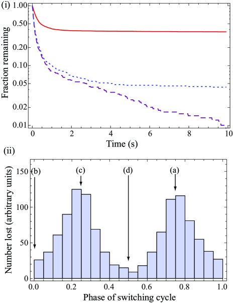
Figure 6: (Color online) Simulated molecule loss in an ac trap. (i) Fraction of molecules surviving as a function of time. Dashed (purple) line: real trap, $T_{a}=50\,\mu$K. Dotted (blue) line: real trap, $T_{a}=0$. Solid (red) line: ideal trap, $T_{a}=50\,\mu$K. (ii) Number of collisions that result in molecule loss as a function of the phase of the switching cycle, in an ideal trap. The zero of phase corresponds to the centre of the radial focussing period and the labels (a-d) refer to the phases depicted by the same labels in Figure 5.

The dashed line in Figure 6(i) shows the fraction of molecules that survive in the ac trap as a function of time. We see that most of the molecules are lost due to collisions and that this loss occurs on two separate time scales. During the first 1 s, 94% of all the molecules are lost from the trap. Between 1 s and 10 s the number of trapped molecules continues to fall, so that after 10 s only 1% remain in the trap. It is surprising to find that the loss continues at long times since we would expect there to be a small region close to the origin of phase space that is stable against collisions. It appears that even these molecules are eventually being destabilized by the collisions. To investigate why this happens, we repeated the simulation with the atom temperature reduced to zero. The result is shown by the dotted line in Fig. 6(i). Here, the loss at early times is the same as before, but after a few seconds of cooling the fraction remaining in the trap stabilizes at around 5%. When the atoms have non-zero temperature, the collisions cause molecules near the origin of phase-space to diffuse away from the origin, eventually ending up on an unstable trajectory. The atoms cool the hotter molecules, but they also tend to heat the coolest ones, and even when the atom temperature is only $50\,\mu$K the heating results in significant additional losses from the trap on a 10 s timescale.

Next, to shed some light on why there is so much collisional loss in the ac trap, we simplified the simulations by neglecting terms in the electric field beyond the second term in Eq. (III.2). In this harmonic approximation the phase-space acceptance of the trap is maximized, and although this field cannot be realized in practice Bethlem06 it is helpful to make this approximation since the dynamics in such an ideal ac trap are well understood. The higher-order terms complicate the dynamics by introducing nonlinear forces into the trap and coupling the axial and radial motions, and this greatly reduces the trap acceptance. Our simulations show that neglect of these higher-order terms increases the acceptance by a factor of 4 in both position and velocity. The solid line in Figure 6(i) shows the fraction of molecules that survive in the ideal ac trap as a function of time. In this case almost all the loss occurs in the first 1 s of cooling. The loss occurs from the outer regions of the trap and there is a ‘safe’ region around the phase-space origin where a molecule will remain inside the trap’s acceptance for all possible outcomes of a single collision. Once molecules have been cooled into this region there are no losses. The fraction of all the initial molecules that remain in the trap after 3 s is 38%, and there are no further losses between 3 s and 10 s. These results conform to the intuitive expectations obtained from our discussion of Figure 5. Comparing the results obtained for the ideal trap with those of the real trap, we see that it is primarily the large non-linear forces that make the ac trap an unsuitable environment for sympathetic cooling.

Figure 6(ii) shows how the number of collisions resulting in trap loss depends on the phase of the switching cycle, in the ideal ac trap. As expected from the discussion of Figure 5, the simulations confirm that collisions occurring at the start of a focussing / defocussing period are far more likely to cause loss than those occurring half-way through these periods. Similar results are obtained when the higher-order terms are included, except that the modulation observed in the figure is then not so deep.

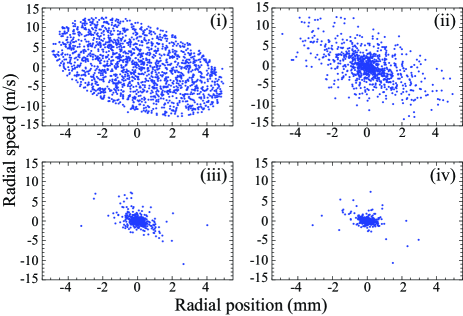
Figure 7: (Color online) Simulated time evolution of the radial phase-space distributions of molecules in an ideal ac trap overlapped with a 50 $\mu$K atom cloud with a width parameter of $w_{a}=3$ mm. Only the 1st and 2nd terms in Eq. (III.2) are included in the expression for the electric field. The phase of the switching cycle is the same in each plot and, to within one switching cycle, the times are (i) 0.002 s, (ii) 0.5 s, (iii) 3 s and (iv) 10 s.

Figure 7 shows how the radial phase-space distribution in the ideal ac trap evolves with time. At early times the molecules fill the available trap acceptance, but as time goes on they congregate near the origin of phase space. After 0.5 s [Figure 7(ii)] the ellipse has become dense near the centre and sparse elsewhere. Most molecules have had one or more collisions by this time and these collisions tend to remove molecules from the outer regions of the distribution, either by cooling them towards the centre or, as discussed above, kicking them out of the trap. As time goes on, almost all the molecules in the outer regions of phase space disappear and the molecules that remain are cooled into a small region near the origin. After 10 s [Figure 7(iv)] this cold distribution has a full width at half maximum of 0.3 mm in radial position and 0.9 m/s in radial speed. The time evolution of the longitudinal phase-space distribution is similar.

III.3 Cooling in a microwave trap

An alternative way to trap ground-state molecules is to use a microwave trap, as discussed in ref. DeMille04 . The ground-state molecules are attracted to the electric field maximum of the standing-wave microwave field inside a resonant cavity. The trap depth is particularly large when the detuning of the microwave frequency from the rotational transition frequency is small, although this places a stringent requirement that the microwave field be circularly polarised in order to avoid multi-photon excitation to rotationally excited states DeMille04 . Collision-induced absorption of microwave photons may also occur in the trap, and again this unwanted process is far more probable when the detuning is small Alyabyshev09 . Here, we consider a far-detuned microwave trap for ground-state LiH molecules, operating at a frequency of 15 GHz. Since this frequency is very small compared to the rotational frequency ($2b_{\rm LiH}/h=445$ GHz), and since the Stark shift will also be small compared to $b_{\rm LiH}$ for all attainable electric field strengths, the Stark shift is given to a good approximation by Eq. (4), where $E^{2}$ is now the time-averaged squared electric field. We take the microwave field to be the fundamental Gaussian mode of a symmetrical Fabry-Perot cavity, having a beam waist of 15 mm and an rms electric field at the trap centre of $E_{0}=40$ kV/cm. This is the field produced by coupling 2.6 kW of power into a cavity whose Q-factor is set by the reflectivity of room-temperature copper mirrors. The trap has a depth of 500 mK and the simulation begins with a trap whose phase-space acceptance is completely filled. We simulate individual molecular trajectories in the microwave trap with collisions modelled in exactly the same way as outlined above for the ac trap. We use the field-free elastic cross section shown in Fig. 1 since this is insensitive to the microwave field Alyabyshev09 , and we neglect inelastic relaxation between field-dressed states because, for our trap conditions, the rate of this inelastic process is expected to be very low compared to the elastic collision rate Alyabyshev09 .

Each time a molecule has a collision with an ultracold atom, its energy is reduced. Nevertheless, it is possible for a collision to transfer energy between axial and radial motions so that it has enough energy in one direction to leave the trap. By running simulations both with and without collisions, we find that there is no additional trap loss as a result of the collisions. This is because the axial and radial motions in the trap are weakly coupled, so that even in the absence of collisions a molecule whose energy is greater than the trap depth eventually leaves the trap.

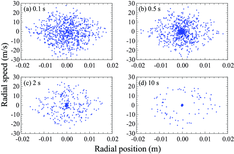
Figure 8: (Color online) Simulated time evolution of the radial phase-space distributions of molecules in the microwave trap overlapped with a 140 $\mu$K atom cloud with a width of $w_{a}=3$ mm. The cooling times are (a) 0.1 s, (b) 0.5 s (c) 2 s and (d) 10 s.

Figure 8 shows how the distribution of molecules in the trap evolves with time as they cool to the temperature of the atom cloud whose width is $w_{a}=3$ mm. Each plot shows the radial position and speed of each molecule in the trap. After 0.1 s very little cooling has occurred and the molecules have the full range of speeds and positions that the trap can accept. After 0.5 s it is clear that the molecules are accumulating near the phase-space origin as expected. They have small speeds and are confined near the centre of the trap. As time goes on, the accumulation of cold molecules continues. After 2 s the majority of the molecules have been cooled into the small area of phase space near the origin, but some molecules remain distributed throughout the phase-space acceptance. The distribution has separated into two components, one cold and one hot. After 10 s, 90% of the molecules are in the cold component, the remaining hot molecules form a halo in phase space around the cold ones, and there is a region in between where there are no molecules at all. The molecules that are slow to cool are the ones that initially have large angular momentum about the trap centre. In the absence of collisions, these molecules cannot reach the centre, and if they cannot reach the centre they are unlikely to have any collisions. The molecules in the halo in Figure 8(d) have particularly large angular momenta and so spend all their time in the far wings of the atomic distribution; they are unlikely to have collisions even after 10 s.

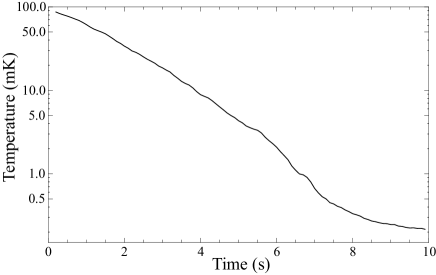
Figure 9: Temperature versus time for molecules thermalizing with cold atoms in a microwave trap. The atom distribution has a temperature of $T_{a}=140\,\mu$K and a width of $w_{a}=5$ mm. To obtain the molecule temperature, we take the kinetic energy distribution, remove high energy outliers, take the mean and divide by $\frac{3}{2}k$.

The two-component speed distribution is even more evident when the atom cloud width is reduced to 1 mm. In this case, a cold distribution develops rapidly at the centre of the trap but the rest of the trap phase-space acceptance is filled with hot molecules, apart from a thin empty region separating the hot and cold distributions. When the atom cloud width is $w_{a}=5$ mm the atom-molecule overlap is sufficient that the molecules form a single-component speed distribution. In this case it is possible to give a sensible measure of the temperature. The mean kinetic energy is not a good measure because a few remaining outliers with high kinetic energy have a disproportionate effect on the mean. Instead, we trim the distribution by removing the 5% that have the highest kinetic energy, take the mean, and then divide by $\frac{3}{2}k$ to obtain a temperature. Figure 9 shows the result. After 10 s the molecules have cooled from an initial temperature of 100 mK to a final temperature of 200 $\mu$K, close to the temperature of the atom cloud. The mean number of collisions per molecule required to reach this temperature is 30. As the molecules cool they move into the densest part of the atomic distribution and, as shown in Figure 1, the collision cross section tends to increase. As a result, the cooling rate tends to increase gradually between 100 mK and 1 mK, despite the fact that the collision rate is proportional to the decreasing speed.

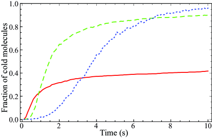
Figure 10: (Color online) Fraction of cold molecules in the simulated microwave trap as a function of time, for three different atom cloud sizes: 1 mm (red solid line), 3 mm (green dashed line) and 5 mm (blue dotted line). A molecule is classified as cold if its kinetic energy is less than $\frac{3}{2}kT$, where $T=1$ mK.

Figure 10 shows the number of cold molecules as a function of time for three different atomic cloud sizes. The number of molecules is normalized to the total number in the trap, and a molecule is taken to be cold once its kinetic energy is less than $\frac{3}{2}kT$, where $T=1$ mK. When $w_{a}=5$ mm, almost all the molecules in the trap cool to low temperature, but the cooling is slow because the atom density is low. After 1 s, only 2% of the molecules are cold, but after 10 s, 96% of them are cold. As the atomic density is increased by reducing the size of the cloud, the cooling rate at early times increases. However, the number of cold molecules obtained after a long period of cooling is lower with these smaller atom clouds. For both the 1 mm and 3 mm atom clouds, about 25% of the molecules are cold after 1 s. After 10 s, 90% of the molecules are cold when $w_{a}=3$ mm, but only 42% when $w_{a}=1$ mm. As discussed above, the molecules that fail to cool are those that have large angular momentum about the centre of the trap. These results show that the most suitable choice of atom cloud size depends on the trap lifetime. If the lifetime is long enough, it is best to use a large atom cloud to maximize the number of cold molecules obtained. If the lifetime is short, it is better to use a small atom cloud to maximize the cooling rate and then to remove the molecules that remain hot, for example by lowering the trap depth.

IV Conclusions

Molecules are most easily trapped when they are prepared in weak-field-seeking states, but then sympathetic cooling is feasible only if the ratio of elastic to inelastic cross sections is high. In the Li+LiH system with LiH in its rotationally excited state ($j=1$), we find this ratio to be approximately 5 at a collision energy of 100 mK, gradually falling as the collision energy decreases and reaching 1 at about 30 $\mu$K. This ratio is too small for sympathetic cooling to be effective, since cooling from 100 mK to 100 $\mu$K results in 4 orders of magnitude of trap loss. To avoid inelastic losses in this system, the molecules need to be trapped in the ground state. This can be done using an ac electric trap, but in this trap collisions can transfer stable molecules onto unstable trajectories. This occurs because stability of motion in an ac trap relies on a specific correlation between position and speed, and this necessary correlation tends to be upset by collisions. Our simulations suggest that the resulting trap losses are too great for sympathetic cooling to be feasible in a realistic ac trap.

Alternatively, ground-state molecules can be trapped in the electric field maximum of a standing wave microwave field formed inside a microwave cavity. The microwave trap appears to be suitable for sympathetic cooling. We find that both the cooling rate and the fraction of molecules that cool depend on the degree of overlap between the atom and molecule distributions. When the atoms are compressed to a small volume, the cooling rate is high at the trap centre, but a large fraction of the molecules do not cool because their angular momentum prevents them from reaching the centre of the trap. When the atom cloud is larger, more of the molecules cool but the cooling is slower. The typical time required for a large fraction of the molecules to reach ultracold temperatures is a few seconds. For ground-state LiH, in a good vacuum, the trap lifetime will be limited by black-body heating of the rotational motion Hoekstra07 . This black-body-limited lifetime is 2.1 s at room temperature, rising to 9.1 s at 77 K Buhmann08 . This suggests that liquid nitrogen cooling of the microwave cavity may be necessary in order to cool a large fraction of the molecules in the time available. Cooling of the cavity mirrors would also allow for a factor of 10 increase in the cavity Q-factor, and a corresponding decrease in the power required to obtain the same trap depth. Note that the black-body heating rate is considerably slower for many other molecules of interest Hoekstra07 ; Buhmann08 , and then trap lifetimes of several tens of seconds should be attainable under good vacuum conditions.

Our use of a hard-sphere scattering model may underestimate the degree of forward scattering, thereby overestimating the cooling rate since scattering in the forward direction does little to cool the molecules. We will investigate this in future work. We have used an unchanging atomic distribution in our simulations, but it is clear that the atoms could be used more efficiently. It would be better to compress the atom cloud gradually so that the size of the atom distribution matches that of the molecules as they cool towards the trap centre. This optimizes the collision rate by optimizing the atom density and the overlap between the two clouds at all times. Compressing the atom cloud will raise its temperature, but at high densities the atoms can be evaporatively cooled which will in turn sympathetically cool the molecules to even lower temperatures. We have focussed on LiH molecules sympathetically cooled with Li atoms, but we expect our general conclusions to apply to a wide range of other systems.

- (1)
- (2) L. D. Carr, D. DeMille, R. V. Krems and J. Ye, New. J. Phys. 11, 055049 (2009).
- (3) A. Micheli, G. K. Brennen and P. Zoller, Nature Physics 2, 341 (2006).
- (4) R. V. Krems, Int. Rev. Phys. Chem. 24, 99 (2005).
- Hudson et al. (2002) J. J. Hudson, B. E. Sauer, M. R. Tarbutt, and E. A. Hinds, Phys. Rev. Lett. 89, 023003 (2002).
- Hudson et al. (2006) E. R. Hudson, H. J. Lewandowski, B. C. Sawyer, and J. Ye, Phys. Rev. Lett. 96, 143004 (2006).
- Bethlem et al. (2008) H. L. Bethlem, M. Kajita, B. Sartakov, G. Meijer, and W. Ubachs, Eur. Phys. J. Special Topics 163, 55 (2008).
- Bethlem and Ubachs (2009) H. L. Bethlem and W. Ubachs, Faraday Disscus. 142, 25 (2009).
- DeMille et al. (2008) D. DeMille, S. B. Cahn, D. Murphree, D. A. Rahmlow, and M. G. Kozlov, Phys. Rev. Lett. 100, 023003 (2008).
- Darquié et al. (2010) B. Darquié, C. Stoeffler, A. Shelkovnikov, C. Daussy, A. Amy-Klein, C. Chardonnet, S. Zrig, L. Guy, J. Crassous, P. Soulard, et al., ArXiv e-prints (2010), eprint 1007.3352.
- Tarbutt et al. (2009b) M. R. Tarbutt, J. J. Hudson, B. E. Sauer, and E. A. Hinds, Faraday Discuss. 142, 370 (2009b).
- (12) J. M. Sage, S. Sainis, T. Bergeman and D. DeMille, Phys. Rev. Lett. 94, 203001 (2005).
- (13) J. Deiglmayr, A. Grochola, M. Repp, K. Mörtlbauer, C. Glück, J. Lange, O. Dulieu, R. Wester and M. Weidemüller, Phys. Rev. Lett. 101, 133004 (2008).
- (14) S. Ospelkaus, A. Pe’er, K. -K. Ni, J. J. Zirbel, B. Neyenhuis, S. Kotochigova, P. S. Julienne, J. Ye and D. S. Jin, Nature Phys. 4, 622 (2008).
- (15) F. Lang, K. Winkler, C. Strauss, R. Grimm and J. Hecker Denschlag, Phys. Rev. Lett. 101, 133005 (2008).
- (16) J. G. Danzl, E. Haller, M. Gustavsson, M. J. Mark, R. Hart, N. Bouloufa, O. Dulieu, H. Ritsch and H. C. Nägerl, Science 321, 1062 (2008).
- (17) J. G. Danzl, M. J. Mark, E. Haller, M. Gustavsson, R. Hart, J. Aldegunde, J. M. Hutson and H. C. Nägerl, Nature Phys. 6, 265 (2010).
- (18) E. S. Shuman, J. F. Barry and D. DeMille, Nature 467, 820 (2010).
- (19) H. L. Bethlem, G. Berden and G. Meijer, Phys. Rev. Lett. 83, 1558 (1999).
- (20) E. Narevicius, A. Libson, C. G. Parthey, I. Chavez, J. Narevicius, U. Even and M. Raizen, Phys. Rev. A 77, 051401(R) (2008).
- (21) R. Fulton, A. I. Bishop, M. N. Schneider and P. F. Barker, Nature Phys. 2, 465 (2006).
- (22) J. D. Weinstein, R. deCarvalho, T. Guillet, B. Friedrich and J. M. Doyle, Nature 395, 148 (1998).
- (23) L. D. van Buuren, C. Sommer, M. Motsch, S. Pohle, M. Schenk, J. Bayerl, P. W. H. Pinkse and G. Rempe, Phys. Rev. Lett. 102, 033001 (2009).
- (24) C. J. Myatt, E. A. Burt, R. W. Ghrist, E. A. Cornell and C. E. Wieman, Phys. Rev. Lett. 78, 586 (1997).
- (25) A. G. Truscott, K. E. Strecker, W. I. McAlexander, G. B. Partridge and R. G. Hulet, Science 291, 2570 (2001).
- (26) G. Modugno, G. Ferrari, G. Roati, R. J. Brecha, A. Simoni and M. Inguscio, Science 294, 1320 (2001).
- (27) D. J. Larson, J. C. Bergquist, J. Bollinger, W. M. Itano and D. J. Wineland, Phys. Rev. Lett. 57, 70 (1986).
- (28) M. Drewsen, A. Mortensen, R. Martinussen, P. Staanum and J. L. Sørensen, Phys. Rev. Lett. 93, 243201 (2004).
- (29) A. Ostendorf, C. B. Zhang, M. A. Wilson, D. Offenberg, B. Roth and S. Schiller, Phys. Rev. Lett. 97, 243005 (2006).
- (30) S.K. Tokunaga, J. J. Hudson, B. E. Sauer, E. A. Hinds and M. R. Tarbutt, J. Chem. Phys. 126, 124314 (2007).
- (31) S. K. Tokunaga, J. M. Dyne, E. A. Hinds and M. R. Tarbutt, New J. Phys. 11, 055038 (2009).
- (32) M. Lara, J. L Bohn, D. Potter, P.Soldán and J. M. Hutson, Phys. Rev. Lett. 97, 183201 (2006).
- Skomorowski et al. (2010) W. Skomorowski, F. Pawłowski, T. Korona, R. Moszynski, P. S. Żuchowski, and J. M. Hutson, arXiv:1009:4312 (2010).
- Hutson and Green (1994) J. M. Hutson and S. Green, MOLSCAT computer program, version 14, distributed by Collaborative Computational Project No. 6 of the UK Engineering and Physical Sciences Research Council (1994).
- Alexander and Manolopoulos (1987) M. H. Alexander and D. E. Manolopoulos, J. Chem. Phys. 86, 2044 (1987).
- Soldán et al. (2009) P. Soldán, P. S. Żuchowski, and J. M. Hutson, Faraday Discuss. 142, 191 (2009).
- Żuchowski and Hutson (2009) P. S. Żuchowski and J. M. Hutson, Phys. Rev. A 79, 062708 (2009).
- Wigner (1948) E. P. Wigner, Phys. Rev. 73, 1002 (1948).
- Gribakin and Flambaum (1993) G. F. Gribakin and V. V. Flambaum, Phys. Rev. A 48, 546 (1993).
- (40) P. Barletta, J. Tennyson and P. F. Barker, New J. Phys. 12, 113002 (2010).
- (41) L. P. Parazzoli, N. J. Fitch, P. S. Żuchowski, J. M. Hutson and H. J. Lewandowski, arXiv:1101.2886 (2011).
- (42) J. van Veldhoven, H. L. Bethlem and G. Meijer, Phys. Rev. Lett. 94, 083001 (2005).
- (43) H. L. Bethlem, J. van Veldhoven, M. Schnell and G. Meijer, Phys. Rev. A 74, 063403 (2006).
- (44) M. Schnell, P. Lützow, J. van Veldhoven, H. L. Bethlem, J. Küpper, B. Friedrich, M. Schleier-Smith, H. Haak and G. Meijer, J. Phys. Chem. A 111, 7411 (2007).
- (45) S. Schlunk, A. Marian, P. Geng, A. P. Mosk, G. Meijer and W. Schöllkopf, Phys. Rev. Lett. 98, 223002 (2007).
- (46) T. Rieger, P. Windpassinger, S. A. Rangwala, G. Rempe and P. W. H. Pinkse, Phys. Rev. Lett. 99, 063001 (2007).
- (47) D. DeMille, D. R. Glenn and J.Petricka, Eur. Phys. J. D 31, 375 (2004).
- (48) S. V. Alyabyshev, T. V. Tscherbul and R. V. Krems, Phys. Rev. A 79, 060703(R) (2009).
- (49) S. Hoekstra, J. J. Gilijamse, B. Sartakov, N. Vanhaecke, L. Scharfenberg, S. Y. T. van de Meerakker and G. Meijer, Phys. Rev. Lett. 98, 133001 (2007).
- (50) S. Y. Buhmann, M. R. Tarbutt, S. Scheel and E. A. Hinds, Phys. Rev. A 78, 052901 (2008).