Spectral decomposition of entangled photons with an arbitrary pump

Abstract

We calculate the bi-photon state generated by spontaneous parametric down conversion in a thin crystal and under collinear phase matching conditions using a pump consisting of any superposition of Laguerre-Gauss modes. The result has no restrictions on the angular or radial momenta or, in particular, on the width of the pump, signal and idler modes. We demonstrate the strong effect of the pump to signal/idler width ratio on the composition of the down-converted entangled fields. Knowledge of the pump to signal/idler width ratio is shown to be essential when calculating the maximally entangled states that can be produced using pumps with a complex spatial profile.

1 Introduction

Quantum entanglement is one of the defining properties of quantum mechanics. It forms the basis for quantum information [1, 2] and quantum computing [3] and is essential for applications such as entangled cryptographic systems [4] and quantum imaging [5, 6, 7, 8]. Much of the research in this area has focussed on qubit quantum entanglement, although entanglement has also been demonstrated between spatial modes carrying orbital angular momentum (OAM) [9, 10, 11]. Since these modes are defined within an infinite-dimensional, discrete Hilbert space there is considerable interest in their potential to generate multi-dimensional entangled states not only for enhancing the efficiency of current quantum protocols, but also for the realization of new, higher dimensional quantum channels.

Spontaneous parametric down conversion (SPDC), the generation of two lower-frequency photons when a pump field interacts with a nonlinear crystal, has been shown to be a reliable source of photons which are entangled [12] and, in particular, in their OAM [9]. The spatial structure of the down-converted biphotons can be expressed as a superposition of Laguerre-Gauss modes of different amplitudes, with the width of the modal expansion relating to the amount of entanglement of the final state. In this paper, we calculate the exact analytical form of the biphotons for any Laguerre-Gauss pump, with no restrictions on the angular or radial momenta, $\ell$ and $p$, respectively, or, in particular, on the width, $w$, of the pump, signal and idler modes. Our calculation demonstrates that OAM is conserved.

We use our result to calculate the coincidence amplitudes of the LG modes in the generated two-photon entangled state for a variety of pump beams. We demonstrate the the importance of the various beam sizes (the pump width and the choice of LG base for the signal and idler) in determining the state of the down-converted photon and the resulting $\ell$ distribution, also known as the quantum spiral bandwidth (SB) [13]. We find excellent agreement with previous analyses which considered more restricted conditions [13, 14].

Knowledge of the exact form of the down-converted photons opens up the possibility of engineering the entangled modes, through an appropriate choice of pump beam, in order to produce biphotons which are, for example, maximally entangled in some subspace [15]. We show how our result can be easily extended to pump beams which are complex superpositions of Laguerre-Gauss modes, including pump modes containing phase singularities. We again see excellent agreement with previous analysis [15]. Moreover, by allowing the beam widths to be free parameters, we show that the pump to signal/idler size plays a critical role in the engineering of the down-converted state, with states only being maximally entangled at particular width ratios.

2 Spontaneous parametric down conversion and spiral bandwidth

We consider a thin nonlinear crystal (typically $1$–$3$mm), tuned for type-I, collinear down-conversion, illuminated by a continuous-wave Laguerre-Gaussian pump beam propagating in the $z$-direction and confined within the crystal and assume perfect phase matching. This produces two highly-correlated, lower-frequency photons, commonly termed signal and idler. Since energy is conserved, $\omega_{p}=\omega_{s}+\omega_{i}$, where the subscripts $p,s,i$ refer to the pump, signal and idler, respectively.

The down-converted biphoton state in this case is given by [16, 15]

$$|\psi_{SPDC}\rangle=\int dr_{\perp}\Phi(r_{\perp})\hat{a}_{s}^{\dagger}(r_{\perp})\hat{a}_{i}^{\dagger}(r_{\perp})|0,0\rangle$$ (1)

where $\Phi(r_{\perp})$ is the spatial distribution of the pump beam at the input face of the crystal, $|0,0\rangle$ is the vacuum state and $\hat{a}_{s}^{\dagger}(r_{\perp})$, $\hat{a}_{i}^{\dagger}(r_{\perp})$ are creation operators for the signal and idler modes, respectively. The integral is over the plane perpendicular to the axis of the pump beam.

Since the photon pairs generated by SPDC are entangled in arbitrary superpositions of an infinite number of modes with OAM they are best described by mode functions that are Laguerre-Gauss modes, $LG_{p}^{\ell}$. At the beam waist ($z=0$) the normalised LG modes are given, in cylindrical co-ordinates, by [17]:

$$LG_{p}^{\ell}(\rho,\phi)=\sqrt{\frac{2p!}{\pi\left(p+|\ell|\right)!}}\frac{1}{w}\left(\frac{\rho\sqrt{2}}{w}\right)^{|\ell|}\exp\left(\frac{-\rho^{2}}{w^{2}}\right)L_{p}^{|\ell|}\left(\frac{2\rho^{2}}{w^{2}}\right)\exp(i\ell\phi).$$ (2)

Here $w$ is the beam waist, $\ell$ corresponds to the angular momentum, $\ell\hbar$, carried by the beam and describes the helical structure of the wave front around a wave front singularity and $p+1$ describes the number of radial intensity maxima.

We can then write the biphoton state as:

$$|\psi_{SPDC}\rangle=\sum_{\ell_{s},p_{s}}\sum_{\ell_{i},p_{i}}C_{p_{s},p_{i}}^{\ell_{s},\ell_{i}}\left|\ell_{s},p_{s};\ell_{i},p_{i}\right\rangle$$ (3)

where $P_{p_{s},p_{i}}^{\ell_{s},\ell_{i}}=\left|C_{p_{s},p_{i}}^{\ell_{s},\ell_{i}}\right|^{2}$ is the probability of finding one photon in the signal mode $\left|\ell_{s},p_{s}\right\rangle$ and the other in the idler mode $\left|\ell_{i},p_{i}\right\rangle$ given a pump mode $\left|\ell_{p},p_{p}\right\rangle$.

The coincidence amplitudes $C_{p_{s},p_{i}}^{\ell_{s},\ell_{i}}$ are calculated from the overlap integral

$$C_{p_{s},p_{i}}^{\ell_{s},\ell_{i}} = \langle\psi_{i},\psi_{s}|\psi_{SPDC}\rangle$$ (4)

$$= \int_{0}^{2\pi}d\phi\int_{0}^{\infty}\rho\,d\rho LG_{p_{p}}^{\ell_{p}}(\rho,\phi)\left[LG_{p_{s}}^{l_{s}}(\rho,\phi)\right]^{*}\left[LG_{p_{i}}^{l_{i}}(\rho,\phi)\right]^{*}.$$ (5)

Note that after substituting (2) into (5) the integral over the azimuthal coordinate is

$$\int_{0}^{2\pi}\,\,d\phi\exp\left[i\left(\ell_{p}-\ell_{s}-\ell_{i}\right)\phi\right]=2\pi\delta_{\ell_{p},\ell_{s}+\ell_{i}},$$ (6)

from which we obtain the well-known conservation law for the orbital angular momentum: $\ell_{p}=\ell_{s}+\ell_{i}$ [9, 18]. Substituting this into (5), and making use of the associated Laguerre polynomial in the form [19]

$$L_{p}^{|\ell|}(x)=\sum_{i=0}^{p}(-1)^{i}\frac{(p+|\ell|)!}{(p-i)!(|\ell|+i)!i!}\,x^{i}\,,$$ (7)

we obtain

$$C_{p_{s},p_{i}}^{\ell_{s},\ell_{i}} = \delta_{\ell_{p},\ell_{s}+\ell_{i}}\sqrt{\frac{2}{\pi w_{p}^{2}}}\,\frac{2^{\sigma_{\ell}+1}\gamma_{s}^{|\ell_{s}|+1}\gamma_{i}^{|\ell_{i}|+1}}{\left(1+\gamma_{s}^{2}+\gamma_{i}^{2}\right)^{\sigma_{\ell}+1}}$$ (8)

$$\times \sqrt{p_{p}!p_{s}!p_{i}!\left(|\ell_{p}|+p_{p}\right)!\left(|\ell_{s}|+p_{s}\right)!\left(|\ell_{i}|+p_{i}\right)!}$$

$$\times \sum_{k=0}^{p_{p}}\sum_{i=0}^{p_{s}}\sum_{j=0}^{p_{i}}\frac{(-2)^{k+i+j}\gamma_{s}^{2i}\gamma_{i}^{2j}}{\left(1+\gamma_{s}^{2}+\gamma_{i}^{2}\right)^{k+i+j}}$$

$$\times \frac{\left[\sigma_{\ell}+k+i+j\right]!}{(p_{p}-k)!(|\ell_{p}|+k)!k!(p_{s}-i)!(|\ell_{s}|+i)!i!(p_{i}-j)!(|\ell_{i}|+j)!j!},$$

where $\sigma_{\ell}=\left(|\ell_{p}|+|\ell_{s}|+|\ell_{i}|\right)/2$ and $\gamma_{s}=w_{p}/w_{s}$, $\gamma_{i}=w_{p}/w_{i}$ are the ratios of the pump width to the signal/idler widths.

Equation (8) allows us to calculate the exact analytical form of the down-converted photons produced using any Laguerre-Gaussian pump (or superposition thereof) with no restrictions on any of the beam parameters. Calculation of the coincidence amplitudes can also be used to calculate the number of OAM modes participating in the down-converted state, otherwise known as the spiral bandwidth (SB).

3 Coincidence amplitudes and spiral bandwidth for special cases

For a given pump, equation (8) shows that the coincidence amplitudes have a strong dependence on the ratio of the pump width to the chosen widths of the LG bases for the signal and idler, $\gamma_{s}$ and $\gamma_{i}$. Experimentally, the maximum width of the pump is limited by the size of the down-conversion crystal, while the widths of the signal and idler beams are determined by the size of the single mode fibre used in the detection process. We can see this dependence more clearly if we consider some simplified examples.

3.1 Gaussian pump, $\ell_{p}=p_{p}=0$.

We first consider the simplest possible case: a Gaussian pump with $\ell_{p}=p_{p}=0$ and biphotons with no radial dependence i.e. $p_{s}=p_{i}=0$. Moreover, we assume that the signal and idler modes have the same width s.t. $\gamma_{s}=\gamma_{i}=\gamma$. From from conservation of OAM, equation (6), we know that $\ell_{s}=-\ell_{i}=\ell$ in this case and so we can reduce equation (8) to

$$C_{0,0}^{\ell,-\ell}=\sqrt{\frac{2}{\pi w_{p}^{2}}}\,\left(\frac{2\gamma^{2}}{1+2\gamma^{2}}\right)^{|\ell|+1}.$$ (9)

It is clear that the SB depends only on the ratio of the pump to signal/idler widths, $\gamma$. As in previous work, for example [13, 14], this further reduces to

$$C_{0,0}^{\ell,-\ell}\propto\left(\frac{2}{3}\right)^{|\ell|}$$ (10)

when all the beam widths are the same, i.e. $\gamma=1$.

The effect of $\gamma$ on the spiral bandwidth is shown in figure (1) where we have plotted the SB as a function of $\gamma$. It can be seen that as the signal/idler widths are reduced w.r.t. the pump width (i.e. as $\gamma$ increases) the SB increases but that the amplitudes of the participating modes decrease. In figure (2) we plot (in blue) the SBs for $\gamma=1.0,2.0$ and $3.0$. These results are in excellent agreement with previous work, see, for example, figure (1) of [13] (shown in red in figure (2)). Note that throughout this work although we only plot the SB from $-15\leq\ell\leq 15$, which are experimentally realisable values, we calculate the coincidence amplitudes for a much larger range of $\ell$ and use these results to “normalize” the coincidence probabilities.

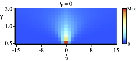
Figure 1: Spiral bandwidth for a Gaussian pump, $\ell_{p}=p_{p}=0$ and fixed width $w_{p}=1.0$ as a function $\gamma$.

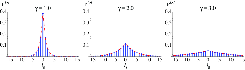
Figure 2: Spiral bandwidth for a Gaussian pump, $\ell_{p}=p_{p}=0,w_{p}=1.0$. The signal and idler widths are equal and reduced s.t. $\gamma=1.0,2.0,3.0$ from left to right. Vertical (blue) lines are calculated using (9) and dashed (red) lines are calculated using eqn.s (10) & (11) of [13].

The effect of the different beam parameters with a Gaussian pump has recently been explored [20]. Note that the results are also valid for non-collinear geometries in the approximation of a thin crystal.

3.2 Laguerre-Gaussian pump, $\ell_{p}>0$.

We now consider what happens when the pump is a higher-order Laguerre-Gaussian mode, i.e. $\ell_{p}>0$. In this case conservation of OAM requires $\ell_{i}=\ell_{p}-\ell_{s}$. As before, we start with the simplest case: $p_{p,s,i}=0$ and assume that the signal and idler modes have the same width. The probability amplitudes are then described by

$$C_{0,0}^{\ell_{s},\ell_{i}}=\delta_{\ell_{p},\ell_{s}+\ell_{i}}\sqrt{\frac{2}{\pi w_{p}^{2}}}\frac{2^{\sigma_{\ell}+1}\sigma_{\ell}!}{\sqrt{|\ell_{p}|!|\ell_{s}|!|\ell_{i}|!}}\frac{\gamma_{s}^{|\ell_{s}|+1}\gamma_{i}^{|\ell_{i}|+1}}{\left(1+\gamma_{s}^{2}+\gamma_{i}^{2}\right)^{\sigma_{\ell}+1}}$$

where $\sigma_{\ell}=\left(|\ell_{p}|+|\ell_{s}|+|\ell_{i}|\right)/2$. This agrees with equation (8) of [14] when using normalized LG modes and assuming that all of the modes have the same width.

To see how the OAM of the pump affects the spiral bandwidth we first calculate the coincidence probabilities, $P_{0,0}^{\ell_{s},\ell_{p}-\ell_{s}}$, as a function of $\ell_{s}$ and $\gamma$ for different values of $\ell_{p}$. As figure (3) shows, the SB is symmetric around the OAM value of the pump. For small values of $\gamma$ the SB has a maximum at $\ell_{s}=\ell_{p}$. As $\gamma$ is increased, however, the SB splits into two “wings” for $\ell_{p}>0$, with a minimum at $\ell_{s}=\ell_{p}$, and the amplitude increasing with $\ell_{s}$. The physical explanation of this is that pump modes with $\ell_{p}>0$ form a rings whose diameter increases with both the value of $\ell_{p}$ and the width of the beam. Maximum overlap between the pump and the signal/idler modes, and hence maximum coincidence amplitudes, therefore occurs for larger values of $\ell_{s},\ell_{i}$.

We next consider what happens if the widths of the signal and idler are different. We find that by varying the ratio of the signal to idler widths (in this case from $\gamma_{i}=0.5\gamma_{s}$ to $2.0\gamma_{s}$) it is possible to fully suppress the SB for either negative or positive values of $\ell_{s}$, as shown in figure (4).

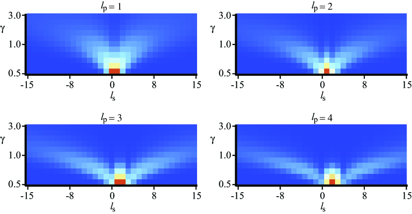
Figure 3: Spiral bandwidth for a Laguerre-Gaussian pumps of fixed width $w_{p}=1.0$ and $\ell_{p}=1,2,3,4$ as the signal/idler width is reduced s.t. $\gamma_{s}=\gamma_{i}$ goes from $0.5$ to $3.0$.

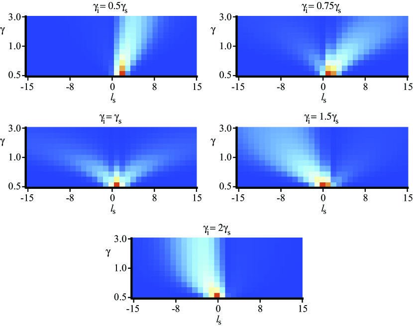
Figure 4: Spiral bandwidth for a Laguerre-Gaussian pump with $\ell_{p}=2,w_{p}=1.0$ as the signal/idler width is reduced s.t. $\gamma_{s}$ goes from $0.5$ to $3.0$. The signal and idler modes have different width ratios $\gamma_{i}/\gamma_{s}=0.5,0.75,1.0,1.5,2.0$.

Until now we have considered only modes with no radial modes, i.e. $p_{p}=p_{s}=p_{i}=0$. Higher-order LG beams are commonly produced using a spatial light modulator (SLM). Since these produce OAM modes with a range of radial indices, $p$, [21], we now look at the effect $p$ has on the form of the spatial mode function of the entangled photons. We find that the number of “wings” increases with the radial index of the pump as shown in figure (5). As before, altering the ratio of the signal to idler width suppresses one set of wings. Again these correspond to areas of maximum overlap between the pump and the signal/idler modes.

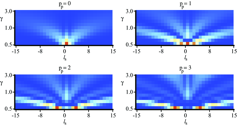
Figure 5: Spiral bandwidth for a Laguerre-Gaussian pumps with $\ell_{p}=2,w_{p}=1.0$ as the signal/idler width is reduced s.t. $\gamma_{s}=\gamma_{i}$ goes from $0.5$ to $3.0$. The radial number of the pump is increased from $p_{p}=0$ to $3$.

If we allow first our signal/idler beams to have non-zero radial modes and then all beams to have non-zero radial modes the spiral bandwidth as a function of $\gamma$ becomes ever more complex. The effect of the radial number of the pump is shown in figure (6).

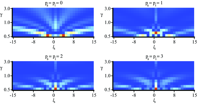
Figure 6: Spiral bandwidth for a Laguerre-Gaussian pumps with $\ell_{p}=p_{p}=2,w_{p}=1.0$ as the signal/idler width is reduced s.t. $\gamma_{s}=\gamma_{i}$ goes from $0.5$ to $3.0$. The radial number of the signal and idler modes is increased from $p_{s}=p_{i}=0$ to $3$.

3.3 Engineered entangled states

For many quantum communication applications entangling systems in higher-dimensional states is important. Not only does the higher dimensionality imply a greater potential for applications in quantum information processing, but it has also been suggested that increasing the dimensionality of the entangled states of a system can make its non-classical correlations more robust to the presence of noise and other detrimental effects [22, 23]. Torres et al. demonstrated (theoretically) that arbitrary engineered entangled states in any $d$-dimensional Hilbert space can be prepared using SPDC to translate the topological information contained in a pump beam into the amplitudes of the generated entangled quantum states [15]. Controlling OAM state superpositions in this way engenders the ability to produce and manipulate quantum states with an arbitrarily large number of dimensions. Indeed, Torres et al. illustrated this by calculating a number of maximally entangled states of different dimensions, produced using pump beams containing phase singularities (PS). Here we describe how our results can be easily extended to such pumps, which can be described by complex superpositions of LG modes [24]. Moreover, we demonstrate that the ratio of the pump to signal/idler widths must be taken into consideration in the calculation as it plays a critical role in the composition of the down-converted state: a state is generally maximally entangled for only one pump to signal/idler width ratio.

We first calculate the coincidence amplitudes resulting from a pump that is a superposition of Laguerre-Gauss modes of equal width, $w_{p}$, and complex amplitudes $a_{n}$. We can write this as

$$\sum_{n}a_{n}LG_{p_{n}}^{\ell_{n}}(\rho,\phi)=a_{1}LG_{p_{1}}^{\ell_{1}}(\rho,\phi)+a_{2}LG_{p_{2}}^{\ell_{2}}(\rho,\phi)+\ldots$$ (11)

where $n$ labels the modes in the superposition and $\sum_{n}|a_{n}|^{2}=1$. The overlap integral (5) then becomes

$$C_{p_{s},p_{i}}^{\ell_{s},\ell_{i}} = \sum_{n}\int_{0}^{2\pi}d\phi\int_{0}^{\infty}\rho\,d\rho a_{n}LG_{p_{n}}^{\ell_{n}}(\rho,\phi)\left[LG_{p_{s}}^{l_{s}}(\rho,\phi)\right]^{*}\left[LG_{p_{i}}^{l_{i}}(\rho,\phi)\right]^{*}$$ (12)

$$= \sum_{n}a_{n}C_{n,p_{s},p_{i}}^{\;\;\;\,\ell_{s},\ell_{i}},$$

where $C_{n,p_{s},p_{i}}^{\;\;\;\,\ell_{s},\ell_{i}}$ are the coincidence amplitudes, calculated from (8), for each Laguerre-Gaussian component, $\left|\ell_{p},p_{p}\right\rangle$, of the pump field.

In order to investigate a pump containing PSs we make use of its projection onto LG modes [25]. A field containing $N$ PSs can be written as a superposition of LG modes, $\sum_{\ell=0}^{N}a_{\ell}LG_{0}^{\ell}$, with complex amplitudes

$$a_{\ell}=\sqrt{\pi}(-1)^{N-\ell}\left(\frac{w_{p}}{\sqrt{2}}\right)^{\ell-1}\sqrt{\ell!}\,\,b_{N-\ell}$$ (13)

where $b_{n}$ are given by equation (11) of [15] or, equivalently, by

$$b_{n}=\frac{1}{m!}\frac{\partial^{m}}{\partial x^{m}}\prod_{i=1}^{N}\left(1+\rho_{i}e^{i\phi_{i}}x\right)\big{|}_{x=0}$$ (14)

with $m=[0,N]$ and $\rho_{i},\phi_{i}$ being the radial and azimuthal positions of the PSs, respectively.

Following [15], we consider a pump containing six PSs at positions $\rho_{1}=0.65w_{p},\,\rho_{2}=1.85w_{p},\,\rho_{3}=1.06w_{p},\,\rho_{4}=0.54w_{p},\,\rho_{5}=1.53w_{p},\,\rho_{6}=1.24w_{p}$ and $\phi_{i}=i\pi/3$ for $i=1,6$. Substituting these values into (13) and then into (12) allows us to calculate the form of the pump, as shown on the left in figure (7), and the resultant coincidence probabilities, vertical (blue) lines shown on the right in figure (7). We find excellent agreement with the results from eqn. (14) of [15] (dashed red line). We calculated the coincidence probabilities $P_{0,0}^{0,0},P_{0,0}^{1,1},P_{0,0}^{2,2},P_{0,0}^{3,3}$ and confirmed that these were equal and so this pump produces the maximally entangled qu-quart in the subspace $S_{4}=\{\left|0,0\right>,\left|1,1\right>,\left|2,2\right>,\left|3,3\right>\}$.

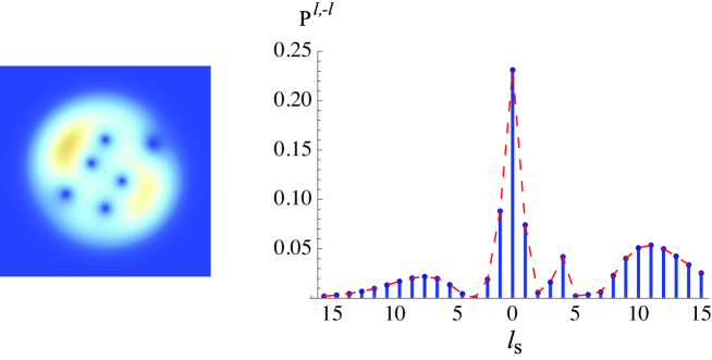
Figure 7: Pump containing six phase singularities, as described in [15], and resulting probability amplitudes. The blue lines show the results found using equation (14) of [15] while the red line is the result found using equations (8) and (12).

Note, however, that in this example we assumed that the pump, signal and idler all had the same width i.e. $\gamma_{s}=\gamma_{i}=1$. Since we have seen that the composition of the down-converted state is strongly dependent on the ratio of the pump to signal and idler widths we extended these results by calculating the spiral bandwidth as a function of $\gamma$, keeping $\gamma_{s}=\gamma_{i}$ for simplicity. As expected, we see a large variation in SB for different $\gamma$, as shown on the left in figure (8). This can been seen more clearly on the right of figure (8), where we plot the SB at $\gamma=1.0,2.0,3.0$. It is clear that by choosing the mode widths appropriately it is possible to tailor the spiral bandwidth in very different ways.

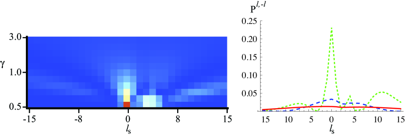
Figure 8: Spiral bandwidth for superposition pump for $\gamma_{s}=\gamma_{i}=0.5$ to $3.0$ (left) with slices at $\gamma_{s}=\gamma_{i}=1.0$ (green, small dash), $2.0$ (blue, large dash) and $3.0$ (red, solid) shown on right.

Changing the relative beam sizes has a large effect on the composition of the entangled state with important implications in the “engineering” of the down-converted state: states which are maximally entangled for one value of $\gamma$ are generally not maximally entangled for any other values of $\gamma$ values. To illustrate this we consider the maximally entangled qu-quart produced by the six-PS pump above and calculate the coincidence probabilities $P_{0,0}^{0,0},P_{0,0}^{1,1},P_{0,0}^{2,2},P_{0,0}^{3,3}$ as a function of $\gamma$. From figure (9) it is clear that this state is only maximally entangled if $\gamma=0.5$ or $\gamma=1.0$. In order to obtain this state then, one has to ensure that these conditions are met.

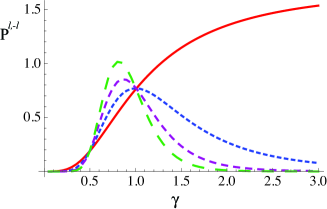
Figure 9: Coincidence probabilities $P_{0,0}^{0,0}$ (red, solid), $P_{0,0}^{1,1}$ (blue, small dash), $P_{0,0}^{2,2}$ (magenta, medium dash), and $P_{0,0}^{3,3}$ (green, large dash) as a function of $\gamma$. These are equal, and so the state is maximally entangled, for only 2 values of $\gamma$: $\gamma=0.5,1.0$.

4 Conclusion

We have calculated the exact analytical form of the biphotons produced from SPDC in a thin crystal and under collinear phase matching conditions. Our result has no restrictions on the angular or radial momenta or, in particular, on the width of the pump, signal and idler modes and can be used with any pump that is a Laguerre-Gauss mode, or superposition thereof. We have shown that OAM is conserved and found excellent agreement with previous analyses which considered more restricted conditions.

We have used our result to calculate the spiral bandwidth for a variety of pumps and demonstrated the importance of the various beam parameters, in particular the pump width and the choice of LG base for the signal and idler, on the resulting coincidence amplitudes.

In particular, we have demonstrated the importance of the beam widths when calculating engineered entangled states and shown that maximal entanglement is dependent both on the form of the pump and on the ratio of the beam widths. We suggest that this is an important consideration and may also offer another degree of freedom in quantum communications.

References

References

- [1] Plenio M B and Virmani S 2007 Quantum Inf. Comput. 7, 1.
- [2] Barnett S M 2009 Quantum Information (Oxford University, New York).
- [3] Neilsen M and Chuang I L 2000 Quantum Computation and Quantum Information (Cambridge University, Cambridge, England).
- [4] Ursin R et al. 2007 Nature Phys. 3, 481.
- [5] D’Angelo M, Kim Y H, Kulik S P and Shih Y 2004 Phys. Rev. Lett.92, 233601.
- [6] Bennink R S, Bentley S J, Boyd R W and Howell J C 2004 Phys. Rev. Lett.92, 033601.
- [7] Pittman T B, Shih Y H, Strekalov D V and Sergienko A V 1995 Phys. Rev.A 52, R3429.
- [8] Quantum Imaging 2007 Kolobov M I, ed., Springer, Singapore.
- [9] Mair A, Vaziri A, Weihs G and Zeilinger A 2001 Nature 412, 313.
- [10] Jack B, Yao A M, Leach J, Romero J, Franke-Arnold S, Ireland D G, Barnett S M and Padgett M J 2010 Phys. Rev.A 81, 043844.
- [11] Leach J, Jack B, Romero J, Jha A K, Yao A M, Franke-Arnold S, Ireland D G, Boyd R W, Barnett S M and Padgett M J 2010 Science 329, 662.
- [12] Hong C K and Mandel L 1985 Phys. Rev.A 31, 2409.
- [13] Torres J P, Alexandrescu A and Torner L 2003 Phys. Rev.A 68, 050301.
- [14] Ren X F, Guo G P, Yu B, Li J and Guo G C 2004 J. Opt. B: Quantum Semiclass. Opt.6, 243.
- [15] Torres J P, Deyanova Y and Torner L 2003 Phys. Rev.A 67, 052313.
- [16] Saleh B E A, Abouraddy A F, Sergienko A V and Teich M C 2000 Phys. Rev.A 62, 043816.
- [17] Barnett S M and Zambrini R 2007 Quantum Imaging, pg. 284, K. I. Kolobov, ed., Springer, Singapore.
- [18] Franke-Arnold S, Barnett S M, Padgett M J and Allen L 2002 Phys. Rev.A, 65, 033823.
- [19] Gradshteyn I S and Ryzhik I M 1980 Table of Integrals, Series, and Products, 8.970 (1), Academic Press, Inc. (London) Ltd.
- [20] Miatto F M, Yao A M and Barnett S M 2010 Full characterisation of the quantum spiral bandwidth of entangled biphotons Preprint Phys. Rev.A
- [21] Arlt J, Dholakia K, Allen L and Padgett M J 1998 J. Mod. Opt. 45, 1231.
- [22] Kaszlikowski D, Gnacinski P, Zukowski M, Miklaszewski W and Zeilinger A 2000 Phys. Rev. Lett.85, 4418.
- [23] Collins D, Gisin N, Linden N, Massar S and Popescu S 2002 Phys. Rev. Lett.88, 040404.
- [24] Brambilla M, Battipede F, Lugiato L A, Penna V, Prati F, Tamm C and Weiss C O 1991 Phys. Rev.A, 43, 5090.
- [25] Indebetouw G 1993 J. Mod. Opt. 65, 73.