Accurate stellar rotational velocities using the Fourier transform of the cross correlation maximum

Abstract

Aims. We propose a method for measuring the projected rotational velocity $vsini$ with high precision even in spectra with blended lines. Though not automatic, our method is designed to be applied systematically to large numbers of objects without excessive computational requirement.

Methods. We calculated the cross correlation function (CCF) of the object spectrum against a zero-rotation template and used the Fourier transform (FT) of the CCF central maximum to measure the parameter $v\sin i$ taking the limb darkening effect and its wavelength dependence into account . The procedure also improves the definition of the CCF base line, resulting in errors related to the continuum position under 1 % even for $v\sin i$ = 280 km s^-1. Tests with high-resolution spectra of F-type stars indicate that an accuracy well below 1% can be attained even for spectra where most lines are blended.

Results. We have applied the method to measuring $v\sin i$ in 251 A-type stars. For stars with $v\sin i$ over 30 km s^-1 (2–3 times our spectra resolution), our measurement errors are below 2.5% with a typical value of 1%. We compare our results with Royer et al. (2002a) using 155 stars in common, finding systematic differences of about 5% for rapidly rotating stars.

1 Introduction

The projected axial rotational velocity of single stars can be measured directly from the broadening of their spectral lines. That is why the rotational velocity is an important observable in statistical studies of stellar astrophysics. Several methods have been developed to measure $v\sin i$, but the problem of systematic differences between different authors and methods has always been present. The first workable model for the stellar rotation was established by Carroll (1928, 1933) and Carroll & Ingram (1933), but Shajn & Struve (1929) presented a very simple graphical model called the classical model of a rotating star (CMRS) by Collins & Truax (1995), which was used as a standard for most of the work done in the 20th century (for more details see the excellent review paper by Collins 2004). Shajn & Struve (1929) did not consider limb darkening, which was introduced in the CMRS by Carroll (1933). In a series of papers Slettebak measured $v\sin i$ for stars in the spectral range O-G (Slettebak 1954, 1955, 1956; Slettebak & Howard 1955) by considering a linear limb darkening law. These stars were used in many subsequent papers by different authors to calibrate the full width at half depth of the line used to measure the $v\sin i$ parameter. Therefore, determination of $v\sin i$ was conditioned by the calibration made by the author.

In the last quarter of the 20th century Slettebak et al. (1975) established a new standard system of stars distributed over both hemispheres and covering a range in spectral type from O9 to F9. The measure of $v\sin i$ was again based on a calibration of $v\sin i$ with the full width at half depth of stellar absorption lines in the star spectrum. Slettebak et al. (1975) established this system by comparing their digital data with numerical models constructed by adopting Roche geometry, uniform angular velocity at the surface, von Zeipel gravity darkening, and numerical integration of angle-dependent model atmosphere intensities. The standards for the high-velocity specimens were established by Slettebak (1982) by visual comparison of line widths on the spectrograms that were recorded on photographic plates. Systematic effects between the old and new Slettebak systems were studied by García & Levato (1984). The calibrations of the systems described were made for only three lines, He i 4471 Å, Mg ii 4481 Å, and Fe i 4476 Å, and the theoretical profiles were calculated with main sequence models. Besides this, determination of the full width at half depth has shown to be very sensitive to the continuum position, which represents an important error source.

A significant improvement was possible thanks to methods based on Fourier transform (FT) of line profiles providing a deeper analysis. In the first place, this tool is used to avoid an external calibration by suppressing the error related to this stage of the process. In second place, with high signal-to-noise ratio (S/N) it is possible to identify another broadening agents present in the line profile, at least in a qualitative way. Finally, it is possible to analyze second-order effects like differential rotation (Gray 1977, 1982; Bruning 1981; Reiners & Schmitt 2002) and to put a limit on the inclination of the rotational axes (Reiners & Royer 2004). Regardless of the method adopted to determine $v\sin i$, it is not an easy task to find the spectral lines that have the minimum conditions required to be used in the measurement of rotational velocity, namely: 1) lines with no blends, 2) lines intense enough to be identified in rapid rotators, and 3) lines mainly broadened by rotation. For instance, in O-type and B-type stars, only the Balmer lines and some helium lines are intense enough, but they all show a significant Stark effect. In stars of spectral type later than A4, almost all lines are blended if $v\sin i$ is grater than 100 km s^-1, making it impossible to find an isolated line. This problem is evident in the work of Royer et al. (2002a) where fewer than three lines were measured in A-type stars with $v\sin i>60$ km s^-1. Because this problem increases with the spectral type, other methods have been developed.

One solution to the blending limitation is the use of a least square deconvolution procedure to derive the broadening function in a selected wavelength region instead of a single line profile. This methodology implies the application of an iterative process to fit the equivalent width of the template’s spectral lines, the broadening function, and the continuum position (for details see Reiners & Schmitt 2003). This is a very powerful technique for a detailed study of the rotational profile. However, for extensive applications like the development of a catalog of rotational velocities, a more direct method that does not involve fitting the intrinsic spectrum or including any atmospheric parameter other than limb darkening, might be more suitable.

Even though CCF had been originally proposed for determining radial velocities, the projected axial rotational velocity can be inferred from the width of the CCF maximum. This tool has often been applied to determine $v\sin i$ in cool stars (M-L spectral type). The standard procedure is to calculate the CCF between an observed spectrum and a template spectrum of the same temperature with $v\sin i$ $=$ 0 km s^-1. Then, a fitting profile for the maximum of this function is calculated and the width of the fit can be used to measure $v\sin i$ through an empirical calibration $v\sin i$-width. The absence of single lines is somehow solved by means of the CCF . Nevertheless, as in any other method that depends on empirical calibrations, various strategies, not always equivalent, have been adopted in the literature. In some works the central maximum is fitted with a Gaussian (Bailer-Jones 2004), while in others a parabola (Tinney & Reid 1998), or even a Gaussian plus a quadratic function are used (White & Basri 2003). The adoption of different functions to evaluate the rotational broadening could lead to systematic differences in results from different authors.

Templates selection is also very heterogeneous. Even though some authors calculate synthetic template spectra, real stellar spectra have been used in most works based on the CCF (see White & Basri 2003; Mohanty & Basri 2003; Bailer-Jones 2004). Since the CCF contains information from the template and the object spectrum, using an observed template could introduce an external error source from the unknown broadening factors present in the template spectral lines. Nowadays, the best methods dealing with stars that show intense line blending in their spectra require significant computational resources.

Motivated by the need for a precise and expeditious technique to be applied extensively for the construction of a catalog of rotational velocities of bright A-type stars (Levato et al. in preparation), we develop here an alternative method based on the CCF and, at the same time, independent of any external calibration. Our procedure uses the FT to measure the parameter $v\sin i$, taking the dependence of the transform with limb darkening into account. In Sect. 2 a full description of the methodology is presented. Limb darkening consideration and other practical details of the procedure are explained in Sect. 3. Sect. 4 describes specific application to A and later-type stars. The precision of the obtained rotational velocities is discussed in Sect. 5, and our main conclusions are summarized in Sect.  6.

2 Method

As a first approximation, according to the classical model of a rotating star revised by Collins & Truax (1995) (see also Brown & Verschueren 1997), we can consider an observed stellar line profile as the convolution of an intrinsic line profile and a rotational broadening function. Then, the observed spectrum $D(\lambda)$ can be approximated by a convolution between a template spectrum $T(\lambda)$ and the rotational broadening function $G(\lambda)$,

$$D(\lambda)=T(\lambda)\ast G(\lambda),$$

where $T(\lambda)$ includes any other broadening effect different from rotation: natural line broadening, thermal broadening, microturbulence, Stark effect, etc.

Under the previous assumption the CCF between the object spectrum and a template of the same spectral type, but without rotation, results in

$$CCF_{DT}=\frac{D\ast T}{\parallel D\parallel\cdot\parallel T\parallel}=\frac{(T\ast G)\ast T}{\parallel T\parallel\cdot\parallel T\parallel}=CCF_{TT}\ast G,$$ (1)

where $\parallel T\parallel$ and $\parallel D\parallel$ are the norm of each spectrum. Since the rotational velocity is the main broadening agent of metallic lines in stars with $v\sin i>10$ km s^-1, i.e. in most normal main-sequence stars (Abt & Morrell 1995; Abt, Levato & Grosso 2002), the intrinsic width of a line profile $\sigma$ is usually $\sigma\ll v\sin i$.

The autocorrelation function $CCF_{TT}$ presents a narrow peak centered at zero, which for the current application can be considered as a Gaussian whose width is $\sqrt{2}$ times the width of the template lines. Side lobes are present in this function, but they are usually very small in comparison with the central peak since their intensity is inversely proportional to the number of spectral lines involved in the cross-correlation. Therefore, regardless the shape of the line profile of the template, the function $CCF_{DT}$ is very similar to the rotation function $G$ and can be used to derive the parameter $v\sin i$.

The idea of the proposed method is to calculate the FT of the central maximum of the $CCF_{DT}$ to derive $v\sin i$ from the position of its first zero. In fact, $CCF_{DT}$ is essentially the function $G$ convolved with a narrow profile that has no significant impact on the position of the first zero of the FT. The central maximum of the CCF has the same information about the rotational velocity as a single line profile. The main benefit of utilizing the CCF is that having to select lines without blending, which represents a problem in stars later than late-A early-F, is avoided.

The CCF peak, however, might be blended with side lobes, but the more lines used to calculate the CCF, the bigger the intensity difference between the central maximum and the secondary maxima. In the proposed method, we include a procedure to remove the side lobes contribution as described in Sect. 2.1.

Finally, the S/N of the CCF peak is much higher than that of a single line. Therefore, using the CCF calculated from a large spectral region instead of individual line profiles presents advantages over both line blending and S/N. Nevertheless, there are some restrictions on the size of the spectral region to be correlated owing to the variation in the limb darkening coefficient with wavelength, which will be discussed in the next section.

2.1 Extraction of the rotational profile

The $CCF_{DT}$ would be equal to the rotational profile $G$ only in the ideal case in which $CCF_{TT}$ has a single peak of negligible width (a Dirac $\delta$ function). In practice, however, besides the finite width of the central peak, the $CCF_{DT}$ contains several small subsidiary peaks coming from the fortuitous coincidence of each spectral line of the object spectrum with different spectral lines in the template as the former is shifted with respect to the latter. These small peaks can be blended with the central peak due to the rotational broadening of the object, affecting the determination of the base line of the CCF central maximum and hence the measurement of the rotational velocity.

To overcome this problem, a key stage in the process is the remotion of secondary maxima. To this aim we consider the function $CCF_{TT}$ as the sum of two functions: $CCF1_{TT}$, representing only the central peak, and $CCF2_{TT}$, which includes all the subsidiary peaks. Then, from eq. 1

$$CCF_{DT}=CCF_{TT}\ast G=CCF1_{TT}\ast G+CCF2_{TT}\ast G.$$

To calculate the contribution of the subsidiary peaks, we remove the central maximum from the $CCF_{TT}$ to obtain $CCF2_{TT}$, which is convolved with a first approximation of the rotational broadening profile $G_{1}$ extracted from the central peak of the $CCF_{DT}$. The result is then subtracted from the $CCF_{DT}$, thereby improving the determination of the base of the rotational profile. Considering the central peak of the $CCF1_{TT}$ to be much narrower than G, we find from the previous equation

$$G\approx CCF_{DT}-CCF2_{TT}\ast G_{1}.$$ (2)

Before applying the subtraction, two corrections are required: a radial velocity correction for both CCFs to be centered, and a scale correction to account for an eventual global line intensity difference between the object and the template spectra. As illustration, Figure 1 shows the application of this process to a spectrum of the A2-type star HR 892 with a synthetic template for $T=9000$ K.

Figure 1: Calculation of the rotational profile using cross-correlations. Upper panel: Object spectrum and template spectrum. Lower panel, from top to bottom: a) Cross-correlation function template-template $CCF_{TT}$ (thin line) and the same function after removing the main peak and convolving with the provisional rotational profile, i.e. $CCF2_{TT}\ast G$ (thicker line), b) The same function $CCF2_{TT}\ast G$ scaled to the object intensity, c) Cross-correlation function object-template $CCF_{DT}$, and d) Rotational profile calculated subtracting $CCF2_{TT}\ast G$ from $CCF_{DT}$. In both panels arbitrary vertical shifts have been applied for clarity.

Finally, once the base line of the central maximum has been improved, we fit the background in the surrounding region of this peak and subtract the fit to have the base of the rotational profile at zero. Through this process the rotational broadening profile $G$ is obtained.

In principle, reliable and precise rotational profile can be reconstructed from the CCF, as long as the rotational broadening is not comparable to other photospheric or instrumental broadening effects. In Fig. 2 we compare the theoretical rotational profile of eq. 3 with the profile recovered from the CCF of a 100 Å  long spectrum (5350–5450 Å). As shown in the lower panel, the only noticeable difference is the smoothing of the sharp cut at the edges, owing to the intrinsic spectral line width (0.08–0.16 Å). The example corresponds to an atmosphere model with T${}_{eff}=8000$ K and log $g$=4.0, convolved with a rotational profile of $v\sin i=60$ km s^-1and $\varepsilon=0.6$.

Figure 2: Rotational profile recovered from the CCF. Upper panel: the functions involved in equation 2, from top to bottom: CCF_DF, CCF2_TT*G₁, and the recovered rotational profile $G$. Lower panel: comparison of the retrieved rotational profile (filled circles) with the input theoretical profile (solid line).

2.2 Calculation of $v\sin i$

The rotational profile of a spectral line centered on a wavelength $\lambda_{o}$ for a spherical star rotating as a rigid body and whose limb darkening law is linear with a coefficient $\varepsilon$, is

$$G(x)=\frac{2(1-\varepsilon)(1-x^{2})^{1/2}+\frac{\pi\varepsilon}{2}(1-x^{2})}{\pi(1-\frac{\varepsilon}{3})}$$ (3)

for $x<1$, and $G(x)=0$ for $x>1$, where $x=\ln(\lambda/\lambda_{o})\cdot c/(v\sin i)$. Expressing the rotational profile in terms of $\Delta\ln\lambda$ instead of $\Delta\lambda$ has the advantage of being independent of the line wavelength (cf. with eq. 17.12 in Gray 1992; eq. 4 in Reiners & Schmitt 2002). In addition, the Doppler formula in logarithmic scale, $\Delta\ln\lambda\approx\mathrm{v}/c$, is a better approximation than the classical $\Delta\lambda/\lambda\approx\mathrm{v}/c$.

The FT of $G(x)$ presents zeros at different positions $\sigma_{n}$, which are related to $v\sin i$ by

$$v\sin i=\frac{k_{n}(\varepsilon)}{\sigma_{n}},$$ (4)

where $k_{n}(\varepsilon)$ are functions of the limb darkening coefficient (Reiners & Schmitt 2002). For the first zero, $k_{1}$ is given implicitly by the following expression:

$$\frac{1}{\varepsilon}=1+\left[\frac{\sin\beta}{\beta^{2}}-\frac{\cos\beta}{\beta}\right]\frac{1}{J_{1}(\beta)}$$

where $J_{1}$ is the first-order Bessel function and $\beta=2\pi k_{1}$. In our procedure we used the following approximate formula

$$k_{1}=0.60975+0.0639\varepsilon+0.0205\varepsilon^{2}+0.021\varepsilon^{3},$$

which is accurate enough (better than 0.01%) for the whole range of limb darkening coefficient of normal main-sequence stars: $\varepsilon$ = 0.00–1.10. We note that this cubic is not a series expansion around $\varepsilon=0$ but a fit of the function in this interval. In fact, it is more accurate than the fourth-degree polynomial calculated by Dravins et al. (1990, eq. 6; eq. 8 in ) in the range of stellar limb darkening coefficients.

Once $k_{1}(\varepsilon)$ has been calculated, the determination of $v\sin i$ results from eq. 4. We calculate the power spectrum of the extracted rotational broadening function to evaluate the position of the first zero $\sigma_{1}$ of the FT and calculate $v\sin i$ from eq. 4. As mentioned before, this procedure is valid for stars rotating rigidly. The eventual presence of differential rotation might be detected by studying the shape of the derived rotational profile or using the first two zeros of the FT (Reiners & Schmitt 2002).

Finally, it is important to mention that a linear limb darkening law was used in this work, but it is possible to consider other types of limb darkening law like the ones compared by Brown & Verschueren (1997). We estimate that a linear law could produce errors of $\sim 1\%$; therefore, a more adequate limb darkening law is a potential improvement for the future.

3 Procedure and assumptions

The procedure was programmed as an IRAF task divided in five stages:

1. calculation of the CCF between an object spectrum and a template spectrum,

2. extraction and cleaning of the CCF central maximum,

3. determination of the first zero of the FT of the CCF maximum,

4. calculation of $v\sin i$,

5. measurement error estimation.

In this section we describe four important aspects for implementing our method.

3.1 Influence of nonrotational broadening effects

We evaluated the impact of nonrotational broadening effects on the position of the first zero and on the shape of the main lobe of the FT using a synthetic spectrum for a $T_{\mathrm{eff}}=9000$ K atmosphere model in the wavelength range 4480 – 4600 Å. This spectrum was convolved with a rotational profile of $v\sin i=40$  km s^-1  and different Voigt profiles to simulate additional nonrotational broadening. The FT of the various broadening profiles, derived using the CCF, are compared in Figure 3. We used Voigt profiles corresponding to different combinations of Gaussian (gfwhm) and Lorentz (lfwhm) components’ full-width-half-maximum (FWHM). The change in the general shape of the first lobe with the nonrotational broadening effects is more significant than the shift of the first root, which in the four examples lies within $0.4$ km s^-1  from the original rotational profile. This has been already noted by Reiners & Schmitt (2002).

We estimate that acceptable $v\sin i$ measurements are obtained as long as the rotational profile is at least twice wider than the nonrotational profile. In main-sequence stars, typically the intrinsic FWHM of metallic lines is 0.07–0.12 Å. Therefore, for high-resolution spectra, the lower limit for $v\sin i$ measurements through the zero of the FT is about $v\sin i=$5–8 km s^-1. B-type stars are more difficult to measure since their most conspicuous spectral features are He i lines, whose intrinsic widths are usually on the order of 0.8 Å. Such lines would not be suitable for rotation measurement with this technique, except for very fast rotators ($v\sin i\gtrsim 100$ km s^-1). In fact, these lower limits depend on the S/N, since the effect of the intrinsic line broadening is to reduce the intensity of the first subsidiary lobe, making it more difficult to determine the first zero position.

Figure 3: Fourier transform of the CCF of 5 synthetic spectra ($\Delta\lambda=120$Å) with $T_{\mathrm{eff}}=9000$ K, $v\sin i=40$  km s^-1  and convolved with the following Voigt profiles: Thick solid line: original rotational profile. Thin solid line: $\rm{gfwhm}=0.2\AA$. Dotted line: $\rm{gfwhm}=0.1\AA$ and $\rm{lfwhm}=0.1\AA$. Dashed line: $\rm{gfwhm}=0.4\AA$. Dot-dashed line: $\rm{gfwhm}=0.2\AA$ and $\rm{lfwhm}=0.2\AA$.

All in all, for the usual values of S/N and instrumental broadening, the variation in the first zero position caused by additional broadening and noise is below 1%. A typical case is shown in Fig.4, where the FT of 20 spectra with different random noise corresponding to $S/N=100$ are plotted. The atmospheric parameters, $v\sin i$, and spectral range are the same as for Fig. 3, and the assumed instrumental profile is 6.6 km s^-1. We measured $\langle v\sin i\rangle=39.88$ km s^-1with $\sigma=0.26$ km s^-1($0.7\%$) for $S/N=100$. Using $S/N=50$ the typical error is $\sigma=1.3\%$. Considering that we used just a 120 Å wide region, we conclude that, with medium quality spectra (e.g. $\Delta\lambda\approx 1000$ Å  and $S/N=50$ or $\Delta\lambda\approx 100-200$ Å and $S/N=100$), errors are well below 1%.

Figure 4: Fourier transform of the CCF of 20 synthetic spectra ($\Delta\lambda=120$Å) with $T_{\mathrm{eff}}=9000$ K, $v\sin i=40$  km s^-1  and random noise simulating S/N = 100.

In light of these results and under the assumption of rigid rotation, we consider that a global fitting of the FT of the rotational profile does not present much of an advantage for measuring rotational velocity, since the general shape of the function depends on the nonrotational broadening effects much more strongly than the position of the first root does, and therefore, additional free parameters should be included in the fitting in order to model the nonrotational contributions simultaneously. Moreover, even though the S/N is evidently lower around the first root, it is usually high enough for this purpose, since the CCF peak has a much higher S/N than individual spectral lines.

We note that the FT zero position is even less sensitive to nonrotational broadening than the Bessel-Fourier transform proposed by Piters, Groot, & van Paradijs (1996). In fact, according to Fig. 2 of Piters et al. (1996), the maximum of the Bessel-Fourier transform is shifted by about 1% (2%) when an additional Gaussian broadening of gfwhm $=0.14\times v\sin i$ ($0.28\times v\sin i$) is present. These values approximately correspond to 0.2 and 0.4 Å in the calculations of our Fig. 3, for which we found a shift in the FT zero of only 0.2% (0.4%).

3.2 Considerations on limb darkening

The influence of the limb darkening coefficient on the rotational broadening function $G(\lambda)$ is well known (see Reiners & Schmitt 2002; Collins & Truax 1995). Although the errors can rise to nearly 16 %, most authors assume a fixed value of $\varepsilon=$ 0.6 (Simón-Diaz & Herrero 2007; Simón-Diaz et al. 2006; Reiners & Royer 2004; Royer et al. 2002a, b; Collins & Truax 1995; Ramella et al. 1989), even for low-mass stars (spectral types M or L) and brown dwarfs (White & Basri 2003; Mohanty & Basri 2003; Bailer-Jones 2004; Tinney & Reid 1998).

It is also worth noting that the limb darkening coefficient in the core of the lines may differ substantially from that of the nearby continuum. Collins & Truax (1995) treated this problem and indicate that the difference may be important. For a nonrotating B9V model they calculated $\varepsilon=0.57$ for the continuum at $\lambda=4475$Å  and $\varepsilon=0.29$ for the core of the Mg ii line at $\lambda 4481.13$. Even though the limb darkening coefficient varies within the intrinsic line profile, it is valid to define the rotational profile $G(x)$ as in eq. 3 using an effective limb darkening coefficient (e.g. weighted average over the line profile), provided the rotational broadening is much larger than the intrinsic line profile. Our method does not use single lines but spectral regions that include absorption lines with $\varepsilon$ values that differ from the values of $\varepsilon$ for the continuum in different amounts. This can still be considered by defining an effective limb darkening coefficient for each spectral range. However, we do not consider this issue in the present paper. Instead, we split the spectrum to perform the measurements in regions of about 200–400 Å  and adopt the limb darkening coefficient for the continuum at the central wavelength of each region as representative of the spectral region.

Moreover, owing to the dependence of $\varepsilon$ on temperature and wavelength, the parameter $k_{n}(\varepsilon)$ in eq. 4 varies with spectral type and along the spectrum. To account for this effect, we include a calibration $k_{1}(\lambda,T_{\rm eff})$ (see next section) specifically obtained and tested for A type stars. The purpose of having an empirical calibration for a particular range of temperatures or spectral type is to maximize the precision and to keep the procedure as simple as possible. Another effect that has not been considered is the gravity darkening, which is important for $v\sin i$ larger than 100 km s^-1. Collins & Truax (1995) also discusses this effect and warns that the error may be as large as 10% for $v\sin i$ larger than 200 km s^-1. Consideration of this effect may also be a second step towards improving the method.

3.3 Template spectrum and spectral region selection

The template spectrum must be morphologically similar to the object spectrum but with zero rotational velocity. As the maximum of the CCF is the result of the contribution of all the coincident spectral lines between both spectra, slight differences resulting from small discrepancies in spectral type, metallicity, or the presence of spectral peculiarities have little influence on the CCF maximum. We tested the incidence of using templates that differ morphologically from the target spectrum, measuring a synthetic spectrum for an A7V star ($T_{\mathrm{eff}}=8000$ K and log $g$=4.0) and $v\sin i=60$  km s^-1with various templates. We measured six spectral regions $\geq 240$ Å  in the range 3985 – 5870 Å  with 19 main sequence templates ranging from $T_{\mathrm{eff}}=$5 000 to 14 000 K, and we found that the error produced by spectral type mismatch is below 1% for templates in the range A0 – G0 ($T_{\mathrm{eff}}=$6 000 – 10 000 K) as shown in Figure 5. Although the present work is focused on A-type stars, from Fig. 5 it is also evident that earlier spectral types are more sensitive to this effect, so this analysis should be carried out for the spectral range of interest in future works.

We also used an A5V template to measure A0 and A9 stars in our program and a dwarf template to measure giants and supergiants of the same type. In all cases, the differences in the $v\sin i$ are always below 1%. Such a small error shows the strength of the CCF, and that spectral type mismatch is not the main source of error in A-type stars. For this error to be comparable to the dispersion of values obtained from different regions in the same spectrum, the error in the template temperature has to be $\gtrsim 2\,000$ K.

Figure 5: Error in $\langle v\sin i\rangle$ from the mismatch of spectral type between the object and the template spectrum. The $x$-axis has the temperature of the template. The temperature of the object is indicated with the dashed line ($T_{\mathrm{eff}}=8000$ K).

The selection of the spectral regions to be correlated depends on the quality and the wavelength range of the observed spectra. Since the central wavelength of each region is used to calculate $k_{1}$, we consider 500 Å as the maximum region width to minimize the influence of the limb darkening coefficient on $k_{1}$. Typically, in an interval of 500 Å, the limb darkening coefficient varies within $\pm 0.015$, which affects the measured rotational velocity in about $\pm 0.25$%. In practice, the resulting error would be significantly lower since it depends on the difference between coefficient for central wavelength (used for the calculations) and the effective coefficient, which depends on the spectral line distribution in the region under consideration.

In addition, since the method is based on the rotational velocity as the main broadening factor in all spectral lines, any line strongly deviated from a rotational profile must be avoided. Otherwise, it will introduce an unwanted distortion into the CCF. Even though some of them might be known a priori, e.g., He i in early B stars or Ca ii in late A to F stars, it is convenient to evaluate whether other regions introduce a significant distortion into the CCF. The cross-correlation between two template spectra in different spectral regions can be used to detect regions that introduce significant distortions in the CCF.

Figure 6: Percentage error on $\langle v\sin i\rangle$ from single regions of artificially broadened spectra. For each velocity two values of S/N are plotted. S/N = 100 and 200 for $\langle v\sin i\rangle$ = 80, 180, and 280 km s^-1. S/N = 100 and 70 for $\langle v\sin i\rangle$ = 20, 120, and 220 km s^-1. Triangles: Standard deviation of 10 consecutive measures (true error). Circles: Designated error (calibration).

3.4 Single measurement error calculation

The error assigned to a single measurement is calculated from the intensity and the FWHM of the CCF central maximum, and the noise present in the CCF. To calibrate the error formulae we used synthetic spectra artificially broadened with six different rotational profiles and random noise simulating S/N in the range S/N = 70 – 200. Then, ten spectra were generated for each pair of parameters and four regions were measured in each spectrum. For each region the standard deviation of the ten measures was adopted as the true error.

Finally, we calibrated the error as a function of the intensity I (height of the CCF peak), the FWHM, and the noise of the CCF (rms). As a result, we obtained the following expression to calculate the error of a single region measurement: $\mathrm{Error(km/s)}=4.42\ \mathrm{FWHM}^{0.520}\cdot\mathrm{rms}\cdot\mathrm{I}^{-1.08}$, valid for spectra with S/N = 70–200, the range used for the calibration. Figure 6 shows no systematic difference among real error and its calibration.

4 Application

4.1 Application to A-type stars

As part of our current research on rotational velocity, we have been engaged for several years in a program to measure $v\sin i$ for all southern A-type stars of the Bright Star Catalogue (BSC). This sample includes more than 800 stars .

To test our method, we measured $\langle v\sin i\rangle$ for 251 stars in the spectral range A1-A5, the results of which are presented in Table LABEL:results. Among them 155 stars were also measured by Royer et al. (2002a). In a forthcoming paper we will publish the complete results of $v\sin i$ measurements for the whole sample of southern A-type stars of the BSC.

The southern A-type stars of the BSC were observed spectroscopically using the bench echelle spectrograph (EBASIM) fed with fibers coming from the Cassegrain focus of the 2.1m telescope at CASLEO. The spectrograph has been described by Pintado & Adelman (2003). The resolving power of the spectra varies from $\sim 30\,000$ in the blue end to about $25\,000$ in the red end.

The observing material was reduced using IRAF packages. Templates of spectral type A1–A5 with resolving power 500,000 were selected from the Kurucz online database (Kurucz 1991) to measure $v\sin i$ in objects with luminosity class V-IV, independently of the presence of spectroscopic peculiarities. For Am stars we used the template corresponding to the spectral type of the metallic spectrum.

We divided our spectral range into five regions of different sizes according to the density of spectral lines. Near the blue end of the spectra, regions of 250 Å were sufficient, while in the red end 400 Å were necessary to obtain a well-defined central maximum in the CCF. We avoided a rather small region between 4690 and 4730 Å in all spectral types, because it introduces a triangular base in the CCF maximum, which makes it impossible to unambiguously identify the first zero in Fourier space. For the same reason all lines from the Balmer series were also excluded.

To simplify the calculation of the appropriate limb darkening coefficient for each star and wavelength region, we implemented a calibration $k_{1}(\lambda,T_{\mathrm{eff}})$, where $\lambda$ is the central wavelength of the spectral region. We used the limb darkening coefficients tabulated by Claret (2000) and Díaz-Cordovés et al. (1995) for various photometric bands. Then, we fitted $\varepsilon(T_{\mathrm{eff}})$ for our temperature range of interest, i.e. $T_{\mathrm{eff}}$ = 7500 K–11 500 K (spectral types B9–A9), for $\log g$ = 4.0 and for the filters B, V, v, b, and y, whose central wavelength are within the range of our spectra (4000 Å – 6000 Å). The residuals of the fit for each filter lie within $\pm 0.012$ (rms=0.006), which represents an error in $v\sin i\sim 0.15$ %. The final wavelength calibration was made as a function of the central wavelength of each filter, giving $\varepsilon(T_{\mathrm{eff}},\lambda)$ as a result. By means of this calibration it is possible to calculate the $k_{1}$ value appropriate for the star’s $T_{\mathrm{eff}}$ and the central wavelength of spectral region.

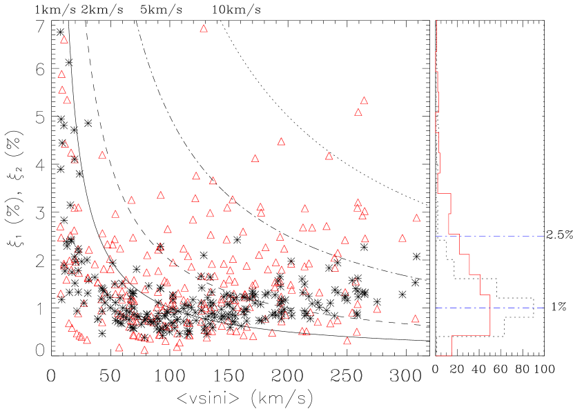
Figure 7: Left: Percentage error of the 251 measured stars. Asterisks: $\xi_{1}$ (%), individual region error indicator. Triangles: $\xi_{2}$ (%), measurements dispersion indicator. Lines represent constant values of $\xi$ in km s^-1. Solid: 1 km s^-1. Dashed: 2 km s^-1. Dot-dashed: 5 km s^-1. Dotted: 10 km s^-1. Right: Histogram of the percentage error. Solid line: $\xi_{1}$ (%). Dotted line: $\xi_{2}$ (%)

The number of regions used to determine $v\sin i$ depends on the quality of the spectra and the wavelength range, and is totally independent of $v\sin i$. The observational material analyzed here consist of 32 spectra in the range 4000–6000 Å in which we measured five regions, 116 spectra in the range 4000–5500 Å in which four regions were measured, 99 spectra in the range 3850–5000 Å or in the range 4000–5250 Å in which three regions were measured, and finally four objects in which only two regions were measured owing to excessive noise in part of the spectra.

Once $v\sin i$ and its error were obtained in all the regions of the same spectrum, the weighted mean value of $v\sin i$ was calculated, along with two different estimates of its uncertainty, $\xi_{1}$ and $\xi_{2}$, following the formulae proposed by González & Lapasset (2000, eq. 1) for radial velocities.

The error $\xi_{1}$ is the standard deviation of the weighted mean of a sample of $n$ uncorrelated observations with standard deviations $e_{i}$: $\xi_{1}=\left[\Sigma e_{i}^{-2}\right]^{-0.5}$. On the other hand, $\xi_{2}$ is a generalization of the standard error of the mean $\sigma/\sqrt{n}$ for a set of measurements weighted according to their individual errors. Therefore, $\xi_{2}$ is calculated from the dispersion of $v\sin i$ from different spectral regions, while $\xi_{1}$ is computed from the single measurement errors estimated through the calibration described in Sect. 3.4. In general, $\xi_{1}$ would be more appropriate when the number of measurements is small (2–3 spectral regions), and consequently the dispersion of measurements is a less precise estimate of the true error. In Figure 7 we have plotted the values of $\xi_{1}$ and $\xi_{2}$ computed for each object. Excluding slow rotators ($v\sin i$ below 30 km s^-1) whose line widths are close to the limit imposed by the spectral resolution ($c/R$ = 10–12 km s^-1), the error $\xi_{1}$ has an average value of 1.1%, always smaller than 2.5%. Regarding the dispersion of the values obtained from different regions of the same spectrum, only three objects with $\langle v\sin i\rangle>30$ km s^-1 were measured with $\xi_{2}$ over 5%, and the average error $\xi_{2}$ of these objects is 1.5%.

Figure 8: Position of the first zero of the FT of the rotational profiles for 8 spectral regions of 8 spectra of the star HD77370. Dotted lines are theoretical lines corresponding to different values of $v\sin i$ and have been calculated from the limb darkening coefficients in Díaz-Cordovés et al. (1995).

4.2 Application to late type stars

One field of application for the proposed method is the measurement of rotation in stars of spectral type F or later, where it is not possible to measure individual lines even for low rotators. As a test, we measured the rotational velocity of HD 77370, an F3 V star with projected rotational velocity of about 60 km s^-1, high enough for all spectral lines to appear blended. Eight high-resolution HARPS spectra of this star were downloaded from the ESO archive database. These spectra cover a spectral range 3800–6900 Å  with a S/N $\approx\,200$. Rotational velocities were measured for eight spectral regions of about 200–400 Å, using as template a synthetic spectrum with T_eff=6750 K and solar chemical abundances. Figure 8 shows the measured $v\sin i$ values for the eight spectra.

The dependence of the position of the first zero of the FT of the rotational profile with wavelength – due to the variation of the limb darkening coefficient with wavelength – is noticeable. The rotational velocity of each spectrum was calculated as the average of the eight spectral regions. The mean value of the 64 measurements is 59.16 km s^-1. The standard deviation of the measurements of the 8 spectra in one single spectral region is on average 0.41 km s^-1. If we take this value as the typical uncertainty of one of the 64 individual measurement, the uncertainty of the mean $v\sin i$ for each region should be $\sqrt{8}$ times lower (0.14 km s^-1). However, if we calculate the average for each of the eight spectral regions, then the dispersion of these mean rotational velocities is 0.37 km s^-1, indicating that the main source of uncertainty in these measurements is not random, but small systematic differences between the spectral regions. All in all, the uncertainty of the $v\sin i$ measured from a high-quality spectrum of an F-type star would be about 0.6%, demonstrating that high-precision rotational velocities can be measured even when lines are blended. The key point in this respect is the use of the template-template correlation function to model the subsidiary lobes of the object-template CCF during the calculation of the rotational profile. As an illustration, Figure 9 shows the reconstruction of the rotational profile for a small spectral region (70 Å) of the spectrum of HD 77370, where all spectral lines are blended.

Figure 9: Example of the rotational profile calculated from a high-S/N spectrum of only 70 Å for an F-type star. Upper panel: Object spectrum and template spectrum. Lower panel: the same as Fig. 1.

5 Discussion

To evaluate the performance of our method in determining $v\sin i$, we compared our results with those from Royer et al. (2002a). They used FT of line profiles to provide accurate $v\sin i$ of a large sample of A-type stars in the southern hemisphere observed with similar resolving power ($\sim$ 28000). Figure 10 shows Royer et al. values of $v\sin i$ and the ones obtained in this work for 155 objects in common with their sample. Even though a good agreement is found in stars of moderate, projected rotational velocities, a significant deviation is noticed for $v\sin i$ $>$ 150 km s^-1with an average difference of $5\pm 1$%, our values larger than theirs.

Figure 10: Comparison between our results and Royer et al. (2002a) for objects in common. Squares: normal stars. Circles: peculiar stars. Solid line: Normal stars fit $f({\rm\langle v\sin i\rangle})=1.43\;{\rm\langle v\sin i\rangle}^{0.92}$

There are several differences between the methodology used by Royer et al. (2002a) and the present work that can account for the effect present in Figure 10. First, they measured single lines in the range from 4200 Å to 4500 Å, i.e. a region of 300 Å wide which is the mean width of each region used in this work. Second, the blending effect becomes evident through the dependence of the number of measured lines with $v\sin i$. They used in average less than 3 lines on objects with $v\sin i$ $>$ 60 km s^-1, and over 90 km s^-1the average number of measured lines is $\leq 2$. Even though the dependence on the position of the first zero of the Fourier transform with the limb darkening coefficient was not taken into account by Royer et al., the adopted value $\varepsilon=0.6$ is typical of the limb darkening coefficient in the range of temperatures of the objects in the sample. However, an error of $\pm 0.01$ in $k_{1}$ represents an error of 1.5% in $v\sin i$. Thus, using a wrong $k$ value could account for 1.5% of the deviation detected in the comparison.

Finally, the main source of error is the uncertainty on the continuum position. Royer et al. (2002a) analyzed the magnitude of this effects by broadening synthetic spectra of $T_{\mathrm{eff}}$ from 7500 to 10000 K with $v\sin i$ = 10, 50, and 100 km s^-1. They found that in the coldest models with the largest $v\sin i$ the error can reach 3%. This uncertainty affects spectral lines giving as a result a lower value of $v\sin i$ than the real value. To evaluate the intensity of this type of systematic error with our method, we measured $v\sin i$ in a synthetic A5V spectrum broadened by $v\sin i$ = 20, 80, 120, 180, 220, and 280 km s^-1. Random noise was added to simulate S/N = 100, generating ten spectra with different noise pattern for each value of $v\sin i$. Then, four regions were used to measure $v\sin i$, and the average over the ten measures for each region was calculated. As expected, we found a tendency to measure a lower value of $v\sin i$ than the actual value. This effect is shown in Figure 11. Nevertheless, with the method proposed in this work the difference between measures and real values stays under 1% ($\langle\frac{v\sin i_{measured}}{v\sin i_{real}}\rangle_{150-300\;\rm km\,s^{-1}}=0.997\pm 0.004$) even for $v\sin i$ = 280 km s^-1. In conclusion, a considerable fraction of the difference between our results and those from Royer et al. (2002a) can be attributed to the effect of line blending on the continuum position. The influence of the line blending in high rotational velocity stars is significantly less with the proposed method than with Fourier transform of single-line profiles, by virtue of subtracting the secondary maximums from the CCF before calculating the Fourier transform. Similar results would be obtained by removing the blended lines with a similar procedure in the spectrum: modeling the smaller lines by convolving a rotational profile with a synthetic spectrum in which the line of interest has been subtracted.

Figure 11: Difference between real $v\sin i$ and average over ten consecutive measures with distinct random noise. Dotted line: $f({\rm\langle v\sin i\rangle})=0.0032\;{\rm\langle v\sin i\rangle}+0.0456$.

The main originality of the proposed method is the way in which the broadening function is built from the CCF, which, on the one hand, allows measurement of stars with blended spectral lines and, on the other, improves the S/N. Once the broadening function has been obtained, we determine the stellar rotation through the first zero of the FT. However, other alternative analyses are possible, such as direct fitting of the broadening function or Fourier-Bessel transformation (Piters, Groot, & van Paradijs 1996).

As an illustration, we used our method in combination with the Fourier-Bessel transformation to measure one of the objects in Piters et al. (1996) for which a HARPS spectrum was publicly available. These authors applied the Fourier-Bessel transformation method to individual spectral lines for measuring rotation in F-type stars. Owing to line blending, stars with $v\sin i>100$ km s^-1  could not be measured or had errors of about 10 – 20 %. We selected one of their fast rotating objects: HD 12311, for which they measured 110$\pm$22 km s^-1. We defined 5 spectral region between 3980 Å and 6530 Å  obtaining an average of 157.4 km s^-1with $\sigma=4.6$ km s^-1using our method with the FT first zero, and 155.9 km s^-1 with $\sigma=1.8$ km s^-1from our broadening function but using the Fourier-Bessel transform. Therefore, the application of Fourier-Bessel transform method to the broadening function derived from the CCF would be an excellent alternative for late-type fast-rotating stars. In the case of slowly rotating stars, however, the Fourier-Bessel transform is more sensitive to broadening effects that are different from rotation, so the zero of the FT would give better results (see sect. 3.1).

6 Summary

We have developed a method for measuring $v\sin i$ based on the FT of the central maximum of the CCF. This combination provides a simple and precise solution to the line blending problem with medium-resolution spectra and/or spectral types later than mid-A. As a result, the number of useful spectral regions per object with our method is independent of spectral type and $v\sin i$.

The high precision of the proposed method is supported by two key features of the procedure. The first one is to use an empirical calibration to take limb darkening effects into account in the position of the first zero of the FT, which is directly related to $v\sin i$. The second key feature is the subtraction of the subsidiary lobes of the CCF during the calculation of the rotational broadening function. This assures a good definition of the rotational profile even in presence of line blending.

The $v\sin i$ value is derived from the first zero of the FT of broadening function. However, the S/N of the resulting rotational profile is high enough to also do other detailed studies of the shape of the reconstructed rotational profile.

For slowly rotating stars, a lower limit for measurable $v\sin i$ is imposed by the instrumental profile and the intrinsic line width, which is included twice in our broadening function owing to the use of a template with lines of finite width. For metallic lines this limit is 5–8 km s^-1. In early-type stars the measurement is more difficult since metallic lines become weaker and He lines are usually not useful. Morphological differences between template and object are also less significant in late-type stars. For late-A type stars or later, differences in several subtypes have no impact on the rotation measurements.

We consider that, in accurate $v\sin i$ determinations, one significant contribution to the errors is the adopted value for the limb darkening. Even though in this work we use a wavelength-dependent coefficient, the continuum limb darkening might differ significantly from the line limb darkening. Using many spectral lines in our calculations, this difference might be averaged out, but systematic differences between lines and continuum might result in small but systematic $v\sin i$ errors. This is an issue that deserves further research.

We applied the proposed method to a sample of 251 A-type stars. Measurement errors are always under 2.5%, being 1.1% the average error for stars with $\langle v\sin i\rangle$ over 30 km s^-1. As regards the dispersion of values measured on different regions across a spectral range of $\sim 1150$ Å to $2000$ Å wide, we found standard errors of the mean below 5% with an average of 1.5%.

[x]crccc Results for 251 A1–A5 stars from the Bright Star Catalogue in the southern hemisphere.
HD $\langle vsini\rangle$ $\varepsilon_{1}$ $\varepsilon_{2}$ Spectral
$km\;s^{-1}$ $km\;s^{-1}$ $km\;s^{-1}$ Type
Continued.
HD $\langle vsini\rangle$ $\varepsilon_{1}$ $\varepsilon_{2}$ Spectral
$km\;s^{-1}$ $km\;s^{-1}$ $km\;s^{-1}$ Type

319 60.2 0.6 0.9 A1V
3719 53.4 0.8 1.3 A1m
4772 163.4 1.4 2.1 A3IV
6178 82.1 1.2 0.6 A2V
6767 151.3 1.9 0.8 A3IV
7804 115.1 1.0 1.3 A3V
9414 150.3 1.6 2.4 A2V
11753 14.7 0.9 0.01 A3V
14417 66.6 0.9 0.6 A3V
14943 115.0 0.5 0.8 A5V
15427 116.8 0.8 0.5 A2V
16754 167.6 2.0 1.7 A1Vb
17168 49.4 0.6 1.0 A1V
17254 126.5 2.1 0.9 A2V
17566 90.2 0.8 2.0 A2IV-V
17848 143.7 1.4 1.7 A2V
18331 264.8 3.4 8.0 A1Vn
18454 99.7 0.5 0.6 A5IV/V
18543 53.7 0.5 0.8 A2IV
18557 22.5 0.4 0.2 A2m
18623 102.5 1.3 1.2 A1V
20293 241.9 4.7 1.8 A5V
20888 79.3 0.6 0.6 A3V
21635 128.7 2.7 8.8 A1V
21882 265.2 3.5 6.5 A5V
21997 69.8 0.7 0.8 A3IV/V
22243 189.0 2.4 2.9 A2V
22634 68.9 0.9 1.7 A3V
23055 92.1 2.1 2.1 A3IV/V
23281 78.6 0.3 0.03 A5m
23738 193.3 3.2 4.8 A3V
24554 9.0 0.4 0.5 A2V
25371 135.7 1.2 0.7 A2V
27411 20.4 0.4 0.4 A3m…
27490 157.1 3.8 1.6 A3V
27861 194.3 2.3 8.7 A2V
28312 162.4 1.5 0.7 A3V
28763 102.7 1.2 1.3 A2/A3V
30127 193.3 2.1 3.0 A1V
30321 134.1 2.2 4.0 A2V
30422 127.0 1.8 1.2 A3IV
31093 196.8 1.9 4.4 A1Vn
31739 143.7 1.1 1.6 A2V
32667 144.0 1.2 0.9 A2IV
37306 148.1 1.9 3.6 A2V
38678 258.7 2.2 8.0 A2IV-Vn:
39421 254.3 4.0 2.3 A2Vn
39789 202.7 4.0 3.9 A3IV
41759 212.7 2.8 5.7 A1V
41841 58.2 0.4 0.5 A2V
42824 134.4 1.5 1.3 A2V
43319 73.7 0.6 0.3 A5IVs
43847 11.3 0.2 0.5 A2Vm…
43940 258.2 2.3 1.3 A2V
48915 16.7 0.4 0.3 A1V
50445 94.9 0.5 0.6 A3V
50747 84.3 0.6 0.7 A4IV
51055 42.8 0.2 0.3 A2V
53811 63.0 0.5 1.0 A4IV
55185 175.5 1.3 3.7 A2V
55595 154.9 1.1 2.4 A5IV-V
56405 145.7 1.8 2.8 A1V
57240 47.2 0.6 1.1 A1V
62864 71.9 1.3 0.5 A2V
65456 39.2 0.3 0.6 A2Vv
65810 239.3 2.0 4.9 A1V
66210 30.9 1.5 0.5 A2V
68862 91.9 0.5 1.0 A3V
69665 98.2 0.9 2.6 A1V
70340 10.6 0.3 0.2 A2Vpn:EuSrCr:Si
70612 104.1 0.6 0.7 A3V
71267 19.8 0.3 0.4 A3m
71688 132.1 1.6 0.7 A1/A2V
71815 39.1 0.3 0.6 A1/A2V
72660 8.1 0.4 0.2 A1V
72968 15.9 0.5 0.4 A1pSrCrEu
73997 193.7 2.8 2.2 A1Vn
74190 59.4 0.4 0.7 A5m
74341 97.6 0.9 1.5 A3V
74879 63.5 0.6 0.8 A3IV/V
75171 96.5 0.6 0.6 A4V
75630 163.7 1.6 2.1 A2/A3IV
75737 16.5 0.4 0.7 A4m
75926 194.5 2.2 1.4 A1Vn
76483 68.9 0.4 0.5 A3IV
78045 30.6 0.4 0.5 kA3hA5mA5v
78676 56.1 0.4 0.5 A4IV
78922 108.3 0.5 0.3 A4IV-V
79193 10.4 0.5 0.2 A3III:m+A0V:
80007 145.7 1.2 2.2 A2IV
80447 15.1 0.2 0.3 A2Vs
80951 23.7 0.9 0.1 A1V
81157 36.6 0.6 0.7 A3IVs…
81309 10.6 0.2 0.7 A2m
82068 258.9 3.5 2.8 A3Vn
82446 54.0 0.6 1.6 A3V
83520 149.6 1.3 1.8 A2,5V
83523 134.4 0.9 1.8 A2V
85558 134.6 1.4 3.4 A2V
86266 186.6 1.6 0.9 A4V
86301 218.9 1.7 2.0 A4V
88024 92.3 1.3 3.1 A2V
88372 259.2 4.2 8.3 A2Vn
88522 23.1 0.5 0.4 A1V
88842 78.9 0.6 0.3 A3IV-V
88955 103.6 0.9 1.1 A2Va
89263 67.2 0.8 0.5 A5V
89816 214.3 2.0 6.6 A4IV/V
90630 90.9 0.7 0.4 A2,5V
90874 65.7 0.5 0.4 A2V
91790 111.7 0.8 1.3 A5IV/V
93397 94.0 0.4 0.9 A3V
93742 49.8 0.5 0.9 A2IV
93903 19.4 0.4 0.6 A3m
93905 118.3 1.2 2.2 A1V
94985 181.0 1.4 4.1 A4V
95370 111.6 1.1 2.5 A3IV
96124 156.3 1.9 0.8 A1V
96146 7.7 0.3 0.03 A2V
96441 130.3 1.0 1.3 A1V
96723 25.4 0.5 0.1 A1V
103101 42.1 0.5 0.4 A2V
103266 165.1 1.6 1.0 A2V
104039 12.6 0.3 0.2 A1IV/V
105776 153.1 1.1 5.0 A5V
105850 126.8 1.2 1.4 A1V
106819 79.0 0.6 1.1 A2V
107070 202.3 1.9 3.0 A5Vn
108107 242.1 3.2 5.2 A1V
108925 188.9 1.7 2.7 A3V
109074 89.9 0.6 1.2 A3V
109704 155.4 1.3 1.8 A3V
109787 296.8 3.8 7.3 A2V
111588 60.6 0.5 0.5 A5V
114330 7.4 0.5 0.2 A1IVs+…
114576 162.0 2.0 4.2 A5V
115892 90.3 1.0 1.6 kA15hA3mA3va
116061 194.2 1.5 2.4 A2/A3V
116197 239.7 3.3 4.4 A4V
117150 220.4 2.4 5.9 A1V
117558 169.8 2.2 2.1 A1V
118098 232.6 2.2 6.3 A3V
119938 69.7 0.4 0.3 A3m…
122958 172.2 1.9 7.1 A1/A2V
123998 17.2 0.3 0.1 A2m
124576 126.5 1.4 2.1 A1V
125283 257.3 3.6 4.0 A2Vn
126367 65.8 0.6 0.7 A1/A2V
126722 101.2 0.7 1.1 A2IV
127716 96.4 0.8 0.3 A2IV
130841 59.6 0.9 0.8 kA2hA5mA4Iv-v
132219 42.9 0.4 1.8 A4V+,,,
133112 96.4 0.6 1.0 A5m
134482 160.4 1.0 1.5 A3IV
134967 259.4 3.2 13.2 A2V
135235 75.9 0.5 0.3 A3m
135379 68.5 0.9 0.8 A3Va
137015 119.6 1.4 3.4 A2V
137333 44.1 0.6 0.8 A2V
138413 21.4 0.2 0.1 A2IV
138965 102.7 1.0 2.0 A1V
141413 116.6 0.6 0.8 A5IV
142139 89.2 0.7 0.7 A3V
142445 137.7 1.1 1.4 A3V
142629 43.0 0.6 1.1 A3V
143101 86.1 0.6 0.6 A5V
145570 42.3 0.6 0.5 A3IV
145607 217.7 2.7 4.2 A4V
145689 106.4 0.8 0.5 A4V
146667 225.2 2.5 1.6 A3Vn
148367 19.5 0.8 0.8 A3m
150573 235.8 2.6 1.6 A4V
150894 136.2 0.8 0.9 A3IV
151676 149.4 1.2 1.1 A3V
152127 31.6 0.5 0.7 A2Vs
153053 102.8 0.7 1.0 A5IV-V
154310 263.0 3.5 7.7 A2IV
154418 72.6 0.6 0.6 A1m,,,
154494 114.8 0.6 0.8 A4IV
154895 121.6 1.1 4.0 A1V+F3V
155259 214.0 3.2 4.0 A1V
159492 54.1 0.4 0.7 A5IV-V
160613 112.6 1.2 1.6 A2Va
164577 194.6 1.8 3.5 A2Vn
165189 129.8 0.8 0.7 A5V
165190 129.2 0.7 1.4 A5V
166393 191.7 3.0 3.0 A2V
166960 27.3 0.3 0.3 A2m
167564 153.0 1.3 1.8 A4V
169853 22.6 0.3 0.7 A2m
170384 131.3 0.6 0.5 A3V
170479 67.6 0.7 2.2 A5V
170642 177.3 1.3 5.3 A3Vn
171856 106.1 0.8 0.2 A5IV
172555 116.4 0.6 0.5 A7V
172777 148.6 1.6 4.6 A2Vn
173715 122.3 0.9 4.6 A3V
175638 151.1 0.9 2.7 A5V
175639 214.3 1.8 2.9 A5Vn
176687 68.9 0.4 0.3 A2,5Va
176984 30.0 0.6 0.1 A1V
178253 203.2 1.7 2.8 A2Va
180482 80.4 0.7 1.4 A3IV
181383 180.7 2.3 1.4 A2V
183545 226.5 2.3 3.0 A2V
184552 13.1 0.3 0.7 A1m
184586 197.7 2.3 1.7 A1V
187421 170.0 2.3 2.5 A2V
187653 248.2 3.0 6.0 A4V
188899 69.7 0.6 1.1 A2V
189118 45.2 0.5 0.6 A4/A5IV
189388 248.4 3.1 3.3 A2,5V
189741 137.9 1.2 2.3 A1IV
197725 153.4 1.5 3.1 A1V
198001 115.4 1.2 2.4 A1,5V
198160 183.0 2.4 3.3 A2,5IV-V
198161 176.7 1.9 5.5 A2,5IV-V
198529 275.4 3.1 2.7 A2Vn
198743 51.7 1.0 1.2 A3m
199475 212.0 3.4 1.1 A2V
201906 264.4 6.0 14.1 A1V
202730 135.6 1.8 2.6 A5Vn:
203562 58.0 0.7 1.3 A3V
204394 132.7 1.1 2.2 A1V
204854 107.1 1.0 1.4 A2IVv
205765 172.2 2.2 2.6 A2V
205811 102.6 1.3 1.3 A2V
207155 136.6 1.5 5.0 A2V
208321 215.6 1.9 1.1 A2Vn
208565 308.8 6.4 8.9 A2Vnn
210049 307.7 4.7 2.4 A1,5IVn
210739 189.7 1.6 3.7 A3V
212728 250.1 2.9 0.8 A4V
213884 165.0 1.2 3.1 A5V
214085 163.4 2.0 2.0 A3Vn
214150 80.9 0.7 1.7 A1V
214484 8.5 0.1 0.5 A2Vp
215729 170.5 2.1 0.7 A2V
216627 83.2 0.6 0.3 A3V
216900 67.0 0.4 0.8 A3Vs
216956 91.6 0.5 0.4 A4V
217498 91.9 1.3 2.1 A2V
218108 194.5 1.7 1.9 A3,5V
219402 154.2 1.8 2.0 A3V
221675 57.2 0.5 0.1 A2m
221760 22.4 0.5 0.5 A2VpSrCrEu
222602 234.7 4.3 9.8 A3Vn
223438 89.0 0.5 0.9 A5m
223466 69.5 0.9 0.6 A3V
223991 19.1 0.9 0.5 A2V+F2V
224361 95.6 0.8 1.5 A1IV