A statistical study of the luminosity gap in galaxy groups

Abstract

The luminosity gap between the two brightest members of galaxy groups and clusters is thought to offer a strong test for the models of galaxy formation and evolution. This study focuses on the statistics of the luminosity gap in galaxy groups, in particular fossil groups, e.g. large luminosity gap, in an analogy with the same in a cosmological simulation. We use spectroscopic legacy data of seventh data release (DR7) of SDSS, to extract a volume limited sample of galaxy groups utilizing modified friends-of-friends (mFoF) algorithm. Attention is paid to galaxy groups with the brightest group galaxy (BGG) more luminous than $M_{r}$= -22. An initial sample of 620 groups in which 109 optical fossil groups, where the luminosity gap exceeds 2 magnitude, were identified. We compare the statistics of the luminosity gap in galaxy groups at low mass range from the SDSS with the same in the Millennium simulations where galaxies are modeled semi-analytically. We show that the BGGs residing in galaxy groups with large luminosity gap, i.e. fossil groups, are on average brighter and live in lower mass halos with respect to their counter parts in non-fossil systems. Although low mass galaxy groups are thought to have recently formed, we show that in galaxy groups with 15 galaxies brighter than $M_{r}\geq-19.5$, evolutionary process are most likely to be responsible for the large luminosity gap. We also examine a new probe of finding fossil group, $\Delta m_{14}\geq 2.5$, and find that the fossil group selected according to new probe are more abundant than those selected using the conventional probe, $\Delta m_{12}\geq 2$, in low halo mass regime, $\leq 10^{14}M_{\odot}$ . In addition we extend the recently introduced observational probe based on the luminosity gap, the butterfly diagram, to galaxy groups and study the probe as a function of halo mass. This probe can, in conjunction with the luminosity function, help to fine tune the semi-analytic models of galaxies employed in the cosmological simulations.

1. Introduction

Galaxy groups are key systems in advancing our understanding of structure formation and evolution in the universe as, in a hierarchical framework, they span the regime between individual galaxies and massive clusters. Advances in the cold dark matter cosmological simulations and improvements on the particle mass resolution has provided the opportunity to study galaxy groups or low mass halos. The Millennium simulation (Springel et al., 2005) is a recent example. The semi-analytic models of galaxy formation are also employed to understand the formation and evolution of galaxies in cosmological context.

The key factor in the success of this attempt is the availability of observational constraints to help fine tune the models. While galaxy luminosity function has been widely used as a strong constraint, the number of physical processes and the free parameters in the models limits the achievements.

There is a class of galaxy groups, dubbed as fossil groups (Ponman et al., 1994), which are the archetypal relaxed systems and arguably the end product of the galaxy mergers within the group. The selection criteria for fossils is outlined by Jones et al. (2003), i.e. groups with an X-ray luminosity of $L_{x,bol}\geq 0.25\times 10^{42}$ h^-2ergs^-1, and a minimum luminosity difference of 2 magnitude between the first- and second-ranked galaxies ($\Delta M_{12}\geq 2$), within half the projected $R_{200}$ radius, where $R_{200}$ is the radius within which the mean density is 200 times the critical density of the Universe.

Implementation of cosmological simulations in which the evolution of the halos can be traced, has given strong evidences that fossil groups, or galaxy systems with large luminosity gap $\Delta M_{12}$, on average form earlier than galaxy groups with small luminosity gap (Dariush et al. 2007, 2010). The early formation epoch for fossil groups had been argued previously based on observations of about a dozen such systems. They included the study of X-ray scaling relations (Khosroshahi et al., 2007) as well as the morphological studies of the brightest group galaxies (BGGs) in fossil groups (Khosroshahi, Ponman & Jones, 2006).

A statistical comparison between the properties of observed fossil groups and those in the cosmological simulations requires dozens of such systems to be identified observationally which is currently unavailable due to the nature of existing X-ray surveys (often shallow or very limited in angular coverage). Santos et al. (2007) have cross-correlated optical and the Sloan Digital Sky Survey (SDSS) and the ROSAT All Sky Survey (RASS) (Voges et al. 1999) and identified 34 fossil group candidates covering a wide range of redshift. The applied methodology, however, does not produce a complete sample of fossil groups.

Although conventionally an X-ray threshold has been applied to the IGM in fossil groups a lot can be learned from the selection based on optical criterion alone, e.g. “optical fossils” (Dariush et al., 2007). Identifying low-mass fossil systems is hampered by the fact that groups are under-represented in existing X-ray catalogs, however, based on simulation data Dariush et al. (2007) have shown that even applying X-ray criteria, the fraction of late-formed systems that are spuriously identified as fossils is $\sim 4-8$ per cent, almost independent of halo mass.

The main driver of this study is to find out the extend at which the luminosity gap in low mass groups can shed light on the formation of these systems and quantify the observed properties related to the luminosity gap which can be compared with semi-analytic models. As the large luminosity gap between the galaxies in a galaxy group can have a statistical origin, it would be therefore useful to find out to what extend the large luminosity gap is a representative of the evolutionary processes as opposed to have been originated statistically. Furthermore we provide observational measures which can be used to constrain the semi-analytic models of galaxy formation.

The paper is organized as follows; Section 2 describes the databases and the simulations. Algorithm used to extract the sample of groups in observation is described in section 3. Biases and completeness of the sample is discussed in section 4. In section 5 we present the derived group properties. Selection criteria for identifying fossil group is discussed in section 6. Results are presented and discussed in sections 7 to 9 with concluding remarks presented in section 10.

For this study we assume, $h=0.7$, $\Omega_{m}=0.3$, and $\Omega_{\Lambda}=0.7$.

2. Data

2.1. Observation

We use the legacy archive of the latest data release of the SDSS, DR7 (Abazajian et al., 2009) which covers 8,423 square degrees in imaging data (which contains roughly 360 million distinct photometric objects) and the spectroscopic survey mapped 8032 square degrees (1,640,000 objects with measured spectra). We confine the study to those objects identified in SDSS as galaxies. In this study, we use both the photometric and the spectroscopic data.

Initially we restrict the study to galaxies within the redshift range of $0.02<z<0.17$, retaining only those with clean spectra (flag=0) providing us with a sample of 601,981 galaxies. The lower limit on the redshift is dictated recalling that, objects with $z<0.02$ are often stars and the upper limit on redshift is placed in order to confine the study to the range where the spectroscopic sample is complete. It worths stressing that, the main galaxy spectroscopic sample of SDSS is restricted to Petrosian magnitude, $r_{petro}<17.77$.

We extract objects with $r_{petro}<21.0$, identified as galaxy, from the photometric sample of SDSS DR7. For galaxies fainter than $r_{petro}=21.0$, the error in apparent magnitude increases rapidly (Oyaizu et al. 2008). For objects satisfying the above conditions, we retrieved the Petrosian magnitudes (Petrosian 1976; Strauss et al. 2002) and K-corrected them using the method described in Blanton et al. (2003a).

2.2. Simulation

In this paper we use the galaxy group catalog from the Millennium simulation (Springel et al., 2005) and the associated semi-analytic model of galaxy formation by Bower et al. (2006). Below we briefly describe these simulations.

The Millennium simulation utilizes a $\Lambda CDM$ cosmological model to follow structure formation from $z=127$ up to the present epoch. Starting with an inflationary, dark-matter dominated universe, structures form through the bottom-up hierarchy, i.e., starting with small scale density fluctuations resulting in large scale structures we observe today. Evolution of $2160^{3}$ particles each with $8.6\times 10^{8}h^{-1}M_{\odot}$ has been followed from $z=127$ up to present day ($64$ time-slices of positions and velocities were stored, separated logarithmically between $z=127$ and $z=0$) through a comoving box of $500Mpc$ on each side, (Springel et al., 2005) with $\Omega_{\Lambda}=0.75$, $\Omega_{M}=0.25$, $\Omega_{b}=0.045$, $h=0.73$, $n=1$ and $\sigma_{8}=0.9$ based on WMAP observations, (Spergel et al., 2003) and 2dF galaxy redshift survey, (Colless et al., 2001). The evolution of a structure has been followed only if it composed of at least, 20 particles (equivalent mass is $1.72\times 10^{10}h^{-1}M_{\odot}$) at that epoch (Springel et al., 2005). In addition, friends-of-friends algorithm was exploited to extract haloes with densities at least $200$ times the critical density and substructures were identified using SUBFIND algorithm developed by Springel et al. (2001).

The underlying dark matter haloes of the Millennium simulation was used to simulate the growth of galaxies, by self-consistently implementing a semi-analytic model of galaxies on the outputs of the Millennium simulation (Bower et al., 2006). This semi-analytic model accounts for the feedback from supernova explosions as well as AGNs in modeling the massive halos. In addition, AGN feedback has been considered as an operation which quenches the star-formation and star-bursts are triggered both by merging and disk-instabilities. Bower et al. (2006) predicts the luminosity function of galaxies in B and K band for the present epoch as well as the present day color distribution. For the purpose of this study, we use the catalogue of Bower et al. (2006) semi-analytic model and retrieved the absolute r-band magnitude for group members, the halo mass of the group as well as the mass of the subhalo containing the BGG at the present epoch.

2.3. Monte Carlo Simulation

The idea behind performing the Monte-Carlo simulation is that the luminosity gap between the two brightest members (or between any other members) of a galaxy system can also have a statistical origin.

We expect large luminosity gaps to appear preferentially in groups with few members. In order to understand the extend at which the luminosity gap with statistical origin affects our analysis and results, we perform a Monte-Carlo simulation by drawing random samples from an underlying Schechter function (Schechter 1976).

We generate a sample of $\sim 10^{6}$ galaxy groups with different number of members within the completeness of the observed sample described in section 4. We choose the underlying luminosity function to have Schechter parameters of $\alpha=-1.08$ and $M_{r}^{*}=-21.62$ as in Zandivarez et al. (2006), with galaxy luminosity ranging from $M_{r}=-16$ to $-26$. The chosen values are the best fit Luminosity function for groups based on the r-band SDSS data.

3. Selecting groups in observational data

3.1. The Algorithm

To identify galaxy groups, we use the modified friends-of-friends (mFoF) algorithm developed by Paredes et al. (1995) which is a modification of FoF (Huchra & Geller, 1982), one of the most frequently applied methods for finding structures in redshift surveys. The starting point in this algorithm is that every galaxy can be the center of a group of galaxies. The algorithm, however, will gradually lead to the most probable center, for a given search radius.

Given this, we start by looking for companions of each galaxy within a specified search physical radius, $r_{s}$. A galaxy is companion to the chosen galaxy if it falls within the search radius in the plane of the sky and within the redshift interval of $\Delta z$. For this study we choose $r_{s}$ to be the equivalent of 500 kpc at the redshift of the galaxy in the spectroscopic sample and $\Delta z$=0.002.

For the first generation of the groups, we count the number of companions with the above constraints for each galaxy in the spectroscopic sample described in section 2.1. Naturally most of the members will be shared by galaxy groups found in the first generation. Comparing overlapping groups, those with fewer number of member will be removed from the list if they fall within the $r_{s}$ measured from the center of the richer group and $\Delta z$=0.002. This results in the second generation of the galaxy groups. Having this, we calculate the mean redshift and luminosity weighted center of each of the surviving groups and the process of removing the small groups overlapping with larger groups continues until there is no common members between any two groups of galaxies.

As it was described, mFoF works with two free parameters,$r_{s}$ and $\Delta z$, and their values are set depending on the science goals of the study, e.g. Miller et al. (2005) and von der Linden et al. (2007) have been used $r_{s}=1Mpc$ ; $\Delta z$=0.002 and $r_{s}=2Mpc$ ; $\Delta z$=0.01 to identify cluster of galaxies, respectively. Also, Einasto et al. (2005) adopted $r_{s}=0.5Mpc$ ; $\Delta z$=0.002 to make catalogue of group/cluster. Here we aim at studying galaxy groups and low mass haloes for which we find our choice suitable in comparison to the existing galaxy group catalogs. We extracted 81614 and 6956 groups with more than 2 and 5 spectroscopic members $(richness)$, respectively.

There exist several catalogues of groups and clusters of galaxies extracted from the SDSS data: Catalogues by Goto (2005, DR2), Miller et al. (2005, DR2), Merchan and Zandivarez (2005, DR3), Berlind et al.(2006, DR3), Zandivarez et al. (2006, DR4), Yoon et al. (2008, DR5) and Tago et al. (2008, DR5). In each of the above mentioned catalogs, criteria implemented through the group-finder algorithm has been chosen on the basis of the type of the corresponding study. To check if our extracted groups, based on conditions adopted here, overlap with those from previous studies, we performed a cross-matching between our extracted catalog and two other popular group samples in the literature: the Abell cluster (Abell 1958) and C4 (Miller et al. 2005) catalogs. It worth stressing that although C4 is known as a “galaxy cluster catalog”, it has a wide mass range making it suitable for the comparison with our “galaxy group” catalog.

For the redshift of Abell clusters we used published data by Struble et al. (1987) in which there are 838 with determined redshifts out of 2712 Abell clusters. There are 318 Abell clusters that lie in the area of sky coverage for the SDSS DR7 and have redshifts in the range of $0.02<z<0.17$. For our groups of richness $\geq 5$ (spectroscopic members), 195 out of 318 Abell clusters $(61\%)$ are matched within $10^{\prime\prime}$ of our group center. In addition, we selected the groups of richness $\geq 2$ and in this case, 283 out of 318 Abell clusters are matched ($88\%$). The C4 catalog was generated using a cluster finding algorithm which identifies clusters as over densities in a seven dimensional space of position and colors (Miller et al. 2005). The catalog contains 748 clusters with richness more than 10 members brighter than r = 17.7. Applying the above search criteria we found 549 of 748 C4 clusters, $73\%$ within $0.02<z<0.17$. Reducing the number of galaxies per group, $\geq 2$, we would find $96\%$ of C4 clusters, which shows a very large overlap between our extracted groups and the C4 catalog.

Figure 1.— Color-magnitude relation for members residing within a centered at the BGG position with a radius of 0.5 Mpc at the BGG redshift. The 2$\sigma$ boarders and restrictions on apparent magnitude are also illustrated.

3.2. Color-Magnitude Relation

As noted earlier, the main spectroscopic sample of the SDSS is complete to the Petrosian $r<17.77$. However, the photometric sample reaches lower luminosities. Moreover, the tiling algorithm used in SDSS spectroscopic survey (Blanton et al., 2003b), leaves some galaxies unobserved spectroscopically because of fiber collisions. Yoon et al. (2008) estimated the spectroscopic completeness of the SDSS DR5 to be $f_{spec}\sim 65\%$ for rich clusters. In order to have a realistic estimate of the optical luminosity and the richness of the extracted groups we use the color magnitude relation (hereafter CMR) to identify additional group member candidates. Observational evidences have shown that the bulk of the early-type galaxies in clusters and groups lie along a linear CMR. This relation is shown to have a small scatter (e.g., Bower et al. 1992; Peebles et al. 2002; Kodama et al. 1998) and can be used as a robust method for finding galaxy systems (e.g., Gladders et al. 2000). Although there are uncertainties in the CMR method of group membership identification, we use the photometric members only to estimate the global properties, such as the number of galaxies per groups and the total luminosity of the group.

In order to incorporate the photometric data into the analysis, we consider all the photometric and spectroscopic galaxies within an angular distance equivalent to 500 kpc around the group center if they fall on the CMR. It should be noted that, group center is defined as the brightest member of the group. For this purpose, we fit a line to the color-magnitude diagram of the spectroscopic members if the group has at least three members with $M_{r}\leq-19.0$. We determine the slope and intercept of the CMR for each group. We consider only those photometric ($m_{r}\leq 21$) and spectroscopic galaxies which fall within $\pm 2\sigma$ of the color magnitude relation defined by spectroscopic members. An example of a fitted CMR to color magnitude diagram for one of our groups is shown in Fig. 1.

Member selection using the color-magnitude relation method is hampered by miss-identification of forground and background galaxies as group members. In principle, miss-identification of members will affect the total luminosity and in turn the estimated mass (§5.2). In order to quantify the uncertainty in halo mass estimate we randomly selected field regions in the SDSS. We chose galaxies within a radius comparable to that of groups in each field region and applied color-magnitude selection. The contribution of the field galaxies on the halo mass of groups was found to be negligible.

We assume all the photometric group members found using the CMR to have the mean redshift of the group defined by the spectroscopic members.

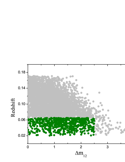
Figure 2.— 4113 groups with $M_{r,BGG}\leq-22$ are shown in redshift vs. $\Delta m_{12}$ diagram. The green rectangle area represents the selected region which is free of biases.

4. Bias Correction and Completeness

As noted in §2.1, we have used the main spectroscopic sample and photometric legacy survey of SDSS DR7 as our spectroscopic and photometric input. Statistical properties of the input data is discussed here along with the constrains resulted from the completeness and bias removal from the samples. For the photometric sample, Abazajian et al. (2009) demonstrated that the sample is $95\%$ (95% completeness limit for point sources) complete to $r\approx 22.2$. Whereas, the main spectroscopic sample of SDSS DR7 is complete to a r-band petrosian magnitude (Petrosian, 1976) of $r\simeq 17.77$, corrected for Galactic extinction (Schlegel et al. 1998; Strauss et al. 2002; Abazajian et al. 2009).

The limiting magnitude of $r\simeq 17.77$ is equal to $M_{r}\simeq-17$ at $z=0.02$ and $M_{r}\simeq-21.8$ at $z=0.17$. As we are interested in large luminosity gap, i.e. $\Delta m_{12}\geq 2$ magnitude, the above completeness limit will naturally bias our analysis toward low luminosity gap at higher end of the redshift distribution. This is shown in Fig.2.

To overcome this, we apply the $M_{r}$$\leq-22$ constraint to the BGGs both in the observed SDSS groups (4113 groups) and in the simulations (18843 groups). The constrain on the BGG luminosity is also consistent with the value adapted for the $M^{*}$ parameter in Schechter luminosity function in r-band. In addition this selection helps to compensate the absence of X-ray data, given the correlation of the BGG luminosity with the IGM X-ray emission (Khosroshahi et al., 2007; Ellis & O’Sullivan, 2006), and thus reduces contamination from individual galaxies that are not associated with a group scale halo.

To ensure that a luminosity gap up to 2.5 mag can be observed without a bias, the second brightest galaxy should be at least as luminous as -19.5 mag which corresponds to the limiting apparent magnitude of the spectroscopic sample, i.e $r\simeq 17.77$ mag at $z=0.065$. In other words, our luminosity gap estimates less than 2.5 magnitude should be bias free for groups within $0.02\leq z\leq 0.065$. We therefore restrict the observed galaxy sample to the above redshift range.

Applying the above mentioned restrictions ($\Delta m_{12}$$\leq 2.5$ and $z\leq 0.065$) resulted in 109 fossils out of 620 groups (see. §6).

5. Estimating Physical Parameters for Groups

Based on available parameters for members of each galaxy group, we have derived a number of quantities both for simulated and observed groups which is discussed here.

5.1. Velocity Dispersion and Virial Radius

According to Beers et al. (1990), a reliable method for measuring the velocity dispersion in groups with few members is the so-called gapper estimator (e.g. Yang et al. 2005). Since our groups catalogue contains low member groups we use this method to estimate the line-of-sight velocity dispersion of each individual group.

The method involves ordering the set of recession velocities ${v_{i}}$ of the $N$ group members and defining gaps as

$$g_{i}=v_{i+1}-v_{i},\quad\quad i=1,2,...,N-1.$$ (1)

The rest-frame velocity dispersion of our groups is then given by

$$\sigma_{gap}=\frac{\sqrt{\pi}}{(1+z_{group})N(N-1)}\sum_{i=1}^{N-1}{w_{i}g_{i}}.$$ (2)

where the weight is defined as $w_{i}=i(N-i)$ . As the central galaxy in each group, is assumed to be at rest with respect to the dark matter halo, the estimated velocity dispersion has to be corrected by a factor of $\sqrt{N/(N-1)}$ (Yang et al., 2005). This results in a final velocity dispersion given by

$$\sigma_{v}=\sqrt{\frac{N}{N-1}}\sigma_{gap}.$$ (3)

As we will see in the next section, an estimation of the virial radius of the galaxy groups is also required. Using the Virial theorem, Girardi et al. (1998) derives an approximation for the virial radius of a spherical system as:

$$R_{vir}=\frac{\sqrt{3}}{10}\frac{\sigma_{v}}{H_{0}}\quad Mpc$$ (4)

where $\sigma_{v}$ is the velocity dispersion of group members.

On the other hand, for the simulated groups, given that the halo mass is derived directly by adding the mass of the dark matter particles, $R_{vir}$ is calculated as follows:

$$R_{vir}=\frac{GM_{halo}}{\sigma_{v}^{2}}\quad Mpc$$ (5)

where $M_{halo}$ is the total mass of the halo and $\sigma_{v}$ denotes the velocity dispersion of group members.

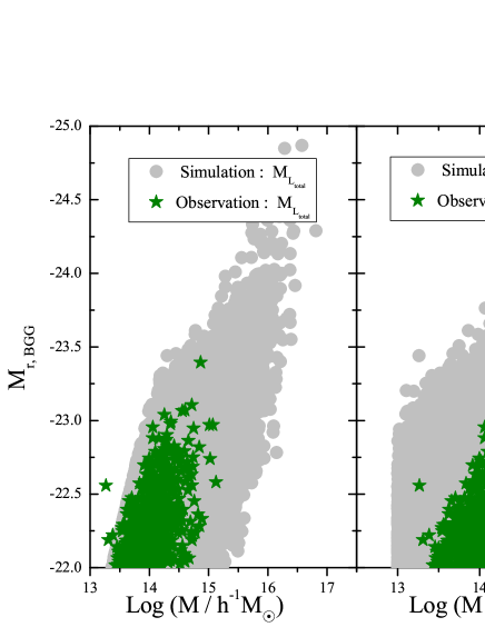
Figure 3.— The distribution of the galaxy groups in the plane of total mass of the group and the BGG luminoisty. Total mass of the simulated groups are estimated based on total luminosity Eq 6 (left) and dark matter particles (right). The mass of observed groups are based on the total luminosity. It is noticeable that, total mass obtained through total luminosity is in a better agreement with the observations.

5.2. Halo Mass

For observed groups, the total luminosity was used as diagnostic of halo mass, as appeared to be a better mass estimator than the line-of-sight velocity dispersion (Popesso et al. 2005; Miller et al. 2005; Lin et al. 2004) :

$$log(h^{-1}M)\approx-2.46+1.45log(h^{-2}L_{r})$$ (6)

where $L_{r}$ is the total r-band luminosity of the galaxy group, defined as the sum of the r-band luminosity of member galaxies with $M_{r}<-19.5$, (Milosavljevic et al. 2006).

In addition to the measurement of $M_{halo}$ in the simulated groups, we also estimate the halo mass using the empirical relation (Eq. 6) for consistency. In Fig. 3, the two methods of mass estimation are compared. Left panel compares the distribution of the halos in the plane of total gravitational mass based on Eq. 6 and the luminosity of the BGG for both the simulated and the observed systems. The same is shown in the right panel with the mass of the simulated halos obtained from the dark matter only. As expected, a better consistency is achieved when the luminosity based estimation is applied to the observations and the simulations. Therefore this mass indicator is used in the our analysis to avoid any systematics. The same method was applied in assigning a mass to the halos in the Monte Carlo simulations (see. §2.3).

Figure 4.— The normalized histogram of number of galaxies per group is compared between simulated and observed groups. The K-S test shows that the probability of two samples selected from a common distribution is $\sim$ $10^{-21}$.

5.3. Richness

To obtain the number of galaxies per group we applied $M_{r}\leq-19.5$ criterion to the observed and the simulated groups (Millennium and Monte-carlo). The distribution of richness for the observed and the simulated groups is shown in Fig. 4. This plot illustrates that, richness of simulated and observed groups are different which might be related to different group selection procedures in simulation and observation data. The group selection in simulations is based on a full knowledge of the three dimension distribution of dark matter subhalos (e.g. galaxies), while as noted earlier, the group selection in observations is based on two dimension distribution of galaxies complemented by slices the redshift space. However, the difference in shape of the distributions has no impact on our conclusions.

In order to study the impact of biases on statistics of number of galaxies per group, generated groups through the Monte Carlo simulation had to span a large range of richnesses ($10^{4}$ simulations were carried out for each richness class of group).

6. Selection of Fossil Groups

In low-density environments, the merging of compact groups can lead to the formation of the fossil groups (Vikhlinin et al. 1999; Jones et al. 2003). These class of systems have masses which are comparable to those of normal groups and clusters of galaxies. Observationally, the identification of fossils have so far been based on the definition of fossil group suggested by Jones et al. (2003). In Jones et al. (2003) definition, a fossil group has an X-ray luminosity of $L_{X,bol}\geq 0.25$ $\times$ $10^{42}$ $h^{-2}$ $erg$ $s^{-1}$, and the dominant galaxy is at least 2 magnitudes brighter (in r-band) than the second ranked galaxy within $0.5R_{200}$ of the group. Assuming a circular orbit, the $L^{\ast}$ galaxies merge with the central galaxy within a few Gyr due to orbital decay as a result of the dynamical friction (Jones et al. 2003).

The existing X-ray surveys overlapping the area covered by the SDSS survey are either wide and shallow (ROSAT All Sky Survey, Voges et al. 1999) or very small and deep. As a result, facing the lack of suitable X-ray data we limit the study to optical fossils or galaxy groups with a large luminosity gap (Dariush et al. 2007). The X-ray criterion is conventionally used to ensure that only group-mass halos have been selected. As noted earlier we compensate this by the introduction of lower limit in the BGG luminosity.

The luminosity gap was measured within half a virial radius, $R_{vir}$, derived using equations 4 and 5. This is slightly different to the definition of the Jones et al. (2003), however the difference applies to both the simulations and observations, consistently.

Similar to observational constrains discussed in §4 ,the same conditions was applied to simulation data to select optical fossil groups with the exception of the X-ray luminosity criterion. Also following Dariush et al. (2007), we limit the analysis to groups with $log(M_{halo}/h^{-1}M_{\odot})>13$.

These conditions resulted in 1993 fossil systems out of 16688 groups, or roughly $12\%$. Furthermore, fossil groups through the Monte Carlo simulation, were defined as groups $\Delta m_{12}\geq 2$ and $M_{r,BGG}\leq-22$ in accordance with definitions for observation and simulation data.

In order to compare the properties of fossil with non-fossil groups, we introduced control groups with $\Delta m_{12}\leq 0.5$ and satisfying the remaining conditions mentioned above (e.g. $M_{r,BGG}\leq-22$), in observations and simulations. This provides us with 85 and 2419 control groups in observed and simulated catalogs, respectively.

Figure 5.— The distribution of r-band absolute magnitude of fossil BGGs is compared to the same in control groups for observational and simulation samples. Fossil BGGs are brighter than control BGGs. The K-S test shows that the probability of control and fossil samples being drawn from similar distribution are $1.2\times 10^{-3}$ and $3.6\times 10^{-64}$ in observation and simulation samples, respectively.

Figure 6.— The distribution of BGG absolute magnitude over group halo mass is compared between fossils and controls for both simulated and observed groups.

7. Fossil Groups: BGG Luminosity and Halo properties

As noted earlier, fossil groups are distinguished by a large gap in the luminosity of the two brightest members indicating the absence of $L^{*}$ galaxies. If the BGGs in fossil groups are the product of the mergers of $L^{*}$ galaxies, then they are expected to be statistically brighter than the BGGs in non-fossil groups.

Fig. 5, shows the distribution of the r-band absolute magnitude, $M_{r}$, for fossil and control BGGs. As expected, the fossil BGGs are brighter than control BGGs in both the simulated and observed groups. This is also shown in a study by Diaz-Gimenez et al. (2008) where they use simulations to demonstrate that the fossil BGGs on average accrete larger stellar mass as a result of earlier formation epoch and larger frequency of mergers.

In Fig. 6, we compare fossil and control groups in the plane of group mass and the BGG luminosity. It illustrates that, for a given r-band luminosity of the BGG, control group halos are statistically more massive than fossil group halos.

8. Luminosity Gap Statistics

As noted in §2.3, for some of the properties studied in this paper, there exists a probability that, random processes contribute by part to the observed trends. In the following, we will specifically study the contribution of random processes on halo properties of groups.

8.1. The abundance of fossil groups

In Fig. 7-(a), we show the probability distributions of fossil groups for a given BGG r-band luminosity, in observations as well as in the Millennium simulation and randomly generated groups through the Monte Carlo simulation.

As shown in Fig.7-(a), within the uncertainty, the probability of finding large luminosity gap (fossil groups) is nearly independent of the luminosity of the brightest galaxy, in both the observed and simulated galaxy systems. However the same increases with the luminosity of the brightest member in Monte-Carlo generated groups. The shape of the luminosity function is what drives the trend seen in the Monte-Carlo generated systems. As the probability of finding low luminosity galaxies is larger in comparison to luminous galaxies in the Schechter function, thus, for a fixed $M^{*}$ more luminous BGGs would result in larger luminosity gap, statistically. The fact that such a trend is not pronounced in the observed sample and in the cosmological simulation, supports the argument that the large luminosity gap is unlikely to have a statistical origin. Moreover, as shown in the Figure 7-(a), the fraction of fossil groups in the observations and the simulation is larger than the same predicted by the Monte-Carlo simulations.

Fig. 7-(b) shows the same as a function of group richness. As expected, the probability of finding large luminosity gap ($\Delta m_{12}$$\geq 2$) decreases with increasing richness. However the trend is the fastest for the Monte-Carlo generated groups while observed groups show a weaker dependency on richness.

In the regime of low richness, the probability distributions of the observed, simulated and randomly generated groups coincide. As a result, it appears that the luminosity gap in such systems is driven by random processes, i.e., evolutionary mechanisms have played negligible role in forming the luminosity gap. This is supported by the hierarchical structure formation paradigm in which the low mass halos (poor galaxy groups) are recently formed, statistically. Dariush et al. (2007) concluded the same based on a comparison of a simulated (Millennium) and Monte-Carlo generated groups. This study extends their findings to the observed groups.

On the opposite, in richer groups, the Monte-Carlo prediction of the large luminosity gap incidence is significantly lower than those in cosmological simulations and the observations suggesting that the luminosity gap in richer systems is predominantly driven by evolutionary processes. Moreover, it is noticeable that the cosmological simulation based on semi-analytic model of Bower et al. (2006), predicts a lower probability for fossil groups, in the entire richness range, than the same in the observed sample. Furthermore, choice of group finding algorithms in observations and simulations could also contribution to this difference. The probability distribution therefore helps to probe the accuracy of the semi-analytic models.

In Fig. 7-(c) we show the fraction of fossil groups in each mass bin. For Monte Carlo generated groups, it is prominent that, the fraction of fossil groups in each mass bin, decrease as the halo mass increases. As noted earlier, masses of each Monte Carlo generated groups were assigned according to the total luminosity method. Therefore, we expect that, both the richness of the groups as well as the luminosity of bright members determine the halo mass. For fossil groups (and generally for systems with large luminosity gap), the BGG luminosity is a more defining factor because of the presence of the large luminosity gap. Thus, fossil fraction in each mass bin, is strongly linked to the BGG luminosity and the richness of the group.

Comparing the probability distributions of observed, simulated and randomly generated groups, illustrates that the three distributions coincide in low mass end. Consequently, low mass fossil groups are predominantly statistical i.e., evolutionary processes are not playing a significant role in forming the luminosity gap in these systems. On the contrary, at the high mass end, fraction of fossils are substantially higher than what is predicted by the Monte Carlo simulation both in the cosmological simulations and in the observations, indicating the role of evolutionary mechanisms in forming $\Delta m_{12}$. Interestingly semi-analytic model adopted for this study predicts a lower fraction for fossil groups across most of the mass/richness range. It is hard to point out at a single physical process employed in the simulations to interpret the offset between the fossil fraction in the observations and simulations, as this could be a consequence of various assumptions in handling non gravitational processes such as the starformation efficiency, AGN feedback and cooling. These could be coupled with gravitational processes such as the merger rate.

We propose this to be an observational constraint for the semi-analytic models in addition to the luminosity function and the color of galaxies.

Figure 7.— The upper panel represents the percentage of fossil groups in each absolute magnitude bin, for randomly generated as well as observed and simulated groups. The percentage of fossil groups in each richness bin is illustrated in the middle panel. The lower panel shows the fossil percentage in each halo mass bin, for simulated, observed and randomly generated groups. In richer and more massive groups the evolutionary process dominate the random processes.

8.2. Luminosity Gap Probability Distribution

We study the probability distribution of luminosity gap. The distributions are shown for two richness regimes, $richness\leq 5$ and $richness\geq 15$ in Fig. 8. It is noticeable that, although the probability distributions in observed and simulated groups follow a similar trend (see below), they deviate from Monte Carlo predictions at $\Delta m_{12}$$\geq 1.2$ and $\Delta m_{12}$$\geq 0.75$ for low and high richness respectively, such that the fraction of observed and simulated groups with a given $\Delta m_{12}$ are larger than randomly generated groups.

We interpret this as an impact of evolution: assuming that, the primordial distribution of $\Delta m_{12}$ was what is predicted by Monte Carlo simulation, the evolutionary mechanisms, always work in the direction of increasing the luminosity gap.

von Benda-Beckmann et al. (2008) suggested an inverse process; transforming systems with large luminosity gaps to those with low $\Delta m_{12}$. In this picture, there is always a probability that, new galaxies fall into groups and hence disrupt the luminosity gap. For instance, they have shown that, luminosity gap is strongly affected by galaxy infall and hence is a transient characteristic of galactic systems. Other processes may also affect the luminosity gap, including mergers between galaxy groups. However when two galaxy systems merge, they end up in considerably more massive systems and hence with higher richness than the progenitors. This also works in the direction of decreasing the luminosity gap.

Fig. 8 shows the relative efficiency of evolutionary processes resulting in larger luminosity gap compared to inverse processes which works in the opposite direction. The difference between the two panels in this figure also indicates that poor systems (low richness) on average are those that are closer to the Monte-Carlo predictions and therefore could have recently formed and least affected by evolutionary processes. Another possible explanation would be that, in such systems the evolutionary processes simply operate more slowly.

Figure 8.— Normalized histogram of $\Delta m_{12}$ for two separate richness regimes (see. §8.2).

9. New criterion for finding fossil group; $\Delta m_{14}$

In a recent study based on the Millennium simulation by Dariush et al. (2010), a new indicator based on gap magnitude between first and forth brightest galaxies within half of the virial radius of the group $\Delta m_{14}\geq 2.5$ is presented to be a more efficient probe of identifying early-formed halos than conventional definition of fossil galaxy group, i.e. $\Delta m_{12}\geq 2$.

Dariush et al. (2010) find that the mass assembly histories of the halos identify by the two methods, on average, are similar. About $90\%$ of fossil groups which were identified according to $\Delta m_{12}$ and $\Delta m_{14}$ criteria in earlier epochs become non-fossils after $\sim 4Gyr$ and the fossils phase itself lasts $\sim 1Gyr$. The main difference between the two methods seem to be in the efficiency of finding early formed halos (Dariush et al. 2010).

In order to evaluate the abundance of fossil groups according to these definitions, we compared the luminosity gap distribution based on simulation and observation data (our catalog).

To be able to estimate the luminosity gap parameter $\Delta m_{14}$, groups with the following properties are selected. The extracted groups have at least four members within the half of the virial radius of the galaxy group and the brightest and fourth brightest galaxy should be at least as luminous as $-22$ and $-19$, respectively. Applying above criteria, $163$ groups were identified in our catalog, out of which $41$ groups meet the $\Delta m_{14}\geq 2.5$ criterion.

Among these observed fossil groups ($\Delta m_{14}\geq 2.5$), $12\%$ satisfy the conventional definition of fossil ($\Delta m_{12}\geq 2$). Conversely, $56\%$ of $\Delta m_{12}\geq 2$ satisfy the $\Delta m_{14}\geq 2.5$ criterion. Hence, a large proportion of the population of groups identified with $\Delta m_{14}\geq 2.5$ criterion are not in common with those identified by $\Delta m_{12}\geq 2$. This is consistent with the findings of Dariush et al. (2010) based on simulations.

We applied the same criteria to extract galaxy group in simulation data. Out of $16688$ groups, $1993$ and $2973$ groups satisfy the $\Delta m_{12}\geq 2$ and $\Delta m_{14}\geq 2.5$ groups respectively.

In Fig.9, we plot the R-band luminosity gap distribution $\Delta m_{12}$ and $\Delta m_{14}$ from our observations and simulations. Results show that the luminosity gap from simulation is in a fair agreement with observations and both present a similar distributions for the $\Delta m_{12}$ and $\Delta m_{14}$ luminosity gap. The fraction of groups with $\Delta m_{12}\geq 2$ in observation and simulation are $17\%$ and $12\%$, respectively while these values for $\Delta m_{14}\geq 2.5$ indicator are $25\%$ and $18\%$, respectively.

The probability of finding fossil system according to these definitions in current analysis is different to the statistics reported by Dariush et al. (2010) which uses the group catalog of Yang et al. (2007) based on $SDSS$ $DR4$. For instance Dariush et al. (2010) reports $2.0\%$ and $2.1\%$ in observation and simulation, respectively when using $\Delta m_{12}\geq 2$. For $\Delta m_{14}\geq 2.5$, they find $6.2\%$ and $5.1\%$, respectively. The difference is due to the completeness considerations in sample selection adapted by us.

The most important difference between our group catalog and that of Yang et al. (2007) is the addition constrain we have imposed on BGG luminosity and the luminosity gap (see. §4). Furthermore their groups are defined as systems which at least four members while we require the group to have two spectroscopic member within half of the virial radius.

In §8.1, it was found that the probability of finding early-formed system, i.e. fossil groups $\Delta m_{12}\geq 2$, is higher in low mass systems. In Fig.10, the abundance of fossil groups base on conventional definition $\Delta m_{12}\geq 2$ and the new indicator $\Delta m_{14}\geq 2.5$ are given as function of halo mass. This shows that, in comparison to conventional fossils ($\Delta m_{12}\geq 2$), the fossil groups based on $\Delta m_{14}\geq 2.5$ are more abundant in low mass range $log(M/h^{-1}M_{\odot})<14.3$. Above this mass limit, the statistics is poor and therefore hard to interpret.

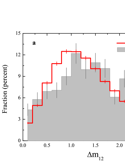
Figure 9.— Distribution of $\Delta m_{12}$(a) and $\Delta m_{14}$(b) for observational and simulation samples.

Figure 10.— Fraction of fossil groups according to both definitions $\Delta m_{12}\geq 2$ and $\Delta m_{14}\geq 2.5$, as a function of halo mass, in observational sample.

10. Discussion and Conclusion

In this study we extend the earlier observational studies of luminosity gap to low mass regime and provide observational constrains for semi-analytic models based on this observable. We extract 620 groups in SDSS DR7 utilizing mFoF algorithm and measure the luminosity gap between the two brightest galaxies in the group, $\Delta m_{12}$. This results in 109 groups with $\Delta m_{12}\geq 2$, within half a virial radius, known as optical fossils groups. In addition, Bower et al. (2006) semi-analytic model employed on Millennium simulation was used to select 16688 groups with 1993 fossil groups in the same manner as applied to the observational data. A Monte carlo simulation was also performed to generate a large sample of luminosity gap statistics purely drawn at random from Schechter luminosity function to investigate the importance of the random processes.

We show that fossil BGGs both in observations and simulations are on average brighter than those in control galaxy groups.

Given a relatively poor constrain on galaxy velocity dispersion in groups (e.g. dynamical mass estimation) we adapted the total luminosity method for the estimation of the total gravitational mass of the groups based on empirical relations. We show fossil groups halos are found to be statistically less massive than those of the control sample for a given BGG luminosity.

We confirm that the luminosity gap in systems with low richness is predominantly driven by random processes while evolutionary mechanisms are responsible for large luminosity gap in rich groups.

We find indications that the fraction of fossil groups based on $\Delta m_{14}\geq 2.5$ criterion is higher compared to the same when adopting the conventional $\Delta m_{12}\geq 2$ criterion. This is valid mostly to the low mass end.

Following a recent study by Smith et al. (2010), base on a sample of massive galaxy clusters $(\sim 10^{15}M_{\odot})$, we propose a test based on the luminosity gap in galaxy group, the butterfly diagram $M_{r}$ vs. $\Delta m_{12}$, which is found to be able to discriminate between different galaxy formation models in groups and clusters when a large sample of groups with known luminosity gap is available. Extending their study to low mass groups, we compare 620 observed groups and 16688 simulated groups in the plane of $M_{r}$ vs. $\Delta m_{12}$, Fig. 11. The absolute magnitude of the brightest and second brightest galaxy within the group are plotted as a function of $\Delta m_{12}$ for different halo masses. A linear regression is also presented for both the brightest and the second brightest galaxies as a function of $\Delta m_{12}$. In addition, Fig. 11 shows the variation of the slope and the intercept of the linear fit as a function of the halo mass for BGGs.

We find that the slope of the BGG brightness in Bower et al. (2006) simulation is steeper than the observed BGGs, particulary in high mass regime. This implies that the AGN feedback in BGG is too weak in Bower et al. (2006) semi-analytic model (Smith et al., 2010). Further improvements have been made in the semi-analytic model recently (Bower et al 2008) driven by constraints from the IGM properties of the galaxy systems, which also required a re-tuning of the galaxy formation parameters in their earlier model to be able to reconstruct the galaxy luminosity function in the local universe.

The discussion on the success of their changes in the context of the luminosity gap requires a direct comparison of the two semi-analytic models Bower et al. (2006, 2008). We find that the BGG brightness of observed groups, increases with halo mass. In contrast this trend is not clear in simulated groups. Furthermore, in high mass bin, the absolute magnitude of simulated BGG span $\sim 2.5$ mag, in contrast to the observed range of $\sim 1$ mag. Smith et al. (2010) argue that the large spread in the absolute magnitude of simulated BGGs is driven by higher efficiency of the conversion of the cold gas into stars. We note that in low mass bin, where the random processes are dominated, the spread in the luminosity of the observed and simulated BGGs are nearly the same ($\sim 0.5$ $mag$).

The correlation between the slope of the line fitted to BGG in Fig. 11 and halo mass points to an increasing contribution of the evolutionary mechanisms in forming the luminosity gap in more massive halos. Giving the considerable space density of large luminosity gap groups (e.g. Vikhlinin et al. 1999, Jones et al. 2003, van den Bosch 2007, D’Onghia et al. 2005, von Benda-Beckmann et al. 2008, Dariush et al. 2007), it seems that the butterfly diagram is a simple way of testing the accuracy of the semi-analytic models.

Figure 11.— Upper Figure shows the distribution of r-band absolute magnitude for the first (open circles) and second (filled circles) brightest group member as a function of $\triangle m_{12}$ for different halo masses. Figure at the bottom shows, the evolution of slopes and intercepts of brightest group member as a function of halo mass.

References

- Abazajian et al. (2009) Abazajian K., et al., 2009, ApJS, 182, 543
- Abell (1958) Abell, G.O., 1958, ApJS, 3,211
- Barnes (1989) Barnes, J.E., 1989, Nature, 338,123
- Beers et al. (1990) Beers, T.C., Flynn, K., Gebhardt, K., 1990, AJ, 100, 32
- Berlind et al. (2006) Berlind, A. A., et al. 2006, ApJ, 167, 1
- Blanton et al. (2003a) Blanton, M. R., et al. 2003a, AJ, 125, 2276
- Blanton et al. (2003b) Blanton, M. R., et al. 2003b, AJ, 125, 2348
- Bower et al. (1992) Bower,R., Lucey, J. R., Ellis, R. S., 1992, MNRAS, 254, 601
- Bower et al. (2006) Bower, R. G.; Benson, A. J.; Malbon, R.; Helly, J. C.;Frenk ,C. S.; Baugh, C. M.; Cole, S.; Lacei, C. G., 2006, MNRAS, 370,645
- Bower et al. (2008) Bower, R. G., McCarthy, I. G., & Benson, A. J. 2008, MNRAS, 390, 1399
- Brough et al. (2008) Brough, S., Couch, W. J., Collins, C. A., Jarrett, T., Burke, D. J., & Mann, R. G. 2008, MNRAS, 385, 103
- Colless et al. (2001) Colless, M. et al., 2001, MNRAS, 328 ,1039
- Croton et al. (2006) Croton, D.J., Springel, V., White, S.D.M., De Lucia, G.; Frenk, C. S.; Gao, L.; Jenkins, A., Kauffmann, G., Navarro, J. F., & Yoshida, N., 2006, MNRAS, 365, 11
- Dariush et al. (2007) Dariush, A., Khosroshahi, H. G., Ponman, T. J., Pearce, F.,Raychaudhury, S., & Hartley, W. 2007, MNRAS, 382, 433
- Dariush et al. (2010) Dariush, A., Raychaudhury, S., Ponman, T. J., Khosroshahi, H. G., Benson A. J., Bower R. G., & Pearce, F., 2010, MNRAS, 405, 1873
- Diaz-Gimenez et al. (2008) Diaz-Gimenez E., Muriel H., Mendes de Oliveira C., 2008, A&A, 490,965
- D’Onghia et al. (2005) D’Onghia E., Sommer-Larsen J., Romeo A. D., Burkert A., Pedersen K., Portinari L., Rasmussen J., 2005, ApJ, 630, 109
- Einasto et al. (2005) Einasto, J., Tago E., Einasto, M., Saar, E.: 2005a, In Nearby Large-Scale Structures and the Zone of Avoidance , eds. A.P. Fairall, P. Woudt, ASP Conf. Series, 329, 27
- Ellis & O’Sullivan (2006) Ellis S. C., O’Sullivan E., 2006, MNRAS, 367, 627
- Girardi et al. (1998) Girardi M., Giuricin G., Mardirossian F., Mezzetti M., Boschin W., 1998, ApJ, 505, 74
- Gladders et al. (2000) Gladders, M. D., Yee, H. K. C., 2000, AJ, 120, 2148
- Goto et al. (2005) Goto, T., et al. 2005, MNRAS, 359, 1415
- Huchra & Geller (1982) Huchra, J. P., & Geller, M. J. 1982, ApJ, 257, 423
- Jones et al. (2003) Jones, L.R, Ponman, T.J., Horton, A., Babul, A., Ebeling, H. Burke, D.J., Forbes, D.A., 2003, MNRAS, 343, 627
- Khosroshahi et al. (2006) Khosroshahi H. G., Maughan B. J., Ponman T. J., Jones L. R., 2006, MNRAS, 369, 1211
- Khosroshahi, Ponman & Jones (2006) Khosroshahi H. G., Ponman T. J., Jones L. R., 2006, MNRAS, 372, L68
- Khosroshahi et al. (2007) Khosroshahi, H.G., Ponman, T.J. & Jones, L.R., 2007, MNRAS, 377, 595
- Kodama et al. (1998) Kodama, T., & Arimoto, N. 1998, MNRAS, 300, 193
- Lin et al. (2004) Lin, Y. T., Mohr, J. J., Stanford, S. A. 2004, ApJ, 610, 745
- Merchan et al. (2005) Merchan M., Zandivarez A., 2005, ApJ, 630, 759
- Miller et al. (2005) Miller, C. J., et al. 2005, AJ, 130, 968
- Milosavljevic et al. (2006) Milosavljevic, M., Miller C. J., Furlanetto R., Cooray A., 2006, ApJ, 637, 9
- Oyaizu et al. (2008) Oyaizu, H., et al. 2008, ApJ, 2008, 674, 768
- Paredes et al. (1995) Paredes S., Jones B. J. T., Martinez V. J., 1995, MNRAS, 276, 1116
- Peebles et al. (2002) Peebles, P. J. E. 2002, in ASP Conf. Ser. 283, A New Era in Cosmology, ed. N. Metcalfe & T. Shanks (San Francisco: ASP), 351
- Petrosian (1976) Petrosian, V. 1976, ApJ, 210, 53
- Popesso et al. (2005) Popesso, P., Biviano, A., Bhringer, H., Romaniello, M., Voges, W. 2005, A&A, 433, 431
- Ponman et al. (1994) Ponman, T.J., Allan, D.J., Jones, L.R., Merrifield, M. MacHardy, I.M., 1994 Nature, 369, 462
- Santos et al. (2007) Santos,W.A., Mendes de Oliveira, C., & Sodré, L., 2007, AJ, 134, 1551
- Schechter (1976) Schechter P., 1976, ApJ, 203, 297
- Schlegel et al. (1998) Schlegel, D. J., Finkbeiner, D. P., & Davis, M. 1998, ApJ, 500, 525
- Smith et al. (2010) Smith, G.P., Khosroshahi, H.G., Dariush, A., Sanderson, A.J.R., Ponman, T.J., Stott, J.P., Haines, C.P., Egami, E., Stark, D.P., 2010, ,MNRAS,in press,arXive:1007.2196S
- Spergel et al. (2003) Spergel, D. N. et al., 2003, ApJS, 148, 175
- Springel et al. (2001) Springel, V., White, S.D.M., Tormen, G., & Kauffmann, G., 2001, MNRAS, 328, 726
- Springel et al. (2005) Springel, V. et al., 2005, Nature, 435, 629
- Strauss et al. (2002) Strauss, M. A. et al. 2002, AJ, 124, 1810
- Struble et al. (1987) Struble M.F., Rood H.J. 1987, ApJS, 63, 555
- Tago et al. (2008) Tago, E. et al. 2008, A&A, 479, 927-937
- van den Bosch (2007) van den Bosch F. C. et al. 2007, MNRAS, 376, 841
- Vikhlinin et al. (1999) Vikhlinin, A.,McNamara, B.R., Hornstrup, A., Quintana, H., Forman, W., Jones, C. Way, M., 1999, ApJ, 520, 1
- Voges et al. (1999) Voges, W., et al. 1999, A&A, 349, 389