A new approach to the vacuum of inflationary models

Abstract

A new approach is given for the implementation of boundary conditions used in solving the Mukhanov-Sasaki equation in the context of inflation. The familiar quantization procedure is reviewed, along with a discussion of where one might expect deviations from the standard approach to arise. The proposed method introduces a (model dependent) fitting function for the $z^{\prime\prime}/z$ and $a^{\prime\prime}/a$ terms in the Mukhanov-Sasaki equation for scalar and tensor modes, as well as imposes the boundary conditions at a finite conformal time. As an example, we employ a fitting function, and compute the spectral index, along with its running, for a specific inflationary model which possesses background equations that are analytically solvable. The observational upper bound on the tensor to scalar ratio is used to constrain the parameters of the boundary conditions in the tensor sector as well. An overview on the generalization of this method is also discussed.

I Introduction

As is well known, the inflationary paradigm provides solutions to many cosmological problems such as the flatness problem, the horizon or causality problem, and also dilutes unwanted (and unobserved) relics Guth ; Linde ; Steinhardt . It also provides a natural mechanism of producing primordial perturbations that seed the inhomogeneities of the universe Mukhanov pert ; sasaki pert . The basic idea is that the quantum fluctuations of a classically homogeneous scalar field, the inflaton, source quantum fluctuations of the spacetime metric (the inflaton will create density perturbations which will source the scalar fluctuations of the metric). During the process of inflation, this quantum fluctuation is amplified to become a classical fluctuation, and, at the end of inflation, the fluctuation in the metric induces the density fluctuations of matter that were produced during reheating . This primordial perturbation generated during inflation then is what gives rise to the formation of structure in the universe.

In this story, the crucial quantities to be determined are the amplitude of the primordial density and tensor perturbations, as the growth of structure is dependent on their size. The subsequent evolution of the primordial perturbations can be inferred from careful observations of the history of the growth of structure. From this we expect that the density perturbation produced by inflation to be $\mathcal{O}(10^{-5})$.

Therefore, it is important to be able to accurately compute these perturbations in order to either preserve or rule out a given inflationary model. For the usual models of inflation, Ricci scalar plus a single canonically normalized scalar field, there are two components that will determine this amplitude. As will be described in more detail below, the first is the form of a function, $z^{\prime\prime}/z$, which arises in the Mukhanov-Sasaki equation. This equation is satisfied by a mode function, $v_{k}$, which arises by a redefinition of the co-moving curvature perturbation in momentum space, $\mathcal{R}_{k}$, upon having written the original action in terms of $\mathcal{R}_{k}$. Since this equation is crucial to finding the curvature perturbation (the same equation is also obeyed by the tensor modes), it is essential that one accurately specifies its form.

The second component is the input from vacuum selection, which is equivalent to a boundary condition for the Mukhanov-Sasaki equation. For example, one avenue of study has been to alter the initial state to lie away from the standard Bunch-Davies vacuumBunchDavies ; Danielsson trans Planck ; New Physics CMB ; Easther:2005a ; Chen:2006a ; Holman:2007a ; Meerburg:2009a ; Padmanabhan ; Ashoorioon:2012 . Such alternative boundary conditions are typically chosen by conditions set at a given cut-off scale in either momentum or time. These choices will then manifest themselves in physical observables (for example as new features in the power spectrum, or enhanced non-Gaussianity) which can allow one to gain knowledge of the initial state from observation. It should be mentioned that there exist arguments Susskind that the Bunch-Davies vacuum might be the most probable vacuum to produce the correct power spectrum from the perspective of technical naturalness, although this does not eliminate the possibility of deviations from the Bunch-Davies vacuum.

It is customary to characterize inflation as a period of time where the scale factor grew almost exponentially, a period called de Sitter or quasi-de Sitter inflation (exact exponential growth of the scale factor, $a\propto e^{Ht}$, with $H$ constant, is technically de Sitter inflation, and nearly exponential growth is termed quasi-de Sitter). If the universe inflates as a power law manner $a\varpropto\tau^{p}$ where $\tau$ is the conformal time and $p$ is a constant, than the solution of the Mukahanov-Sasaki equation is known. Notice that de Sitter inflation correspond to $p=-1.$ The solution for general $p$ is given by a linear combination of Bessel functions. The calculation for the perturbation amplitude has been well established for such a case.Lyth and Stewart However, for most models of inflation, power law expansion happens only in a short period of time either at the beginning or the end of the inflation. Thus this commonly used approximation may not apply to all inflationary models. If one insists on using the equations derived from the power law limit, one runs the risk of possibly ruling out phenomenologically viable models, or of preserving models that are ruled out by observational data.

In the present work we would like to address the possibility that the function $z^{\prime\prime}/z$ inside the Mukhanov equation deviates from the de Sitter limit, and how that may affect one’s choice of boundary conditions. It may be that before some point $\tau_{p}$ that using the de Sitter limit is not consistent, and therefore placing boundary conditions at $\tau_{p}$ is more natural. We have thus expanded the standard method of computing the amplitude of the primordial perturbation for such a case. Our method applies to those inflationary models that do not behave with power law (at least partially) expansion with some specific constraints in the background evolution.

The paper is organized as follows. In Sec.II we review the standard calculation of primordial density and tensor perturbations where the de Sitter limit is taken. We also explain the physical reasons behind the commonly chosen Bunch-Davies vacuum. In Sec.III we introduce a new method of vacuum selection by applying this method to a specific inflation model. The principles of generalizing this method to other models is also given. In Sec.IV we give our conclusions.

II The standard method

We will now outline the key ingredients for the calculation of the primordial perturbations by quantizing the comoving curvature perturbation as well as the tensor perturbation Lyth and Stewart (for a recent textbook treatment and lecture notes see Weinberg:2008 ). The theories we consider here contain an Einstein-Hilbert action and a canonically normalized scalar field, minimally coupled to gravity with an arbitrary self-interacting potential

$$S=\int d^{4}x\sqrt{-g}\left\{\frac{1}{2\kappa^{2}}R-\frac{1}{2}g^{\mu\nu}\partial_{\mu}\sigma\partial_{\nu}\sigma-V\left(\sigma\right)\right\}$$ (1)

where $\kappa^{2}=8\pi G=1/M_{Pl}^{2}$ and our metric signature is $-+++$.

II.1 Scalar Perturbations

We begin with the perturbed Friedmann-Robertson-Walker(FRW) metric including the most general perturbations

$$ds^{2}=a^{2}(\tau)\{-(1+2A)d\tau^{2}-2\partial_{i}Bdx^{i}d\tau+\left[\left(1+2\mathcal{R}\right)\delta_{ij}+\partial_{i}\partial_{j}H_{T}\right]dx^{i}dx^{j}\}$$ (2)

Where $A\left(\tau,\mathbf{x}\right),B\left(\tau,\mathbf{x}\right),\mathcal{R}\left(\tau,\mathbf{x}\right)$ and $H_{T}$ $\left(\tau,\mathbf{x}\right)$ are small perturbations around homogeneous FRW metric. We will be concerned with calculating the scalar $\mathcal{R}$, which is the gauge invariant comoving curvature perturbation.

Variation of the action Eq.(1) gives the Einstein equations and the scalar field equation of motion, which at the background level are

$$\frac{\left(a^{\prime}\right)^{2}}{a^{4}}=\frac{\kappa^{2}}{3}\left[\frac{1}{2a^{2}}\left(\sigma^{\prime}\right)^{2}+V\left(\sigma\right)\right]$$ (3)

$$\frac{a^{\prime\prime}}{a^{3}}-\frac{\left(a^{\prime}\right)^{2}}{a^{4}}=-\frac{\kappa^{2}}{3}\left[\frac{1}{a^{2}}\left(\sigma^{\prime}\right)^{2}-V\left(\sigma\right)\right]$$ (4)

$$\frac{\sigma^{\prime\prime}}{a^{2}}+2\frac{a^{\prime}}{a^{3}}\sigma^{\prime}+V^{\prime}\left(\sigma\right)=0$$ (5)

where a prime denotes a derivative with respect to the conformal time, $\tau$, while a dot will indicate a derivative with respect to the coordinate time, $t$.

Putting the solutions for the background evolution back into the Einstein-Hilbert action, and expanding the action to second order in the perturbations gives (setting $\kappa^{2}=1$)

$$S_{(2)}=\frac{1}{2}\int d^{4}xa^{3}\frac{\dot{\sigma}^{2}}{H^{2}}\left[\mathcal{\dot{R}}^{2}-a^{-2}\left(\partial_{i}\mathcal{R}\right)^{2}\right].$$ (6)

The above expression can be obtained using the gauge symmetry in the action to choose $\delta\sigma=0.$ One may define the Mukhanov variable

$$v\equiv z\mathcal{R},\text{ \ \ where \ \ \ }z^{2}\equiv a^{2}\frac{\dot{\sigma}^{2}}{H^{2}}=-2a^{2}\frac{\dot{H}}{H^{2}}\equiv 2a^{2}\epsilon.$$ (7)

We have introduced the slow-roll parameter $\epsilon$. The second order action can be rewritten as

$$S_{\left(2\right)}=\frac{1}{2}\int d\tau d^{3}x\left[\left(v^{\prime}\right)^{2}-\left(\partial_{i}v\right)^{2}+\frac{z^{\prime\prime}}{z}v^{2}\right].$$ (8)

To quantize this action first define the canonical conjugate momentum of $v$, and then impose the usual commutation relation

$$\Pi_{v}=\frac{\partial L}{\partial v^{\prime}}=v^{\prime};\ \ \left[v(\tau,\mathbf{x}),\Pi_{v}(\tau,\mathbf{x}^{\prime})\right]=i\hbar\delta^{\left(3\right)}(\mathbf{x}-\mathbf{x}^{\prime}).$$ (9)

Henceforth we shall set $\hbar=1$.

Now one performs a plane-wave expansion of the now quantum operator $\hat{v}(\tau,\vec{x})$ in Fourier space

$$\hat{v}(\tau,\vec{x})=\int\frac{d^{3}\mathbf{{k}}}{(2\pi)^{3}}[v_{k}(\tau)\hat{a}_{\mathbf{k}}e^{i\mathbf{k}\cdot\mathbf{x}}+v_{k}^{\ast}(\tau)\hat{a}_{\mathbf{k}}^{\dagger}e^{-i\mathbf{k}\cdot\mathbf{x}}]$$ (10)

Requiring the canonical commutation relation between $\hat{a}_{\mathbf{k}}(\tau)$ and $\hat{a}_{\mathbf{k}}^{\dagger}(\tau)$, $[\hat{a}_{\mathbf{k}}(\tau),\hat{a}_{\mathbf{k}^{\prime}}^{\dagger}(\tau)]=(2\pi)^{3}\delta^{(3)}(\mathbf{k}-\mathbf{k}^{\prime})$, we will obtain the Wronskian condition for the mode function $v_{k}(\tau)$

$$\left(v_{k}^{\ast}v_{k}^{\prime}-v_{k}^{\prime\ast}v_{k}\right)=-i\text{ }$$ (11)

The mode function in momentum space satisfies the Mukhanov-Sasaki equation

$$v_{k}^{\prime\prime}\left(\tau\right)+\left(k^{2}-\frac{z^{\prime\prime}}{z}\right)v_{k}\left(\tau\right)=0\text{ }$$ (12)

Upon introducing the second slow-roll parameter

$$\eta=-\frac{\overset{\cdot\cdot}{\sigma}}{H\dot{\sigma}}$$ (13)

one can express $\frac{z^{\prime\prime}}{z}$ in terms of the first and second slow-roll parameters

$$\frac{z^{\prime\prime}}{z}=2a^{2}H^{2}\left(1-\frac{3}{2}\eta+\epsilon+\frac{1}{2}\eta^{2}-\frac{1}{2}\epsilon\eta+\frac{1}{2H}\dot{\epsilon}-\frac{1}{2H}\dot{\eta}\right)$$ (14)

In general, Eq.$\left(\ref{Muk}\right)$ with $z^{\prime\prime}/z$ given in Eq.$\left(\ref{z''/z}\right)$ is difficult to solve analytically. For a special subset of general theories where $\epsilon$ and $\eta$ are approximately constants, the equation is analytically solvable. In this special case $z^{\prime\prime}/z$ can be written as

$$\frac{z^{\prime\prime}}{z}=\frac{\nu^{2}-\frac{1}{4}}{\tau^{2}}\text{ \ \ where \ }\nu=\frac{1-\eta+\epsilon}{1-\epsilon}+\frac{1}{2}$$ (15)

and the analytic solution for $v_{k}\left(\tau\right)$ is given in terms of Bessel functions

$$v_{k}\left(\tau\right)=\alpha\sqrt{\tau}J_{\nu}\left(k\tau\right)+\beta\sqrt{\tau}Y_{\nu}\left(k\tau\right)$$ (16)

Where $\alpha$ and $\beta$ are two complex parameters. A well known example for this special case is that of power law inflation, $a=c\tau^{p},$ where $\epsilon=\eta=\frac{p+1}{p}$. One then obtains $z=\sqrt{\frac{2c^{2}(p+1)}{p}}\tau^{p}$, which gives $z^{\prime\prime 2}$ or $\nu=-p+1/2,$ and the comoving horizon ${(aH)}^{-1}=\tau/p$. Pure de Sitter expansion is the specific case of $p=-1$. For genuine de Sitter inflation, $z$ vanishes, which leads to an exactly scale-invariant power spectrum that is now observationally disfavored Komatsu:2010 . This implies that inflation must deviate from the pure de Sitter case.

The solutions to Eq.$(\ref{Muk})$ can be written either as linear combinations of Bessel functions, $J_{n}(x)$ and $Y_{n}(x)$, or Hankel functions, $H_{n}^{(1)}(x)$ and $H_{n}^{(2)}(x)$

$$v_{k}\left(\tau\right) =\alpha\sqrt{\tau}J_{-p+\frac{1}{2}}\left(k\tau\right)+\beta\sqrt{\tau}Y_{-p+\frac{1}{2}}\left(k\tau\right)$$ (17)

$$=\widetilde{\alpha}\sqrt{\tau}H_{-p+\frac{1}{2}}^{\left(1\right)}\left(k\tau\right)+\widetilde{\beta}\sqrt{\tau}H_{-p+\frac{1}{2}}^{\left(2\right)}\left(k\tau\right)$$ (18)

The Wronskian condition Eq.$(\ref{normalization})$ requires

$$\alpha^{\ast}\beta-\alpha\beta^{\ast}=-\frac{i\pi}{2}\text{ or }\left|\widetilde{\alpha}\right|^{2}-\left|\widetilde{\beta}\right|^{2}=1\text{ }$$ (19)

When the solution is expressed in terms of Hankel functions, there is a natural place where the boundary condition may be imposed, that is when $\left|k\tau\right|\gg 1$, or equivalently when the comoving wavelength is deep inside the comoving Hubble radius. The asymptotic forms of the Hankel functions become positive and negative frequency modes

$$\lim_{\left|k\tau\right|\gg 1}\sqrt{\tau}H_{-p+\frac{1}{2}}^{(2)}(k\tau)=e^{-ik\tau}\,\,;\,\,\lim_{\left|k\tau\right|\gg 1}\sqrt{\tau}H_{-p+\frac{1}{2}}^{(1)}(k\tau)=e^{ik\tau}.$$ (20)

The fact that in the far past the solution approaches those of Minkowski space can be seen in the behavior of $z^{\prime\prime}/z$ displayed in Fig.$(\ref{zppzfit})$

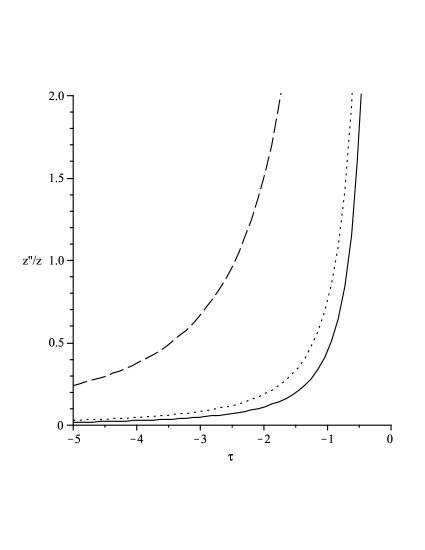
Figure 1: A plot of $p(p-1)/\tau^{2}$ for the cases: $p=-2$ given by the dashed line, $p=-1/2$ given by the dotted line, and $p=-1/3$ given by the solid line.

The vanishing behavior of $z^{\prime\prime}/z$ in this asymptotic region ensures that solutions to Eq.$(\ref{Muk})$ reduce to the Minkowski type in the far past. Thus, for these classes of inflationary models there is a natural boundary condition that the solution should approach the positive frequency ougoing mode with no incoming modes

$$\lim_{\tau\rightarrow-\infty}v_{k}(\tau)=\frac{e^{-ik\tau}}{\sqrt{2k}}$$ (21)

This form is seen to match that of $H_{p-\frac{1}{2}}^{(1)}(k\tau)$ in Eq.(20). The boundary condition Eq.(21) is known as the Bunch-Davies vacuum BunchDavies . This has the effect of setting $\tilde{\alpha}=1$ and $\tilde{\beta}=0$ in Eq.(17). This appears as a natural choice, as one may think intuitively that at the beginning of time, all the particles (or positive frequency modes) should move forward in time, thus eliminating the possibility of having a contribution from the $H_{p-\frac{1}{2}}^{(2)}(k\tau)$ term.

We would like to stress that although $\tau\rightarrow-\infty$ is a legitimate limit formally, but physically there will exist a time where the physical wavelength will be comparable to the Planck length where quantum gravity effects should take place. This means in that region, the background evolution can no longer be treated classically. Due to the lack of a full quantum gravity theory, the boundary condition may be imposed at some later time where the physical wavelength is greater than the Planck length. The effect of setting the boundary condition at a finite time may be that the state does not reside in the ground state, but rather in some squeezed or distorted state Danielsson trans Planck ; New Physics CMB ; Grishchuk:1993 .

For general energy contents of the universe, the form of the scale factor will no longer be a simple power-law (although during times where a single component is the dominant contributor to the stress-energy such as during matter or radiation domination, the power-law form is a good approximation). As an approximation, a standard analytic approach is to assume the expansion is approximately de Sitter, $p\approx-1$, and therefore $\epsilon\approx 0$ . Together with the smallness condition of the second slow-roll parameter $\eta=-\frac{\overset{\cdot\cdot}{\sigma}}{H\dot{\sigma}}\ll 1$ using Eq.$\left(\ref{standard fit}\right)$ one finds

$$\frac{z^{\prime\prime}}{z}\approx\frac{a^{\prime\prime}}{a}\approx\frac{2}{\tau^{2}}$$ (22)

Under this assumption, the solution of the Mukhanov-Sasaki equation is

$$v_{k}\left(\tau\right)=\tilde{\alpha}\sqrt{k\tau}H_{3/2}^{(1)}(k\tau)+\tilde{\beta}\sqrt{k\tau}H_{3/2}^{(2)}(k\tau)$$ (23)

where $\tilde{\alpha}$ and $\tilde{\beta}$ are two complex parameters with four degrees of freedom, one of which is fixed by Eq.(19), two more by Eq.(21), leaving one irrelevant phase undetermined. With these conditions, the solution for the mode function is

$$v_{k}\left(\tau\right)=\frac{e^{-ik\tau}}{\sqrt{2k}}\left(1-\frac{i}{\kappa\tau}\right)$$ (24)

This leads to the well known relations for the scalar power-spectrum, $P_{\mathcal{R}}$, the spectral index $n_{s}$, and the running of the spectral index $\alpha_{s}$

$$P_{\mathcal{R}}\equiv\left.\frac{\left|v_{k}(\tau)\right|^{2}}{z^{2}}\right|_{k=aH}=\left.\frac{H^{2}}{4k^{3}\epsilon}\right|_{k=aH}$$ (25)

$$n_{s}-1\equiv\left.\frac{d\ln(k^{3}P_{\mathcal{R}})}{d\ln k}\right|_{k=aH}=\left.\frac{k}{k^{3}P_{\mathcal{R}}}\frac{d(H^{2}/\epsilon)}{d\tau}\frac{d\tau}{dk}\right|_{\tau=\tau_{\ast}}$$ (26)

$$\alpha_{s}\equiv\left.\frac{dn_{s}}{d\ln k}\right|_{k=aH}$$ (27)

Note that each relation is to be evaluated at horizon crossing, $k=aH$ (or equivalently $\tau=\tau_{\ast}$), due to the fact that the perturbation is frozen when the comoving wavelength becomes stretched outside the comoving Hubble radius.

The accuracy of this program strongly depends on the quality of how well the approximation of the curve $z^{\prime\prime}/z$ compares with the true function $z^{\prime\prime}/z$ . Applying these equations to models where $z^{\prime\prime}/z$ is not well fit by the power law and slow-roll approximations may result in serious deviations from the observable predictions. This is precisely the problem we will address in Section III. Before doing so we will first give an overview of quantization in the tensor sector.

II.2 Tensor Perturbations

The calculation for tensor perturbations mirrors that of the scalar perturbation. The starting point is once again the perturbed FRW metric with a transverse, traceless tensor perturbation, $h_{ij}$ (we have omitted the scalar and vector perturbations seen previously which has no effect on the tensor mode evolution due to decoupling of the scalar, vector, and tensor sectors)

$$ds^{2}=a^{2}\left(-d\tau^{2}+\left(\delta_{ij}+h_{ij}(\mathbf{x},\tau)\right)dx^{i}dx^{j}\right)$$ (28)

Next, one expands the Einstein-Hilbert action to second order in the perturbation

$$S_{\left(2\right)}=\frac{M_{pl}^{2}}{8}\int d\tau dx^{3}a^{2}\left[(h_{ij}^{\prime}(\mathbf{x},\tau))^{2}-(\partial_{l}h_{ij}(\mathbf{x},\tau))^{2}\right]$$ (29)

As in the scalar case, one expands $h_{ij}$ in Fourier space in terms of plane waves with modes $h_{\mathbf{k}}^{s}$

$$h_{ij}(\mathbf{x},\tau)=\int\frac{d^{3}k}{(2\pi)^{3}}\sum_{s=\times,\,+}\epsilon_{ij}^{s}h_{\mathbf{k}}^{s}(\tau)e^{i\mathbf{k}\cdot\mathbf{x}}$$

where $\epsilon_{ij}^{s}$ are the spin-two polarization tensors. One can then make the definition

$$\mu_{k}^{s}\left(\tau\right)=\frac{1}{2}ah_{k}^{s}\left(\tau\right)$$ (30)

which leads to the action (here we have set $M_{Pl}=1$)

$$S_{\left(2\right)}=\sum_{s}\frac{1}{2}\int d\tau d^{3}k\left[\left(\mu_{k}^{s\prime}\right)^{2}-\left(k^{2}-\frac{a^{\prime\prime}}{a}\right)\left(\mu_{k}^{s}\right)^{2}\right]$$ (31)

This action gives similar equations of motion as Eq.$\left(\ref{Muk}\right)$

$$\mu_{k}^{s\prime\prime}\left(\tau\right)+\left(k^{2}-\frac{a^{\prime\prime}}{a}\right)\mu_{k}^{s}\left(\tau\right)=0\text{ }$$ (32)

For a scale factor of the power-law form, the calculation follows exactly as in the scalar case while the fit function in terms of slow-roll parameter is now

$$\frac{a^{\prime\prime}}{a}=\frac{\mu^{2}-\frac{1}{4}}{\tau^{2}}\text{ \ \ where }\mu=\frac{1}{1-\epsilon}+\frac{1}{2}.$$ (33)

In the case of quasi de Sitter inflation, $\epsilon\approx 0$, the power spectrum for a single polarization of the tensor modes toward the end of inflation is

$$P_{t}=\left.4\frac{\left|\mu_{k}\right|^{2}}{a^{2}}\right|_{k=aH}=\left.\frac{2H^{2}}{k^{3}}\right|_{k=aH}$$ (34)

which differs from the form of the scalar result in that the slow-roll parameter $\epsilon$ is absent in the denominator. The full power spectrum is then twice this (due to two polarization states) $P_{h}=2P_{t}=4H^{2}/k^{3}$, which leads to a small tensor to scalar ratio $r=P_{h}/P_{\mathcal{R}}=16\epsilon$ when the slow-roll parameter is small.

These results for the power spectra are obtained under the assumption that the expansion is de Sitter or very nearly de Sitter in the sense that Eq.(22) is true. To obtain a more accurate predication one must solve the Mukhanov equation on a model-by-model basis using the exact $z^{\prime\prime}/z$ (or $a^{\prime\prime}/a$) numerically, along with choosing a proper boundary condition accordingly. In the next section we will institute such a procedure in order to quantize models where Eq.$(\ref{desitter})$ is not a good approximation.

III Vacuum Selection

The mode equation one needs to solve is

$${v}_{k}^{\prime\prime 2}-f(\tau))v_{k}=0$$ (35)

One can obtain the analytic expression for $f(\tau)$ from solving the background equations. For the scalar case $f(\tau)$ is given by $z^{\prime\prime}/z$, while for the tensor case it is $a^{\prime\prime}/a$. In the de Sitter limit, its value is shown in Eq.(22). In general, the background evolution is not tractable analytically, and for the few cases where the background solution is analytically solvable analytic background ; analytic Easther ; analytic Barrow ; analytic Barrow2 ; analytic Ellis and Madsen ; analytic Easther2 ; analytic Lidsey ; analytic Mimoso , the $\tau$ dependence in $f(\tau)$ may be so complicated that finding an analytic solution for Eq.(35) becomes impossible. It is worth mentioning that the equation is equivalent to a time independent Schrodinger equation in one dimension when $\tau$ is regarded as space coordinate and $f\left(\tau\right)$ is the potential for the wave function $v_{k}\left(\tau\right).$ This analogy will become apparent when we introduce our method of solving Eq.$\left(\ref{master}\right)$, which is nothing but the usual WKB approximation in quantum mechanics.

Under the condition that the background evolution of the metric is known for a particular inflationary model, one can determine whether the approximation Eq.(22) will be applicable for the model under consideration. If so, then the system may be solved using the standard approach outlined in the preceding section. However, this is not the case for a great number of inflationary models. One can understand that this is so because the mechanism used in stopping inflation may falsify the standard approximation. Additionally, the initial conformal time can not always be pushed back to negative infinity where one would impose the Bunch-Davies boundary condition as is the case when the expansion is truly power-law.

The essential idea of our method is that, since the information one needs in order to calculate observables to compare with experiment is the value of the mode function at horizon crossing (which is much later than the asymptotic time $\tau\rightarrow-\infty$), it may therefore be advantageous to place the physical boundary condition closer to the time where we require accurate information. Imposing the boundary condition at negative infinity may lead to a situation where the approximate form for $f(\tau)$ in Eq.(22) has deviated greatly from the actual solution due to the lengthy intervening period of evolution. Although we are placing the boundary condition nearer the era of observable inflation, we will continue to mimic the idea of BD vacuum selection in that we look at the time $\tau=p$ where the wavelength of the mode is deep inside the horizon, and the effect of cosmic expansion is relatively small. The situation can then be approximated as physics in Minkowski space.

In this section we will first demonstrate the method with an explicit example before going on to comment on considerations on applying the method in general.

III.1 A Specific Example

The model we use as an example has background evolution that is analytically solvable analytic background . This particular model provides an interesting picture where the Big Bang is connected to inflation with a specific time delay. The behavior of $z^{\prime\prime}/z$ is very different from the slow roll plus de Sitter limit, while the term $a^{\prime\prime}/a$ is asymptotically equal to the de Sitter limit. We will apply our method to obtain the scalar power spectrum and constrain the tensor power spectrum from observation.

Our point here is to show that there exist examples such that $z^{\prime\prime}/z$ can not be approximated by the standard fit function, thus there is a need of introducing new method of solving Mukhanov-Sasaki equation. We would like to point out this model does not provide a mechanism of stopping inflation, therefore, even though our method predicts the correct power spectrum in a certain parameter space, the phenomenologically viable parameter space is expected to change when the stopping mechanism is introduced. Therefore the model in question may be viewed as a demonstration tool (due to the attractive property that it is analytically solvable at the background level) rather than a fully complete model.

We begin with an action of the form Eq.$\left(\ref{action}\right)$ with the scalar potential

$$V\left(\sigma\right)=\left(\frac{6}{\kappa^{2}}\right)^{2}\left(c\sinh^{4}\left(\sqrt{\frac{\kappa^{2}}{6}}\sigma\right)+b\cosh^{4}\left(\sqrt{\frac{\kappa^{2}}{6}}\sigma\right)\right)$$ (36)

The potential contains the dimensionless free parameters $b$ and $c$, and $\kappa^{-1}$ is the reduced Planck mass as before. The background solution for all possible combinations of $c$ and $b$ has been classified in analytic background . We will use the case $c=64b>0$ as an example to illustrate our method.

The behavior of the scale factor of this model is to initiate expansion at $\tau=\tau_{BB}\approx 0.92$ where the scale factor is exactly zero. Beginning at a later time, $\tau_{I}$ $\approx 2.87$, there is an inflationary period, and finally, when $\tau$ approaches $\tau_{\infty}\approx 7.4$, the scale factor diverges. At this point the physical time, $t=\int a\left(\tau\right)d\tau$, will also diverge. Of course the finite value $\widetilde{\tau}_{BB}\approx 0.92$ is not physically significant since $\tau$ can be translated by an arbitrary amount. The solutions for the background evolution of the scale factor $a\left(\tau\right)$ and inflaton $\sigma(\tau)$ are as follows

$$a\left(\tau\right)=\sqrt{\frac{1}{12}}\kappa\left(\frac{E}{b}\right)^{\frac{1}{4}}\left\{2\left[\frac{1-cn\left(\frac{1}{2}\widetilde{\tau}\right)}{1+cn\left(\frac{1}{2}\widetilde{\tau}\right)}\right]-\frac{1}{4}\left[cn\left(\widetilde{\tau}\right)\right]^{2}\right\}^{\frac{1}{2}}$$ (37)

and

$$\sigma\left(\tau\right)=\frac{1}{\kappa}\sqrt{\frac{3}{2}}\ln\left(\frac{1+\frac{1}{2\sqrt{2}}cn\left(\widetilde{\tau}\right)\left[\frac{1+cn\left(\frac{1}{2}\widetilde{\tau}\right)}{1-cn\left(\frac{1}{2}\widetilde{\tau}\right)}\right]^{\frac{1}{2}}}{1-\frac{1}{2\sqrt{2}}cn\left(\widetilde{\tau}\right)\left[\frac{1+cn\left(\frac{1}{2}\widetilde{\tau}\right)}{1-cn\left(\frac{1}{2}\widetilde{\tau}\right)}\right]^{\frac{1}{2}}}\right)$$ (38)

where $\widetilde{\tau}\equiv 2\left|cE\right|^{\frac{1}{4}}\tau$. $E$ is a free parameter of this model which determines the scale of $a$, therefore $E$ can be chosen so that $a$ is normalized in the conventional way, $a\left(today\right)=1$. In the present application we will choose $E$ so that

$$2\left|cE\right|^{\frac{1}{4}}=1\text{ \ or \ }\widetilde{\tau}\equiv\tau.$$ (39)

The term $cn\left(\frac{1}{2}\widetilde{\tau}\right)\equiv cn\left(\frac{1}{2}\widetilde{\tau}|\frac{1}{2}\right)$ is the Jacobi elliptic functionabramcwtz . Following the standard method, one needs to determine whether $\epsilon$ and $\eta$ are approximately constants. If so, following Eqs.$\left(\ref{standard fit}\right)$ and $\left(\ref{tensor fit}\right)$, one can determine the fit function of $z^{\prime\prime}/z$ and $a^{\prime\prime}/a$. Since the analytic solution of this model is known, we can plot the exact curves for $\epsilon$ and $\eta$ as in Fig.2 and Fig.3).

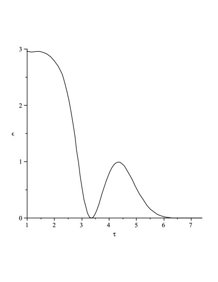
Figure 2: The slow-roll parameter $\epsilon$ as a function of conformal time.

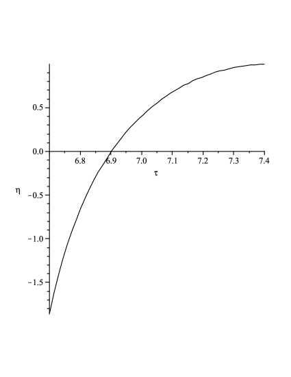
Figure 3: The slow-roll parameter $\eta$ as a function of conformal time.

One can easily see that the asymptotic values of $\epsilon$ and $\eta$ approach the constant values $0$ and $1$ respectively. These values will result in the breakdown of Eq.(15) for $z^{\prime\prime}/z$ and $2/(\tau-\tau_{\infty})^{2}$ for $a^{\prime\prime}/a$. From the above expression we can also compute $z^{\prime\prime}/z$ and $a^{\prime\prime}/a$. The result is shown in the following plots along with the fitting function

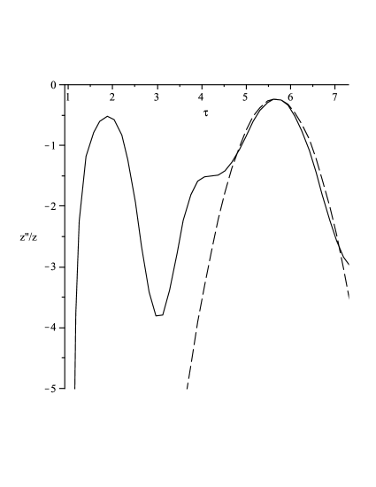
Figure 4: A plot of the function $z^{\prime\prime}/z$ as a function of conformal time. The solid line is the actual value of the function $z^{\prime\prime}/z$, and the dashed line gives the fit function.

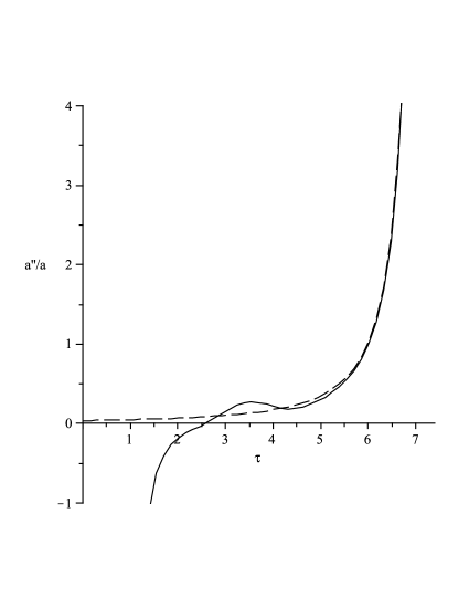
Figure 5: A plot of the function $a^{\prime\prime}/a$ as a function of conformal time. The solid line is the actual value of the function $a^{\prime\prime}/a$, and the dashed line gives the fit function.

The fit function plotted in Fig.$(5)$ is the predicted fit function for $a^{\prime\prime}/a$ which is
$2/(\tau-7.4)^{2}$, while the fit function for Fig.$\left(4\right)$ is a quadratic function

$$f_{fit}(\tau)=m(\tau-p)^{2}+h$$ (40)

with parameters

$$m=-1.2,p=5.66,h=-0.23$$ (41)

In the case of the scalar perturbation, since the formula for the standard fit function breaks down, we now introduce a new quadratic fit function according to the following rules. The parameter $p$ is designed to match the point where $f(\tau)$ has slope zero while $h$ is designed to match the value of $f\left(\tau\right)$ at $\tau=p$. The value of $m$ is the only parameter in the fit function, but it has to be adjusted such that the curve of $f_{fit}(\tau)$ approaches the actual $f\left(\tau\right)$ in the region of physical interest, namely the region where the mode exits the horizon. That is to say we want a better fit for $\tau>p$. The region $\tau<p$ corresponds to the time before the beginning of observable inflation, or before about 60 e-folds before the end of inflation. The perturbation generated during the preceding periods have yet to re-enter our horizon, thus they have produced no observable effect. (Since the universe is currently accelerating again, it is not clear to what extent regions corresponding to time intervals before the last 60 e-folds will contribute to observable effects in the future.)

Once the fit function is chosen, one can then proceed to solve the Mukhanov-Sasaki equation with the new fit function. In the current example, the two independent solutions to Eq.$\left(\ref{master}\right)$ with $f\left(\tau\right)=f_{fit}\left(\tau\right)$ are the hypergeometric functions $S_{k1}$ and $S_{k2}$. The general mode function is thus

$$v_{k}\left(\tau\right)=\alpha S_{k1}\left(\tau\right)+\beta S_{k2}\left(\tau\right)$$

where $\alpha$ and $\beta$ are two complex parameters that can be parametrized by four real parameters

$$\alpha=r_{1}e^{i\theta_{1}},\beta=r_{2}e^{i\theta_{2}}$$ (42)

written in the real parameters

$$v_{k}\left(\tau\right)=e^{i\theta_{1}}\left(r_{1}S_{1}+r_{2}e^{i\left(\theta_{2}-\theta_{1}\right)}S_{2}\right)$$ (43)

$r_{1},r_{2},\theta_{1},\theta_{2}$ are to be determined by the boundary conditions. It can be easily seen that when the quantity of interest is the expectation value of $v_{k}\left(\tau\right)$ the parameter $\theta_{1}$ is an irrelevant phase.

The exact solutions $S_{k1}$ and $S_{k2}$ are

$$S_{k1}\left(\tau\right) =e^{\left(-\frac{\tau}{2}+p\right)\sqrt{m}\tau}hypergeom\left(\frac{-1}{4}\frac{-\sqrt{m}+k^{2}-h}{\sqrt{m}},\frac{1}{2},\sqrt{m}\left(\tau-p\right)^{2}\right)$$ (44)

$$S_{k2}\left(\tau\right) =\left(\tau-p\right)e^{\left(-\frac{\tau}{2}+p\right)\sqrt{m}\tau}hypergeom\left(\frac{-1}{4}\frac{-3\sqrt{m}+k^{2}-h}{\sqrt{m}},\frac{3}{2},\sqrt{m}\left(\tau-p\right)^{2}\right)$$ (45)

where the hypergeometric function is defined asabramcwtz

$$hypergeom\left(a,b,z\right)\equiv 1+\frac{a}{b}z+\frac{a\left(a+1\right)}{b\left(b+1\right)2!}z^{2}+...$$ (46)

The boundary condition Eq.$\left(\ref{normalization}\right)$ will require $\alpha$ and $\beta$ to satisfy

$$1=i\left(v_{k}^{\ast}v_{k}^{\prime}-v_{k}^{\prime\ast}v_{k}\right)=\begin{array}[c]{c}i\left(\alpha^{\ast}\beta-\alpha\beta^{\ast}\right)\text{ if }m<0\\ i\left(\alpha^{\ast}\beta-\alpha\beta^{\ast}\right)e^{\sqrt{m}p^{2}}\text{ if }m>0\end{array}$$

or

$$\alpha^{\ast}\beta-\alpha\beta^{\ast}=2ir_{1}r_{2}\sin\left(\theta_{2}-\theta_{1}\right)=-iC\left(m,p\right)$$ (47)

Where $C$ is a number which depends on the value of $m$ and $p$. When $m<0,$ $C=1$, when $m>0,$ $C=e^{-\sqrt{m}p^{2}}.$ In the specific example discussed in this paper $m=-1.2<0$ For completeness purposes, we have also included the expression for $C$ for postive $m.$

The next step is to choose a corresponding boundary condition. Since Fig.(4) shows $z^{\prime\prime}/z<0$ in the whole region of physical conformal time, $0.92<\tau<7.4$, the solution to Eq.$\left(\ref{master}\right)$ will be a combination of oscillating waves. We introduce the WKB type solution

$$v_{k}\left(\tau\right)=A\left(\tau\right)e^{i\phi\left(\tau\right)}$$ (48)

where $A\left(\tau\right)$ and $\phi\left(\tau\right)$ are two real functions. Inserting this ansatz into Eq.$\left(\ref{master}\right)$ one obtains

$$A^{\prime\prime}+2iA^{\prime}\phi^{\prime}+iA\phi^{\prime\prime}-A\left(\phi^{\prime}\right)^{2}=-\omega^{2}A$$ (49)

where $\omega\left(\tau\right)=\sqrt{k^{2}-f\left(\tau\right)}$. This complex equation can be separated into two real equations

$$A^{\prime\prime}-A\left(\phi^{\prime}\right)^{2} =-\omega^{2}A$$ (50)

$$\left(A^{2}\phi^{\prime}\right)^{\prime} =0$$ (51)

The second equation can be solved easily

$$A=\frac{\pm q}{\sqrt{\phi^{\prime}}}$$ (52)

where $q$ is an arbitrary constant.

To solve Eq.(50) we invoke the WKB approximation which assume $A$ is slowly varying with conformal time, and then the second derivative term can be neglected. This approximation is true when the potential, $f(\tau)$, is slowly varying with conformal time. This is true when the function $f\left(\tau\right)$ is at a local extrema, which corresponds to the very moment when we impose the boundary condition. Under this approximation the Eq.(50) can be solved analytically

$$\phi\left(\tau\right)=\pm\int\omega\left(\tau\right)d\tau$$ (53)

The full solution can than be expressed as a linear combination of two modes

$$v_{k}\left(\tau\right)=c_{1}\frac{e^{i\int\omega\left(\tau\right)d\tau}}{\sqrt{\omega}}+c_{2}\frac{e^{-i\int\omega\left(\tau\right)d\tau}}{\sqrt{\omega}}$$ (54)

In the vicinity of $\tau=p,$ $\omega\left(\tau\right)$ is a constant, $\omega_{\ast}=\sqrt{k^{2}-h}.$ The boundary condition we impose is to choose the parameter $\alpha$ and $\beta$ so that in the vicinity of $\tau\approx p$, the solution is a linear combination of incoming and outgoing plane waves satisfying the usual Klein-Gordon normalization

$$\text{when }\tau\approx p,\text{ }v_{k}\left(\tau\right)\approx a\frac{e^{-i\omega_{\ast}\tau}}{\sqrt{2\omega_{\ast}}}+b\frac{e^{i\omega_{\ast}\tau}}{\sqrt{2\omega_{\ast}}}\text{ \ where, }\left|a\right|^{2}-\left|b\right|^{2}=1$$ (55)

The proposed boundary condition does invoke more parameters than the Bunch-Davies boundary condition since we are not setting $a$ to 1 and $b$ to 0, but instead keeping them as general parameters. As will be shown later, the phenomenologically viable parameter space requires $a$ close to one and $b$ close to zero. This means the boundary condition is close to a purely outgoing wave with smal amount of incoming wave, and thus close to the standard BD vacuum. It is interesting that a small amount of incoming waves is necessary to produce correct predictions. Unlike the Bunch-Davies boundary condition, which is imposed at the beginning of time, our method imposes the boundary condition at a finite time, $\tau=p$, where there is no reason to assume there only exists an outgoing mode. One may criticize that our method introduces too many new parameters in the boundary condition. However, this may also be the case if $z^{\prime\prime}/z$ can be approximated by Eq.$\left(\ref{standard fit}\right)$ where the standard Bunch-Davies condition is meaningful. This is because transplanckian physics could significantly alter the initial condition such that the Bunch-Davies condition is not valid at all Danielsson trans Planck . Thus, although more parameters are introduced in our method, the freedom is not necessarily more than the standard method.

Now we express $a$ and $b$ in terms of real parameters $a=a_{0}e^{i\theta_{a}},b=b_{0}e^{i\theta_{b}},$ $\left|a\right|^{2}-\left|b\right|^{2}=1.$ According to the proposed boundary condition, the mode function and its derivative are given by

$$\left|v_{k}\left(p\right)\right|^{2} =\left|a\frac{e^{-i\omega p}}{\sqrt{2\omega}}+b\frac{e^{i\omega p}}{\sqrt{2\omega}}\right|^{2}=\frac{1}{2\omega}+\frac{b_{0}^{2}+b_{0}\sqrt{1+b_{0}^{2}}\cos\left(\tilde{\Delta}\right)}{\omega},$$ (56)

$$\left|v_{k}^{\prime}\left(p\right)\right|^{2} =\left|\frac{-i\omega ae^{-i\omega p}}{\sqrt{2\omega}}+\frac{i\omega be^{i\omega p}}{\sqrt{2\omega}}\right|^{2}=\frac{\omega}{2}+\omega\left(b_{0}^{2}-b_{0}\sqrt{1+b_{0}^{2}}\cos\left(\tilde{\Delta}\right)\right)$$ (57)

where $\tilde{\Delta}=2\omega p-\theta_{a}+\theta_{b}$. Here we have assumed $\omega=\sqrt{k^{2}-h}>0$. In the example we are discussing $h=-0.23$, thus this assumption is always true for this case. However, with a different fit function, it is conceivable that $h$ could be positive, giving the condition $k^{2}>h$ in such an instance. The idea behind this choice is that at $\tau=p$, the equation becomes a harmonic oscillator with constant frequency $\omega$. For a small period of time near $p$, the solution should then approach the usual harmonic oscillator where the vacuum is given by the lowest energy state. From Eq.$(\ref{bc2})$ we find two more constraints that can be used to solve $r_{1}$, $r_{2}$, and $(\theta_{2}-\theta_{1})$

$$\left|v_{k}\left(p\right)\right|^{2} =\left|\alpha\right|^{2}\left|e^{\frac{p^{2}}{2}\sqrt{m}}\right|^{2}=\frac{1}{2\omega}+\frac{b_{0}^{2}+b_{0}\sqrt{1+b_{0}^{2}}\cos\left(\tilde{\Delta}\right)}{\omega}$$ (58)

$$\left|v_{k}^{\prime}\left(p\right)\right|^{2} =\left|\beta\right|^{2}\left|e^{\frac{p^{2}}{2}\sqrt{m}}\right|^{2}=\frac{\omega}{2}+\omega\left(b_{0}^{2}-b_{0}\sqrt{1+b_{0}^{2}}\cos\left(\tilde{\Delta}\right)\right)$$ (59)

The solutions can be categorized according to the sign of $m$. We find that if $m<0$

$$r_{1} =\sqrt{\frac{1}{2\omega}+\frac{b_{0}^{2}+b_{0}\sqrt{1+b_{0}^{2}}\cos\left(\tilde{\Delta}\right)}{\omega}},$$ (60)

$$r_{2} =\sqrt{\frac{\omega}{2}+\omega\left(b_{0}^{2}-b_{0}\sqrt{1+b_{0}^{2}}\cos\left(\tilde{\Delta}\right)\right)},$$ (61)

$$\left(\theta_{2}-\theta_{1}\right) =-\sin^{-1}\left(\frac{1}{\sqrt{1+4\left(b_{0}^{2}+b_{0}^{4}\right)\sin^{2}\tilde{\Delta}}}\right)$$ (62)

while for $m>0$ we obtain

$$r_{1} =e^{-\frac{\sqrt{m}}{2}p^{2}}\sqrt{\left(\frac{1}{2\omega}+\frac{b_{0}^{2}+b_{0}\sqrt{1+b_{0}^{2}}\cos\left(\tilde{\Delta}\right)}{\omega}\right)}$$ (63)

$$r_{2} =e^{-\frac{\sqrt{m}}{2}p^{2}}\sqrt{\left(\frac{\omega}{2}+\omega\left(b_{0}^{2}-b_{0}\sqrt{1+b_{0}^{2}}\cos\left(\tilde{\Delta}\right)\right)\right)}$$ (64)

$$\left(\theta_{2}-\theta_{1}\right) =-\sin^{-1}\left(\frac{1}{\sqrt{1+4\left(b_{0}^{2}+b_{0}^{4}\right)\sin^{2}\tilde{\Delta}}}\right)$$ (65)

Then for the mode functions we have for $m<0$

$$v_{k}\left(\tau\right)=e^{i\theta_{1}}\left(\begin{array}[c]{c}\sqrt{\frac{1}{2\omega}+\frac{b_{0}^{2}+b_{0}\sqrt{1+b_{0}^{2}}\cos\left(\tilde{\Delta}\right)}{\omega}}S_{1}\\ +e^{-i\sin^{-1}\left(\frac{1}{\sqrt{1+4\left(b_{0}^{2}+b_{0}^{4}\right)\sin^{2}\tilde{\Delta}}}\right)}\sqrt{\frac{\omega}{2}+\omega\left(b_{0}^{2}-b_{0}\sqrt{1+b_{0}^{2}}\cos\left(\tilde{\Delta}\right)\right)}S_{2}\end{array}\right)$$ (66)

and for $m>0$

$$v_{k}\left(\tau\right)=e^{i\theta_{1}}\left(\begin{array}[c]{c}e^{-\frac{\sqrt{m}}{2}p^{2}}\sqrt{\frac{1}{2\omega}+\frac{b_{0}^{2}+b_{0}\sqrt{1+b_{0}^{2}}\cos\left(\tilde{\Delta}\right)}{\omega}}S_{1}\\ +e^{-i\sin^{-1}\left(\frac{1}{\sqrt{1+4\left(b_{0}^{2}+b_{0}^{4}\right)\sin^{2}\tilde{\Delta}}}\right)}e^{-\frac{\sqrt{m}}{2}p^{2}}\sqrt{\frac{\omega}{2}+\omega\left(b_{0}^{2}-b_{0}\sqrt{1+b_{0}^{2}}\cos\left(\tilde{\Delta}\right)\right)}S_{2}\end{array}\right)$$ (67)

With the above expressions, the mode function is uniquely determined (up to an irrelevant phase $\theta_{1}$) by the fit function $f_{fit}\left(\tau\right)$ along with the parameters $b_{0}$ and $\left(\theta_{a}-\theta_{b}\right)$ from the boundary condition. As usual, the mode function will be evaluated at horizon crossing, where $k=aH$.

In order to produce an observationally consistent spectral index and its running, we find the parameters $\tilde{\Delta}$ and $b_{0}$ are 0 and 0.075 respectively . The mode function then satisfies the boundary condition

$$\text{at }\tau\approx p,v\text{ }_{k}\left(\tau\right)\approx 1.0028\frac{e^{-i\omega\tau}}{\sqrt{2\omega}}+0.075\frac{e^{i\omega\tau}}{\sqrt{2\omega}}$$ (68)

One can derive the spectral index as well as the running of the spectral index using definition Eq.$\left(\ref{spectral}\right)\left(\ref{running}\right)$ as function of conformal time

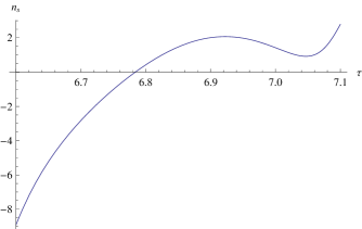
Figure 6: The scalar spectral index $n_{s}$ as a function of conformal time.

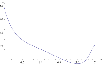
Figure 7: The running of the scalar spectral index $\alpha_{s}$ as a function of conformal time.

At $\tau\approx 7.05$ the spectral index is $n\approx 0.95$, and the running of the spectral index is $\alpha\approx 0.$ This is within the allowed value of WMAP constraints Komatsu:2010 .

Now, consider the tensor perturbation. The mismatch of the standard fit function is shown in Fig.$\left(5\right)$. The fit function $2/(\tau-7.4)^{2}$ is a good approximation in the asymptotic region. This is because the first slow-roll parameter is approaching zero when $\tau>6.$ Despite the success in the asymptotic region, the validity of Bunch-Davies boundary condition is questionable. The reason is that Bunch-Davies vacuum imposes a condition at a fictitious conformal time $\tau\rightarrow-\infty$, while in the physical universe actually starts its expansion at a finite conformal time $\tau\approx 0.92.$ The limit $\tau\rightarrow-\infty$ is inapplicable in our model thus the mode function evaluated from the evolution of such ,an ill defined boundary condition is not reliable. Thus, we shall keep the standard fit function but abandon the boundary condition that is imposed at an unphysical time. We will proceed by obtaining a general solution of the mode function, and then subsequently use the observational constraints to restrict the possible parameters. Since the power spectrum of tensor perturbations has yet to be observed, experimentally what we have to constrain is the ratio of tensor perturbation to the scalar perturbation.

The most general mode function for the tensor modes is

$$\mu_{k}\left(\tau\right) =a\sqrt{k\tau}H_{3/2}^{(1)}(k\tau)+b\sqrt{k\tau}H_{3/2}^{(2)}(k\tau)$$ (69)

$$=a\frac{e^{-ik\tau}}{\sqrt{2k}}\left(1-\frac{i}{k\tau}\right)+b\frac{e^{ik\tau}}{\sqrt{2k}}\left(1+\frac{i}{k\tau}\right)$$ (70)

From the definition $\left(\ref{tensor power}\right)$ one obtains

$$P_{h}=4\frac{H^{2}}{k^{3}}+8\frac{H^{2}}{k^{3}}\left(b_{0}^{2}-b_{0}\sqrt{1+b_{0}^{2}}\cos\left(\tilde{\bigtriangleup}\right)\right)$$ (71)

Together with P_R computed from Eq.$\left(\ref{scalar mode}\right)$ as well as the observational restriction on $r$, one can deduce an upper bound for $\left(2b_{0}^{2}-2b_{0}\sqrt{1+b_{0}^{2}}\cos\left(\tilde{\bigtriangleup}\right)\right).$ From the WMAP7 data Komatsu:2010 $r<0.2$, which corresponds to $\left(2b_{0}^{2}-2b_{0}\sqrt{1+b_{0}^{2}}\cos\left(\tilde{\bigtriangleup}\right)\right)<0.16.$

III.2 The General Case

We would like to comment on how to generalize this program, such that it may be implemented for a given background evolution of an inflationary model. There is no reason, a priori, that either Eq.$\left(\ref{standard fit}\right)$ in the standard method, or a quadratic function, as introduced in the previous section, should be a good fit for $z^{\prime\prime}/z$ in general.

Our proposal in this paper has been to point out that one should not apply the standard fit function to all inflationary models without carefully examining whether it is actually a good fit. If the analytic solution for the Mukahanov-Sasaki equation is not attainable, one may wish to find a fit function that is analytically solvable. There exist a number of analytically solvable fit functions for $z^{\prime\prime}/z$, the quadratic function introduced in the previous section is just one simple example.

Another more sophisticated example is the quartic function which renders Eq.$\left(\ref{Muk}\right)$ solvable by linear combinations of the Heun triconfluent function. Unfortunately in practice, the introduction of a more complicated fitting function, such as the quartic function, may reduce the predictivity of the model as there will tend to be more parameters in the fit function that require matching rules to pin down their values. However the rule of thumb is simple, the employed fit function should resemble the actual curve at the region of interest, which is the moment of horizon crossing. After that, one should impose the boundary condition at a meaningful time. As we have demonstrated, using the WKB approximation at the moment when $z^{\prime\prime}/z$ is flat is one sensible choice. Finally, one can use the current observational data for the tensor to scalar ratio to constrain tensor perturbation. However, since the power spectrum of the tensor mode has not been observed, the constraints from the tensor sector are not overly restrictive.

IV Conclusions

In order to make predictions testable by observations, inflation needs not only a model, but suitable boundary conditions. Some models of inflation do not seem to fall within the realm where the standard boundary conditions may be naturally applied. With this in mind, we have discussed the introduction of an alternative method which generalizes the standard approach of computing the scalar and tensor power spectra. It is suggests that for those models whose background is analytically solvable, one should re-examine their power spectrum using our method and find how does their spectral index compare with the results from standard method.

In general, this procedure will introduce additional parameters into the model, thus allowing more accurate phenomenology, with the usual drawback that introduction of more parameters decreases predictivity. This new method is implemented on a model-by-model basis, hence the generic effects of this approach have yet to be determined. For the specific example discussed in this paper, we explored an inflationary model which has analytically solvable background dynamics. We introduced a quadratic fit (of course, other models may require more complicated fitting functions)for the function $z^{\prime\prime}/z$ which appears in the Mukhanov-Sasaki equation for the scalar modes, and imposed boundary conditions at finite conformal time, $\tau$. It was found that near $\tau=7.05$ the spectral index and its running, both fall into a phenomenologically acceptable range. This calculation gives an example for the implementation of our approach, although the model in question is not fully realized in the sense that it lacks a proper accounting for the cessation of inflation in order to produce the requisite amount of e-fold expansion.

The capacity for altering the calculation, and thus the values, of observables predicted by inflation via this new approach is clear. It may therefore be possible that models which were hitherto discarded may need to be re-investigated in the framework of this method.

- (1) A. H. Guth, Phys. Rev. D 23, 347 (1981)
- (2) A. D. Linde, Phys. Lett. B 108, 389 (1982)
- (3) A. Albrecht, P. J. Steinhardt, Phys. Rev. Lett. 48, 1220 (1982)
- (4) L. A. Kofman and V. F. Mukhanov JETP Lett. 44 619 (1986)
- (5) M. Sasaki, Prog.Theor.Phys. 76 (1986)
- (6) T.S. Bunch and P.C.W. Davies, Proc. Roy. Soc. Ser. A 360, 117 (1978).
- (7) U. H. Danielsson, Phys. Rev. D 66 23511 (2002)
- (8) B. Green, K. Schalm, J. Pieter van der Schaar, G. Shiu. [astro-ph/0503458]
- (9) R. Easther, W.H. Kinney, and H. Peiris, JCAP 0508:001 (2005) [astro-ph/0505426].
- (10) X.Chen, M.-X. Huang, S. Kachru, and G. Shiu, JCAP 0701:002 (2007) [hep-th/0605045].
- (11) R. Holman and A.J. Tolley, JCAP 0805:001 (2008) [arXiv:0710.1302]
- (12) P.D. Meerburg, J.P. van der Schaar, and P.S. Corasaniti, JCAP 0905:018,2009 [arXiv:0901.4044]
- (13) L. Sriramkumar and T. Padmanabhan, Phys.Rev.D 71 103521 (2005) [gr-qc/0408034]
- (14) A. Ashoorioon and G. Shiu, arXiv:1012.3392 [astro-ph.CO].
- (15) N. Kaloper, M. Kleban, A. Lawrence, S. Shenker, L. Susskind, JHEP 0211:037 (2002)
- (16) E. D. Stewart and D. H. Lyth, Phys. Lett. B 302 171 (1993) [gr-qc/9302019].
- (17) S. Weinberg, Cosmology, Oxford University Press Inc., New York (2008). D. Baumann, TASI Lectures on Inflation [arXiv:0907.5424].
- (18) E. Komatsu et al. [arXiv:1001.4538].
- (19) L.P. Grishchuk, Class. Quant. Grav. 10 2449-2478, (1993) [gr-qc/9302036].
- (20) I. Bars and S. H. Chen, [arXiv:1004.0752]
- (21) R. Easther, Class. Quant. Grav. 10 2203, (1993) [gr-qc/9308010]
- (22) J. D. Barrow, Phys. Rev. D 48 1585 (1993)
- (23) J. D. Barrow, Phys. Rev. D 49 3055 (1994)
- (24) G.F.R. Ellis and M.S. Madsen, Class. Quant. Grav. 8 667 (1991)
- (25) J. E. Lidsey Class. Quant. Grav. 8 923 (1991)
- (26) R. Easther Class. Quant. Grav. 13 1775 (1996) [astro-ph/9511143]
- (27) J. P. Mimoso and T. Charters J.Phys.Conf.Ser. 229 012051 (2010)
- (28) M. Abramowitz and I.A. Stegun, Handbook of Mathematical Functions, Dover (1965), ISBN 0486612724.