Quantum deformation of two four-dimensional spin foam models
Abstract
We construct the q-deformed version of two four-dimensional spin foam models, the Euclidean and Lorentzian versions of the EPRL model. The q-deformed models are based on the representation theory of two copies of at a root of unity and on the quantum Lorentz group with a real deformation parameter. For both models we give a definition of the quantum EPRL intertwiners, study their convergence and braiding properties and construct an amplitude for the four-simplexes. We find that both of the resulting models are convergent.
1 Introduction
Background and motivation
Manifold invariants of representation theoretic origin such as the Reshetikhin-Turaev invariant [1] or the Turaev-Viro invariant [2] play an important role in mathematical physics. In particular, they are of interest to quantum gravity, where models of the Turaev-Viro type are known under the name of spin foam models. The basic principle in the construction of a dimensional spin foam model is to assign irreducible representations to the -simplexes of a triangulated manifold and intertwining operators to the -simplexes which intertwine the representations associated to their boundaries. Higher-dimensional simplexes in the triangulation are then decorated with representation theoretical data constructed from these representations and intertwiners, often referred to as “amplitudes” in the literature. After a summation over all such assignments of representations and intertwiners the product of the amplitudes assigned to each higher-dimensional simplex define a number, the partition function of the model. In some three- and higher-dimensional models, one can show that the partition function converges and is independent of the choice of the triangulation. It thus defines a manifold invariant.
Among the spin foam models in the literature, one distinguishes models which are based on the representation theory of Lie groups (in the following referred to as “classical models”) and models which are based on the representation theory of quantum groups. Compared to the classical models, the latter have several advantages. The most important one is that they exhibit an improved convergence behaviour. When the relevant quantum group is a -deformed universal enveloping algebra of a simple Lie algebra at a root of unity, its tilting modules form a non-degenerate finite semisimple spherical category [3, 4]. In the corresponding spin foam model, this has the effect of replacing infinite sums in the classical models by finite sums in the -deformed models.
In the case where is not a root of unity, the representation theory of the -deformed universal enveloping algebras is more complicated, but the associated spin foam models still often show an improved convergence behaviour compared to the classical ones. From the physics perspective, the -deformed models can be viewed as regularisations of the corresponding classical models. They remove divergences that occur when the representation labels grow large. Since these labels carry an interpretation in terms of lengths or areas of the simplicial complex, these divergences are often referred to as infrared.
Examples of this effect in three dimensions are the Turaev-Viro model [2], which is based on the tilting modules for at a root of unity. It can be viewed as a regularisation of the (divergent) Ponzano-Regge model [5], which is based on the representation theory of . A similar example in four dimensions is the relation between the Crane-Yetter model [6, 7] and the Ooguri model [8], which are based on the representation theory of, respectively, at a root of unity and . The former defines a topological invariant of -manifolds which can be expressed in terms of the signature and the Euler characteristic of the manifold [9].
Quantum groups also appear in constrained topological models of four-dimensional quantum gravity. The idea underlying the construction of such models is the fact that gravity in dimensions greater than three can be written as a constrained BF theory333The name BF theory stems from the letters and that were used for the field variables in the first formulation of the theory. [10]. Constrained topological models are an attempt of incorporating these constraints into a spin foam model by imposing appropriate restrictions on the representations and intertwiners that are assigned to the faces and tetrahedra of the triangulation.
The first such constrained topological model is the BC model due to Barrett and Crane [11, 12]. Similarly to the topological models, this model diverges for large values of the representation labels. Yetter [13] and Noui and Roche [14] constructed -deformed analogues of the Euclidean and Lorentzian versions of the model based on, respectively, the representation category of and . Both -deformed models exhibit enhanced convergence properties compared to their classical counterparts.
Recently, the implementation of the constraints reducing BF theory to gravity in 4d spin foam models was refined and improved. This led to the formulation of new constrained topological models by Engle, Pereira, Rovelli and Livine (EPRL) [15] and Freidel and Krasnov (FK) [16]. These models incorporate a free parameter , called the Immirzi parameter. The limits and yield respectively the BC and the flipped EPR model [17, 18, 19].
These recent models exhibit interesting physical properties, such as an asymptotic behaviour related to the Regge action [20, 21, 22, 23, 24, 25], but suffer from divergences for large area variables (see [26] for an analysis of these divergences). As originally suggested by Rovelli [27], this indicates the need for -deformed versions of these models, which still have the relevant physical properties but have a better chance of convergence. Furthermore, there is evidence that such models could be related to gravity with a positive cosmological constant. The construction of these models is the aim of this article.
Main results
In this article, we construct a -deformed version of both the Euclidean and Lorentzian EPRL model [15]. The formulation of the Lorentzian model uses techniques from the representation theory of non-compact quantum groups and applies them to the quantum Lorentz group with a real deformation parameter. Using the results by Buffenoir and Roche [28, 29] on the harmonic analysis of the quantum Lorentz group, we construct a generalisation of the integral definition of the classical EPRL intertwiner to the quantum Lorentz group by means of a Haar measure on the latter. This is followed by a detailed analysis of the properties of the resulting intertwiner, including a proof of its convergence. We also derive explicit expressions for its transformations under braiding, under which the quantum EPRL intertwiner turns out not to be invariant. We then define an amplitude for the -simplexes of a triangulated four-manifold and construct the associated quantum spin foam model. Remarkably, the model converges although it is based on representations of an infinite-dimensional Hopf algebra.
The Euclidean model is formulated in terms of representation categories rather than the language of Hopf algebras. This structural difference with the Lorentzian model is explained by the fact that the Euclidean model is based on the representation theory of (two copies of) at a root of unity. While the representation theory simplifies considerably in this case - the tilting modules [3, 4] of at a root of unity define a non-degenerate, finite semisimple spherical category- the corresponding Hopf algebra structures become complicated, and one is forced to enter the framework of weak, quasi-Hopf algebras. The -deformed generalisation of the Euclidean EPRL intertwiner is therefore formulated in terms of the representation theory of rather than in terms of Haar measures on Hopf algebras. In this case, there are no convergence issues since there is only a finite number of representations with non-vanishing -dimension. As in the Lorentzian case, the quantum EPRL intertwiner does not appear to be invariant under braiding. After our discussion of the EPRL intertwiner, we then define the amplitude for a four simplex in the resulting model and show that it factorises into two quantum symbols with fusion coefficients. This mirrors the behaviour of the amplitude in the classical Euclidean EPRL model [15]. The resulting -deformed spin foam model is again finite.
Outline of the paper
The paper is organised as follows. Section is dedicated to the construction of the Lorentzian model. We start by reviewing essential notions on the quantum Lorentz group, its representation theory and Harmonic analysis in Section 2.1. In Section 2.2 we show how the Lorentzian EPRL intertwiner can be generalised to the quantum Lorentz group by means of a Haar measure on the quantum Lorentz group. We then prove an important convergence theorem that ensures that the quantum EPRL intertwiner is well-defined and investigate its behaviour of under braiding. In Section 2.3 we define an amplitude for the four-simplexes of a closed oriented triangulated four-manifold. This definition is given via a graphical calculus defined by means of an invariant bilinear form on the representation spaces of the quantum Lorentz group. This naturally leads to the definition of the quantum spin foam model which is shown to converge for all triangulated manifolds.
In Section , we construct the -deformed EPRL model for Euclidean signature. We start by summarising the relevant aspects of the quantum group at a root of unity and of its representation theory in Section 3.1. In Section 3.1.3 we give a brief description of the “quantum rotation group” and its irreducible representations. This background is then used in the construction of the Euclidean quantum EPRL intertwiner in Section 3.2. We analyse the properties of this intertwiner and then define the associated four-simplex amplitude in Section 3.3. We conclude the discussion by proving that this amplitude factorises into a quantum symbol and that the associated spin foam model converges for all triangulated closed four-manifolds. Section contains a discussion of the physical interpretation and properties of the two -deformed EPRL models as well as our outlook and conclusions.
2 The Lorentzian model
2.1 The quantum Lorentz group
In this subsection, we summarise the relevant definitions and results about the quantum Lorentz group following [30, 28, 29]. The quantum Lorentz group is an infinite-dimensional ribbon Hopf algebra, which is obtained as the quantum double or Drinfel’d double of the -deformed universal enveloping algebra , where is a real deformation parameter.
2.1.1 Hopf algebra structure
The Hopf algebra .
We start by introducing the Hopf algebra , adopting the conventions from [28]. The star Hopf algebra is the associative algebra generated multiplicatively by the elements , , subject to the relations
| (1) |
The comultiplication, counit and antipode are given by
| (2) | |||||
| (3) | |||||
| (4) |
and the star structure takes the form
| (5) |
The star Hopf algebra is a ribbon algebra with universal -matrix
| (6) |
where is the -exponential:
| (7) |
The ribbon element is defined by the identity , where is the invertible element and denotes the multiplication map. The group-like element is given by
| (8) |
Representation theory of
The representation theory of with a deformation parameter closely resembles the representation theory of the Lie group . Irreducible finite-dimensional -representations are labelled by “spins” and by an additional parameter . In the following we will restrict attention to equivalence classes of unitarizable representations which are characterised by the condition . As in the case of the Lie group , the representation space of the irreducible representation is -dimensional. There exists an orthonormal basis of the complex vector space in which the generators act according to
| (9) |
where is defined as in (7). The fusion rules for the tensor products resemble the ones for the representations of . We have
| (10) |
where the isomorphism is given by the Clebsch-Gordan intertwining operators
| (11) |
As all multiplicities in (10) are equal to one, these intertwiners are unique up to normalisation. They are non-zero if and only if , and are non-negative integers. Their coefficients with respect to the bases are the Clebsch-Gordan coefficients
| (12) |
To fix the phase of the Clebsch-Gordan coefficients, we impose reality conditions
| (13) |
and we use Wigner’s convention to fix the remaining sign ambiguity. The Clebsch-Gordan coefficients satisfy numerous relations. In the following we will frequently use their first orthogonality property and permutation symmetry
| (14) |
In some parts of the paper, we will identify the representation spaces with their duals by means of an invariant bilinear form on . We denote by be the dual vector space of the representation space in (2.1.1) and by be the basis dual to the basis :
The antipode (4) associates to each representation on a representation on via
The representations and are equivalent. The equivalence is given by a bijective intertwiner . Its matrix elements and those of the dual map with respect to the bases , are defined by
| (15) |
Here and throughout the paper, we use Einstein summation convention: repeated upper and lower indices are summed over unless stated otherwise. A short calculation using expression (4) and (2.1.1) shows that the matrix elements of and its dual are given up to normalisation by
| (16) |
where the constant is fixed to and is given by the action of the ribbon element (645) on . The matrix elements satisfy the identities
| (17) |
The intertwiner defines an invariant bilinear form on the vector space via
| (18) |
The Hopf algebra .
The star Hopf algebra is the dual of the Hopf algebra and can be viewed as a quantum deformation of the algebra of polynomial functions on . A basis of is given by the matrix elements in the unitary irreducible representations (2.1.1) of
| (19) |
The pairing between and takes the form
| (20) |
The Hopf algebra structure of induced by the one on via the pairing (20). In terms of the matrix elements , its algebra structure is characterised by the relations
| (21) |
Its comultiplication, counit and antipode take the form
| (22) | ||||
| (23) | ||||
| (24) |
where is the Kronecker symbol for the representation labelled by and the coefficients are given by (16). The star structure is given by
| (25) |
As any irreducible representation of can be obtained by tensoring the fundamental representation labelled by , a set of multiplicative generators of is given by the matrix elements in the fundamental representation
They generate multiplicatively subject to the relations
| (26) | ||||||
In terms of these generators, the comultiplication, counit and antipode are given by
| (27) | ||||
| (28) | ||||
| (29) |
and the pairing takes the form
| (30) |
The quantum Lorentz group .
The quantum Lorentz group is the quantum double of . It is given as the star Hopf algebra
where is the Hopf algebra with opposite coproduct, and the symbol ‘’ indicates that the Hopf subalgebras and do not commute inside . The algebra structure is given by (1), (21) together with mixed relations, that are most easily given in terms of the multiplicative generators of , see for instance the appendix of [28]. In terms of these variables and the standard generators of they take the form
| (31) | ||||||
The comultiplication, counit and antipode for are given by equations (2), (3), (4) for the Hopf subalgebra and by the opposite of the comultiplication in (22), the counit in (23) and the inverse444The antipode of a Hopf algebra with the opposite coproduct is the inverse of the antipode of the Hopf algebra . of the antipode (24) for the Hopf subalgebra . The star structure is given by (5) and by (25), where the antipode in (25) is replaced by its inverse. As it is a quantum double, the quantum Lorentz group is a braided Hopf algebra. We will describe its universal -matrix after introducing its double dual in Section 2.1.2 below.
The quantum Lorentz group is a quantum deformation of the universal enveloping algebra of the real Lie algebra . This is a direct consequence of the quantum duality principle, see for instance [28, 31, 32, 33]. Recall that the coalgebra structure on the deformed enveloping algebra of a Lie algebra induces a Lie algebra structure of the dual vector space . The principle of quantum duality states that the -deformed universal enveloping algebra of is given by . On the level of quantised function spaces, one obtains that the Hopf algebra of quantum deformations of polynomial functions on the group is given by , where .
In the case at hand, this yields [28], where is the Lie algebra of the group . Here, denotes the group of diagonal positive -matrices of determinant one and is the nilpotent group of lower triangular two by two matrices with diagonal elements equal to one. The quantum double construction is therefore the quantum analogue of the Iwasawa decomposition of the classical Lorentz algebra , and we will use the notation .
2.1.2 Irreducible representations, duals and -matrix
Irreducible representations of the quantum Lorentz group
The irreducible unitary representations of were first classified by Pusz [34]. In this paper, we will only consider the representations of the principal series. These representations are labelled by a couple with and or with and . We denote by the representation of labelled by . It is a Harish-Chandra representation which decomposes into representations of as follows
| (32) |
where is the left -module (2.1.1). A basis of the infinite dimensional vector space is given by where, for fixed , is the basis of defined before equation (2.1.1). In terms of this basis, the action of on the representation space is given by equation (2.1.1) for the action of and the following action of
| (41) |
where are complex numbers defined in terms of analytic continuations of symbols for . As their expressions are lengthy and complicated, we will not give them here but refer the reader to [28], where they are derived explicitly, and to [29] where their properties are studied in depth.
By introducing a hermitian form for which the basis is orthonormal
the representation spaces can be given a pre-Hilbert space structure. Its completion with respect to the associated norm is separable Hilbert space with Hilbert basis . The representations of the principal series are unitary in the sense that for all in and for all in , , that is, .
Note that the finite-dimensional unitary representations of the quantum Lorentz group do not form a ribbon category. As the representation spaces are infinite-dimensional, there is no notion of (quantum) trace. As in the classical case, this poses a considerable obstacle for the definition of the amplitude for the four-simplexes of the EPRL model and the definition of a consistent graphical calculus for the quantum Lorentz group. We will come back to this point in the sequel.
Algebra of functions on the quantum Lorentz group.
Matrix elements of the principal representations of the quantum Lorentz group are linear forms on and hence elements of its dual . In the following, we will therefore consider the Hopf algebra of functions on the quantum Lorentz group. The algebra decomposes as [28], where the Hopf algebra is interpreted as the space of (compactly supported) functions on . It is the dual of the Hopf algebra and hence can be identified with the Hopf algebra with the opposite multiplication.
Denoting by the basis of introduced in (19) and by the elements of its dual basis given by
one finds that a convenient basis of is provided by the elements . The star Hopf algebra structure of follows immediately from the one of via the duality principle. In particular, one finds that the multiplication on takes the form
| (42) |
Universal -matrix and braiding.
To obtain a simple expression for the universal- matrix of , it is convenient to work with the Hopf algebra introduced in [28], which can be viewed as the double dual of . As the Hopf algebra is infinite-dimensional, this is not identical to but contains as a Hopf subalgebra [28]. It factorises as . A convenient basis of is given by the basis dual to . In terms of this basis, the universal -matrix of takes a particularly simple form, namely
| (43) |
To derive an explicit expression for the braiding, we note that if is a principal representation of on , there is a unique representation [28] of on , which will also be denoted by . Its action on the basis elements of the preHilbert space is given by
| (44) | |||||
| (53) |
where are the coefficients from (41). It is then immediate to obtain explicit expressions for the action of the universal -matrix in these representations:
| (54) |
where and . Note that although these sums are infinite, there is only a finite number of non-zero terms [29]. Consequently, there are no issues with convergence.
2.2 The quantum EPRL intertwiner
We are now ready to construct the generalised EPRL model associated with the quantum Lorentz group. The first step is to define the state space associated to the three-simplexes of a triangulated -manifold . This is the vector space of EPRL intertwiners between the four EPRL representations associated with its boundary triangles and the trivial EPRL representation on .
2.2.1 Quantum EPRL representations
A central ingredient in the construction is the generalisation of the notion of an EPRL representation to the quantum Lorentz group. In the classical model, an EPRL representation assigns a representation of to each finite-dimensional representation of . This assignment can be viewed as a lift from the representation category of to the representation category of , and is given by the prescription
where labels the irreducible representations of and is the Immirzi parameter. In the quantum Lorentz group, the -representations in the classical model correspond to irreducible representations of the Hopf algebra , which are labelled by a parameter . The inclusion , is replaced by the inclusion , . It is thus natural to require that that quantum EPRL representations are given by a tensor functor between the category of representations of and the representation category of the quantum Lorentz group, which is compatible with this inclusion of into . The image of the functor is a subset of representations of called EPRL representations. The analogy with the classical case suggests that this functor should act on the irreducible representations of according to
where labels an irreducible unitary principal series representation of the quantum Lorentz group and is the Immirzi parameter. Note, however, that the parameter in the representation labels of the principal series is restricted to the interval . To obtain a consistent definition, it is thus necessary to restrict the preimage of this functor, i. e. the representation label . Remark also that there is no loss of generality in considering only the case where is positive since the representations and are equivalent. We are now led to the following definition.
Definition 2.1.
(EPRL representations) Let be a fixed real positive parameter (the Immirzi parameter) and consider the subset of irreducible representations of labelled by
The Lorentzian EPRL representation of spin is the principal representation of labelled by
The restriction of the representation labels of to the label set ensures that the Lorentzian EPRL representation is a principal representation of the quantum Lorentz group, which would not be the case otherwise. It decomposes into irreducible representations of as follows
| (55) |
2.2.2 Quantum EPRL intertwiners
We are now ready to generalise the notion of quantum EPRL intertwiner to the quantum Lorentz group. This requires a generalisation of integral expressions of the type
| (56) |
where is a compact, unimodular Lie group with Haar measure , are unitary irreducible representations of and and . The generalisation of such integrals to -deformed universal enveloping algebras and the associated -deformed function spaces requires the notion of a Haar measure or biinvariant normalised integral on . This is a non-degenerate linear form that satisfies the identities
| (57) |
For a pedagogical introduction, see for instance [35]. The identities (57) imply that a Haar measure on is invariant under the left- and right-action of on . For given , the left- and right- action are defined via the pairing between and :
| (58) |
The invariance property (57) then implies
| (59) |
The Haar measure is thus invariant under the left- and right-action of the Hopf algebra on its dual , and this invariance can be viewed as a a generalisation of the left- and right-invariance of the Haar measure on a unimodular Lie group.
Given a Haar measure on , it is straightforward to generalise expression (56) to the representations of [29], [14]. For this, one introduces a basis of and denotes by the associated dual basis of . Given irreducible representations , , of , one obtains a representation of on the tensor product of the associated representation spaces
where denotes the -fold coproduct in : for , . The integral (56) then corresponds to the expression
| (60) |
Note, however, that the existence of a Haar measure on and the convergence of expression (60) is not guaranteed a priori in the case where and are infinite-dimensional.
In the case of the quantum Lorentz group, we consider the -deformed universal enveloping algebra and its dual . It is shown in [28, 29] that a Haar measure on is obtained from the decomposition introduced in Section 2.1.2. It is unique up to normalisation and given as the tensor product of the unique normalised biinvariant integral on and a right-invariant integral on . On the basis elements of and the basis elements of the latter take the form
| (61) |
The Haar measure on is therefore given by
| (62) |
where denotes the matrix elements of the group-like element in (8) in the representation labelled by
This reduces the summation over the basis in (60) to a summation over the parameters and . It is shown in [29] that the associated expression for in (60) converges for and defines an intertwining map .
This map allows us to generalise the notion of an EPRL intertwiner to the quantum Lorentz group. For this, we consider the projection , which maps the EPRL representation labelled by to the lowest weight factor in the decomposition (55) of . In terms of the basis of and the basis of , this projector takes the form
| (63) |
We will also make use of the inclusion maps associated to the the decomposition (55) which satisfy the identity . The dual of the projector defines an embedding of the vector space of linear forms on into the vector space of linear forms on . It defines one of the building blocks in the construction of an embedding
of the vector space of -valent ) intertwiners into the vector space of -valent intertwiners for the quantum Lorentz group. This embedding map will be noted . Given an element , we define the quantum EPRL intertwiner associated with as the image of under . This yields the following definition.
Definition 2.2.
(Quantum EPRL intertwiner) Let be a -tuple of elements of the label set and be the corresponding representation space of . Denote by the associated -tuple of EPRL representations and by the tensor product of their representation spaces. The quantum EPRL intertwiner associated to an intertwiner in is the linear map
| (64) |
where the map is given as the tensor product of the map (63)
| (65) |
As the definition of the EPRL intertwiner involves an infinite sum over basis elements of and their duals, it remains to show that the series in (64) converges for all choices of -intertwiners . For this, we introduce a basis of the vector space , which corresponds to the specification of a recoupling scheme. In the following we will mainly be interested in the case . In this case, an orthogonal basis of is given by the set of -intertwiners with
| (66) |
where is an element of , and , , denotes the evaluation in the ribbon category of representations of . This implies that the evaluation of the intertwiner is given in terms of Clebsch-Gordan coefficients as follows
| (77) |
Using the orthogonality of the Clebsch-Gordan intertwiners (14) and the properties of the map stated in (16), one obtains an orthogonality relation for the coefficients of the intertwiners
| (78) |
We can now demonstrate the convergence of the four-valent quantum EPRL intertwiners to elements of and obtain the following theorem.
Theorem 2.3.
Consider the -tuple of irreducible representations of associated with parameters in the label set and denote by the corresponding -tuple of EPRL representations. Let be an element of the basis of and a basis of . Then the evaluation of the quantum EPRL intertwiner is given by
| (95) | ||||
| (112) | ||||
| (121) |
This series converges absolutely and defines an element of .
Proof. The proof contains two steps. We first show the identity (2.3) and then prove the convergence. By definition, the evaluation of the EPRL intertwiner is given by the expression
where is a shorthand notation for , and we use Sweedler’s notation . We now choose as the basis of the basis with elements introduced in Section 2.1.2. Its dual is the basis of with basis elements . Using equation (44), we obtain
| (138) | |||
| (141) | |||
| (158) |
where we inserted the definition (63) of the -intertwiner to derive the second expression from the first. The next step is to compute the integrals and . This is done by use of the expressions (21), (42) for the multiplication on and , respectively, together with the definition of the integrals (663). This yields for the integral on
| (159) |
The Haar integral on is computed analogously. The first step is to derive the identity
| (168) | ||||
| (177) |
It is then easy to compute the bivalent integral
where we used the identity
to obtain
| (178) |
The expression for the evaluation of the EPRL intertwiner then takes the form
| (185) | ||||
| (202) | ||||
| (219) |
Using the orthogonality property (78) of the Clebsch-Gordan coefficients and simplifying the resulting expressions, we then obtain equation (2.3).
To prove the absolute convergence of the series, we bound the absolute value of the summands by the summands of a convergent series. We start be expressing (2.3) as
| (220) |
where is a function of the labels given by
and the summand takes the form
| (221) |
with
| (234) | |||
| (255) |
We can now bound the summand of the series as follows. Using the fact that the Clebsch-Gordan coefficients are bounded by one and the identity , we obtain
We then use the asymptotic properties of the coefficients which are derived in [29]. It is shown in [29] that there exist constants such that
| (256) |
This implies that for sufficiently large, , we have the following bound on the summands (221) of the series (220):
where is a constant and we have used the asymptotic identities and (256). As , the series converges for all and the series (220) converges absolutely. By using the left invariance of the Haar measure, one then finds that the quantum EPRL intertwiner is an element of .
To conclude our discussion of the quantum EPRL intertwiner, we investigate its transformation under braiding. As the following proposition shows, unlike the quantum Barrett-Crane intertwiner [14], the quantum EPRL intertwiner is not invariant under braiding. For simplicity, we will concentrate on the braiding of the two first arguments. The general case can be treated analogously.
Proposition 2.4.
Let , , be a -tuple of of irreducible representations of with associated EPRL representations . Consider the intertwiner for an element . Then the transformation of the EPRL intertwiner under the braiding of the first two EPRL representations is given by 555Note the abuse of notation in the right hand side of equation (257); is not necessarily an EPRL representation. The notation is used nevertheless for compacity purposes.
| (257) |
Proof. As the braiding is an intertwiner between the representations of the quantum Lorentz group on and , we have
where is the permutation that exchanges the first and second argument. Inserting expression (54) for the action of the -matrix on the principal representations into the definition of the braiding and using the definition (63) of the projector we obtain
| (266) | ||||
We now evaluate this expression by using identity (77) which expresses the intertwiner in terms of the Clebsch-Gordan coefficients. Due to the orthogonality of the Clebsch-Gordan maps (14), we can then recombine two coefficients and rewrite expression (266) as
| (267) | |||
| (276) | |||
| (279) | |||
This proves the claim.
2.3 The four-simplex amplitude
We are now ready to construct the amplitude for -simplexes labeled by EPRL representations and -EPRL intertwiners. Such an amplitude is defined with the aid of the graphical calculus of spin networks. There are two main difficulties in the definition of the amplitude that arise from the fact that the representation spaces of the EPRL representations are infinite-dimensional. The first is that there is no coevaluation map that intertwines the trivial representation of the quantum Lorentz group on with a representation on the tensor product and therefore no notion of a quantum trace. The second difficulty is that a naive definition of the amplitude for the four-simplexes gives an infinite answer.
These problems arise in a similar fashion in the classical Lorentzian BC [12] and EPRL [15] models. A solution to the first problem was provided in [22] where a Lorentzian graphical calculus based on non-invariant tensors and bilinear forms was invented. A regularisation prescription that circumvents the second difficulty has been given in [36] and [37] for the BC and EPRL models, respectively. Extending these procedures to the quantum Lorentz group, we will overcome these issues and consistently construct a finite amplitude for the -simplexes.
2.3.1 EPRL tensors and bilinear form on the representation spaces
We first need a notion of dual quantum EPRL intertwiners. These dual objects are required since we cannot pair -EPRL intertwiners together because of the absence of a coevaluation map. As in the Lie group case, the vector space does not contain tensors that are invariant under the action of the quantum Lorentz group and such objects do not exist per se. Accordingly, dual -EPRL intertwiners are replaced by non-invariant quantities which can be viewed as the quantum group analogue of the boosted intertwiners considered in [22]. These quantities, which are referred to as vertex functions in [14], will be called EPRL tensors in the following.
Definition 2.5.
(Quantum EPRL tensor) Let be a -tuple of representations of labelled by elements of . Denote by the associated -tuple of EPRL representations, and consider an element . The quantum EPRL tensor associated to is defined by
| (280) |
where is a basis of and is the dual basis of . The vector space of EPRL tensors associated with is the vector space , where denotes the space of linear maps from to .
The quantum EPRL tensors associated with the elements of the basis of will be denoted in the following.
To pair EPRL tensors together, we need a bilinear form on the representation spaces . This form is induced by an intertwiner between the representation spaces and their duals.
Lemma 2.6.
Let be the dual to the vector space . There exist a bijective intertwiner whose expression with respect to the basis of and the dual basis of is given by
| (281) |
where is a constant and is given by (16). The representations of the quantum Lorentz group on and are equivalent. The bilinear form
| (282) |
satisfies the invariance property for all .
Proof: We first show that the map is an intertwiner between the representation of the quantum Lorentz group on and on its dual . By definition, the latter is given by the antipode of the quantum Lorentz group
In terms of the basis defined after (42) and the bases and of and , the condition that defines an intertwiner takes the form
| (283) |
To prove this identity, we compute the matrix elements using (44). This yields
| (284) |
To compute the matrix elements of in , we use that the antipode is an anti-algebra morphism together with expression (22) for the antipode on . From the identification and the duality between and , it follows that the antipode on takes the form
| (285) | |||
From (44) we then obtain that its matrix elements are given by
| (294) | |||
| (303) |
where we used the definition of the -intertwiner given in (16) and the reality condition (13) on the Clebsch-Gordan coefficients. We can now rewrite the intertwining property (283) as
| (312) | |||||
| (321) |
This identity now follows by inserting the definition (281) of . Using (16) and the permutation symmetry (14) of the Clebsch-Gordan coefficients, we obtain for the first expression in (312)
| (330) | |||
| (339) | |||
| (348) |
Note that this expression vanishes unless in which case it reduces to
This coincides with the expression obtained by inserting (281) into the second expression in(312) for . Otherwise, the second expression in (312) vanishes. This proves that defines an intertwiner between the representations of the quantum Lorentz group on and on its dual . The second part of the lemma then follows directly from the definitions and from the intertwining property of .
In the following, we will set the constant to one for all .
2.3.2 Graphical calculus
We will now construct the four-simplex amplitude from EPRL tensors. To define the amplitude, it is convenient to use diagrammatic methods. More precisely, we will make use of the graphical calculus of spin networks. The idea behind this calculus is to organise tensor calculations according to a diagram drawn in the plane. To cover calculations based on the representation theory of the quantum Lorentz group, some constructions used routinely in the representation theory of finite-dimensional Hopf algebras do not work and the calculus is restricted to a certain class of diagrams. The elements needed for the construction of the four-simplex amplitude are as follows.
We denote by oriented dashed lines irreducible representations of and by oriented solid lines EPRL representations. The tensor product of representations is depicted by drawing the lines next to each other from the left to the right. The Clebsch-Gordan maps for are depicted by three-valent vertices involving three dashed lines as shown in Figure 1 a). The inclusion map is depicted by a black box as shown in Figure 1 b). We choose the conventions that diagrams are evaluated from bottom to top.
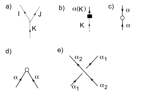
a) Clebsch-Gordan intertwiner for .
b) Inclusion map .
c) Intertwiner .
d) Bilinear form .
e) Braiding .
With this notation, it follows that the diagram for a EPRL tensor is given by Figure 2 a) and the one for an EPRL intertwiner by Figure 2 c). To keep the diagrams simple, we also introduce a shorthand notation, in which a EPRL tensor is depicted by a solid vertex with four ‘legs’ pointing upwards, away from the vertex as shown in Figure 2 b). The vertex is decorated with a cilium (short dashed line in Figure 2 b)) that indicates in which order the representations are coupled to the trivial representation. This cilium is labelled by the intermediate -representation as shown in Figure 2 b). The picture for an EPRL intertwiner is obtained by rotating the one for an EPRL tensor by 180 degree and inverting the orientation of the edges as shown in Figure 2 c),d).
To each vertex we associate a basis element of , which is omitted in the diagrams for reasons of legibility. The diagram for the tensor product of EPRL tensors is obtained by placing the vertices on a horizontal line, in the order in which they appear in the tensor product read from left to right.

a) EPRL tensor , b) Short notation for the EPRL tensor .
c) EPRL intertwiner , d) Short notation for the EPRL intertwiner .
EPRL tensors can be paired using the invariant bilinear form defined in equation (282). In the diagrams, this bilinear form is depicted by a white circle with two legs, one to the left, one to the right and both pointing towards the vertex, as shown in Figure 1 d). The precise details of the pairing are organised with the aid of the diagrammatic method. As the order of the two arguments of the bilinear form is important, the convention is that the first argument corresponds to the element on the left-hand side and the second argument to the right-hand side of the circle.
When more than one pair of edges are paired in a diagram, crossings can occur in the diagrams. To each such crossing we associate a braiding , where is the -matrix of the quantum Lorentz group defined in (43). Again, the precise form of the crossing is important and the braiding will be associated to the crossing where the left-hand leg goes under the right-hand leg as shown in Figure 1 e).
The diagrams are composed horizontally by tensor product, and vertically by the composition of maps. In this context, a vertical line corresponds to the identity map on a representation space . Note, however, that in contrast to the diagrams for ribbon categories, the upward and downward arcs have no direct meaning. The rules are that lines go upwards the EPRL tensors and can only be paired by the bilinear form , but they are free to go up and down between the vertices.
An important class of diagrams are closed diagrams. A closed diagram consists of a set of vertices arranged in a horizontal line, composed with crossings, vertical lines and pairings, in such a way that there are no free ends. A closed diagram corresponds to an element of . The evaluation of a closed diagram is then defined via the Haar integral in the spirit of Feynman diagram evaluations.
The naive evaluation of a closed diagram with vertices would correspond to setting . However, such an evaluation is generically divergent for the Lorentzian model and needs to be regularised. This is done in analogy to the classical case [36, 37] by removing the Haar measure or integration at one (randomly chosen) vertex as in [14]. The invariance of the Haar integral implies that the result is independent of the chosen vertex. Moreover, it implies that , where is a complex number or infinity and 1 is the unit in . As we will show in the following, if is the complete graph with five vertices, is finite, i. e. the diagram is integrable. The evaluation of is therefore obtained by applying copies of the Haar measure to and then applying the counit of to the resulting expression
2.3.3 Amplitude for the -simplexes
Let be an oriented, closed triangulated -manifold with sets of -simplexes . Consider a -simplex of . The set of tetrahedra of will be parametrised by , . Consequently, the triangles of will be labelled by ordered pairs , with . Let denote the braided tensor category of representations of the quantum Lorentz group.
Definition 2.7.
(Colouring) A colouring associates an EPRL representation of to each oriented triangle in .
From the colourings, one can construct state spaces for each tetrahedron of . The construction records the orientation of each tetrahedron in the boundary of
Definition 2.8.
(State space) Let denote a colouring. The state space associated with a tetrahedron appearing with positive sign in is read out of the colouring of its boundary and is defined by
Likewise, the state space for negative tetrahedra is given by
A state is an assignment of a EPRL tensor in either or to each tetrahedron in .
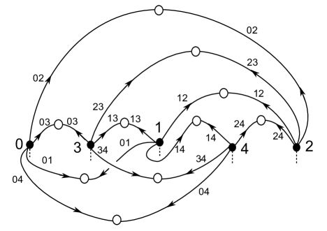
We are now ready to define the amplitude, or partition function, for the -simplex , which is given by the evaluation of the diagram in Figure 3.
Definition 2.9.
(-simplex amplitude) Let denote a colouring and a state. The amplitude for the -simplex is a linear map
obtained by evaluating the spin network diagram in Figure 3: .
We will now prove that the evaluation of this diagram is well-defined, i. e. that the four-simplex amplitude converges.
Theorem 2.10.
The four-simplex amplitude defined in Definition 2.9 converges absolutely.
Proof.
To prove this theorem, we consider the diagram depicted in Figure 4. The elements of the diagrammatic calculus are EPRL tensors, bilinear forms and braidings as explained in the previous subsection. At each vertex, we place an EPRL tensor , ,
To each line connecting two vertices we associate the bilinear form . This implies that each line coloured by carries a propagator, i.e., an element of given by
| (349) |
Note that the propagator is given by , where is the linear form on defined by
The diagram also contains a crossing to which we associate the braiding , given by . Throughout this proof, we will use the notation for the -matrix.
To simplify the notation, we label the lines of the diagram with numbers instead of associating labels to the vertices. The endpoints of each line carry a basis element of and our conventions are such that the left hand side of the line carries the basis element while the right hand side is coloured by the basis element . With the choice of cilium depicted in Figure 4, the element of associated to is thus given by
| (356) | ||||
| (361) | ||||
| (362) |
The next step is to calculate the propagators. This is achieved via a choice of basis, the elements of which are given by and . In this basis, the propagator takes the form
| (371) | ||||
| (372) |
where we used the definition of the antipode and the multiplicative structure of . With expression (44) for the representation and the explicit form of the bilinear form , we obtain
| (373) | ||||
| (390) |
We can now compute the propagators associated to the lines involved in the crossing. Denoting the -matrix by , we find that the first propagator is of the form
| (391) |
Using again the definition of the antipode and the product for , we obtain
| (396) | |||
| (417) |
The propagator associated to the second line in the crossing is given by
| (418) |
and after some further computations, we find
| (423) | ||||
| (436) |
We have thus derived explicit expressions for all quantities arising in (356) in terms of the Clebsch-Gordan coefficients for , the quantities from (41), the intertwiners (17) and the ribbon element for . It remains to evaluate the Haar integrals associated with the diagram. For this we need to select one of the five vertices that does not carry a Haar integral. In the following, we suppose that this vertex is the second vertex from the left in Figure 3. The amplitude associated to the diagram is then given by
| (437) |
The Haar integrals act on the basis elements and according to formulae (159) and (178). The counit is a morphism of algebras which acts on the basis elements according to
Combining these results, we find that the evaluation is given by an expression of the form
| (438) | ||||
where is a function of the representation labels that factorises as
| (439) |
The quantity depends only on the representation labels , which are fixed. The sums over the associated labels , , , for the basis elements of ,…, are thus finite. The quantities which depend on the summation indices , , in the sum (438) are contained in the function , which is given explicitly by
| (448) | |||
| (465) | |||
| (482) | |||
| (499) | |||
| (516) | |||
| (533) | |||
| (550) | |||
| (567) | |||
| (584) | |||
| (601) | |||
| (618) | |||
| (619) |
Implementing the delta functions in the above expression enforces the relations . Together with the Clebsch-Gordan conditions and the remaining delta functions, the conditions imply ; ; ; , and . This removes the sum over the representation labels in (619).
The resulting expression for is of the type obtained in the -deformation [14] of the Barrett-Crane model and can be represented by a spin network. The only difference is that our expression for involves contributions from the -matrix666Note however that the summation label arising from the expression of the -matrix is fixed to . and that, in contrast to [14], our spin network diagram contains open edges labelled with the variables . We can therefore follow the procedure in [14] and recouple the diagram to the product of an open diagram with a product of symbols. The open diagram depends only on the variables . It therefore contains only finite sums and is finite. The symbols for are bounded by one. We therefore find that the function is bounded by a polynomial in the variables . This implies that the evaluation (438) of the diagram is given by
| (620) | ||||
where the absolute values of the summands are bounded as follows
Moreover, it follows from the expression (619) that the function vanishes unless the representation labels in satisfy the following inequalities
| (621) | |||||
The first three inequalities in (621) imply that for fixed , the summation range of the variables and in (620) is restricted to finite intervals. We now take into account the asymptotic behaviour of the expressions and derived in [29]
| (622) |
where is a constant. For sufficiently large and , subject to the first three conditions in (621), we can thus bound the value of the summand in (620) by
| (623) | ||||
where is a polynomial in the variables that depends on the external parameters . As , this implies that there exists a constant such that
for all . The series in (620) then converge absolutely, because we have
| (624) | |||
and the series in the last expression reduce to finite sums due to the first three inequalities in (621). This proves the claim. ∎
2.4 The quantum spin foam model
Using the definitions and results from the previous subsections, we can now define the quantum EPRL spin foam model.
Definition 2.11.
Let be a closed oriented triangulated -manifold with sets of -simplexes . Let be a simplex of and let and denote its set of triangles and tetrahedra respectively. Let denote the corresponding EPRL-colouring, the associated EPRL-state, and let the 4-simplex amplitudes be given by Definition 3.6. The partition function for the quantum EPRL model associated to is given by
| (625) |
Here, the sum ranges over all in and over the elements of a basis of -intertwiners entering the definition of the EPRL tensors for each tetrahedron of . The state for the -simplex is given by , where is the state associated to the tetrahedron and the order in the tensor product is the one given in Definition 3.6. The products run over all the triangles and -simplexes of .
The weight associated to the triangles is fixed from gluing arguments as in the classical case [38]. As there is only a finite number of representations in the label set , the sum in Def. 2.11 involves only a finite number of terms and hence converges. Given the convergence of the EPRL intertwiners and the -simplex amplitude for fixed labels , the convergence of the Lorentzian -EPRL model is therefore immediate. However, the proofs of the convergence of the EPRL intertwiners and the -simplex amplitude in the previous subsection are intricate and require a careful analysis of the representation theory of the quantum Lorentz group.
3 The Euclidean model
In this section we study the Euclidean formulation of the model which is based on the representation theory of the quantum group at a root of unity. In this case, the generalisation of the EPRL-model is simple and more direct because it can be achieved in the framework of modular categories. These categories have been studied extensively and all ingredients needed in the construction of the model are available in the literature. The resulting model does not present the difficulties associated with the Lorentzian case. This is due to the fact that there is only a finite number of irreducible representations and, consequently, no risks of divergences.
3.1 The quantum rotation group
3.1.1 at root of unity.
We start with a brief summary of the representation theory of the Hopf algebra at a root of unity. In the following, we suppose that is a primitive th root of unity with odd. The Hopf algebra at a root of unity is most easily presented in terms of four generators that are given in terms of the generators in Section 2.1.1 by
| (626) |
The algebra structure and coalgebra structure are given by this identification together with formulas (1) to (4). However, the star structure differs from the one in Section 2.1.1 and takes the form
| (627) |
The finite-dimensional star Hopf algebra is the quotient of the Hopf subalgebra generated by by the two sided ideal generated by the elements . It can be identified with the associative algebra generated by subject to the algebra relations derived from (1) and the additional relations
| (628) |
Note that the star Hopf algebra is a ribbon Hopf algebra with universal -matrix
| (629) |
where and are defined as in (7). The ribbon element is defined by the relation with , and the group-like element takes the form .
3.1.2 Representation theory of at a root of unity
The representation theory of differs from the generic case and the classical case in two fundamental ways. Firstly, up to isomorphisms, there is only a finite number of irreducible representations. Secondly, has finite-dimensional indecomposable representations777An indecomposable representation has dimension and is characterised by a half-integer such that , see for instance [3, 4, 39, 40] or [32]. [39, 40], which are not fully reducible and have vanishing quantum dimension. As the tensor product decomposition of two irreducible representations contains indecomposable representations, the representations of do not form a fusion category.
This obstacle is overcome with the tilting module construction [3, 4], for a pedagogical introduction see [32]. In this construction the tensor product of the finite-dimensional irreducible representations is modified in a consistent way such that all factors arising in the tensor product decomposition of finite-dimensional irreducible representations are again finite-dimensional irreducible representations. The result is a modular category . As this category has been discussed extensively in the literature, see for instance [41], we limit our presentation to a brief summary that emphasises the link with the classical theory and the Lorentzian model.
Monoidal structure
We start by outlining its structure as -linear tensor category. The objects of are certain finite-dimensional irreducible representations of over , the tilting modules. Its morphisms are intertwiners between tilting modules. The category is a strict -linear monoidal category. This means that there is a -bilinear functor , which corresponds to the tensor product of representations, and a unit object , such that for all objects . The unit object corresponds to the representation of on that is defined by the counit .
Semisimplicity
The category is abelian, finite and semisimple. This implies that there is a finite collection of simple objects of , which correspond to finite-dimensional irreducible tilting modules and which are unique up to isomorphism. These simple objects are labelled by a half-integer with . Again, the representation spaces are -dimensional, and we denote by the orthonormal basis of . Then the action of the generators on takes the form
| (630) | ||||
Every object in is given as a direct sum of simple objects
| (631) |
and the tensor product of two simple objects decomposes into a direct sum of simple objects according to
| (632) |
Note that the decomposition is very similar to the one for generic . The only difference is that the tensor product decomposition is cut off at instead of continuing to if . The isomorphism in (10) is given by the Clebsch-Gordan morphisms , . As in the generic case, the vector space of intertwiners between and is either one-dimensional or trivial and the Clebsch-Gordan intertwiners are therefore unique up to normalisation. Their matrix elements with respect to the bases are the Clebsch-Gordan coefficients. They satisfy the same relations as in the generic case with the additional condition that they vanish unless
| (633) |
This condition implements the cut off in the fusion rules (632).
Braiding
Pivotal structure and duals
The category is a braided monoidal category with duals. This means that for each object of there is a dual object , which corresponds to the representation of on the dual vector space . It is given by the antipode
Moreover, for each object there are morphisms , the evaluation, and , the coevaluation, which satisfy the identities
| (643) |
The evaluation corresponds to the pairing between the vector space and its dual. In terms of the basis and the dual basis of , the evaluation and coevaluation are given by
They associate to each intertwiner between representations and a dual intertwiner from to given by
| (644) |
Note that due to the identity for all , the functor is not the identity functor.
Ribbon structure and quantum trace
The category is a ribbon category and thus equipped with a twist. The twist is given as a collection of self-intertwiners for each object , which commute with all morphisms. It is defined by the action of the ribbon element of . For simple objects it takes the form
| (645) |
The ribbon element and the related element define the quantum trace of the category , which is given as a collection of linear maps from the endomorphism space of each object to . It defines a non-degenerate pairing , . and is given by
| (646) |
The quantum dimension is defined as the quantum trace of the identity endomorphism . This implies in particular that the quantum dimension of the simple objects is given by .
Identification of objects and their duals
To exhibit the structural similarities between the Lorentzian and the Euclidean model, it will be useful to introduce an identification between each object and its dual . This amounts to a choice of basis for each representation space . By assigning the dual basis to the representation space , one obtains bijective intertwiners , . For irreducible objects their matrix elements with respect to the bases and take the same form as for a real deformation parameter
| (647) |
where is given by the ribbon element (645): . The matrix elements satisfy
| (648) |
Composing the intertwiner with the coevaluation yields a bilinear form on each representation space , which is invariant
For the simple objects , its expression in terms of the basis reads
| (649) |
3.1.3 Quantum .
In this section, we define the Hopf algebra that we will consider as the quantum counterpart of the Euclidean isometry group . As in the previous section, we fix the parameter to an odd primitive of unity .
The self-dual and anti-self-dual factorisation of the classical Lie algebra suggests a two parameter deformation , where is the deformation parameter for the first copy of and the one for the second copy. In the following, we will be interested in one parameter deformation which arises by specialising888Note that the construction differs from that of the quantum Barrett-Crane model [13] where . to . In other words, we consider as the the quantum version of the Lie group the ribbon star Hopf algebra . The multiplication, unit, coproduct, counit, antipode, -matrix and ribbon element on are inherited from the corresponding structures on
| (650) | |||||
| (651) | |||||
| (652) | |||||
where the flip map acts on the second and third copy of the four-fold tensor product , i.e., . Note that the two copies of commute.
The finite-dimensional representations of are obtained by tensoring pairs of finite-dimensional representations of . In the following, we will restrict attention to those representations which are obtained by tensoring two finite-dimensional irreducible tilting modules of . We denote the associated modular category by . The irreducible objects of are labelled by a couple of spins , each corresponding to a finite-dimensional tilting module. A basis of the module labelled by is given by . The action of on this basis takes the form
| (653) |
By tensoring two copies of the bilinear form (649), one obtains a bilinear form on which is invariant under this action. Moreover, due to the fusion rules (10) of the irreducible tilting modules, there is a well defined action of on each -module in (632), which is given by
This action is non-trivial that provided and satisfy the constraint (633).
3.2 The quantum EPRL intertwiner
We are now ready to construct the associated quantum EPRL-model. We start by defining the EPRL-representations. The construction is analogous to the Lorentzian case. The only difference is that in order to ensure that these representations are associated with objects of , we need to restrict the value of the Immirzi parameter to the interval and to impose that it is rational with . The case will be treated elsewhere.
Definition 3.1.
(EPRL representations)
Let be a fixed real parameter satisfying and . Let be the label set of simple objects in for which . Given an element , the associated Euclidean EPRL representation is the object with , with
| (654) |
Note that for a given , the constraints and on the Immirzi parameter ensure that the Euclidean EPRL representation labelled by decomposes into irreducibles
| (655) |
We denote by the tensor basis of : , and by the projection map associated to (655) that projects onto the highest weight factor in the decomposition (655). As in the Lorentzian case, we denote by the associated inclusion map defined by the identity . The projection map commutes with the action of and is given by the Clebsch-Gordan morphisms. In terms of the bases introduced above, it reads
| (656) |
To define the EPRL intertwiner, we need to specify the quantum counterpart of the expression
| (657) |
In contrast to the Lorentzian situation, this will not be achieved by using a Haar measure on the dual Hopf algebra of . The reason is that, in contrast to the situation for generic , there is no direct characterisation of the dual Hopf algebra of in terms of matrix elements of irreducible representations. A simple dimension-counting argument shows that the the matrix elements in the representations (630) do not form a basis of the dual Hopf algebra . A Poincaré-Birkhoff-Witt basis for is given by , which implies that the dimension of the vector space is . The matrix elements with respect to the representations (630) are linear functions on and hence elements of . However, the number of matrix elements obtained from the representations (630) is
The matrix elements with respect to the representations (630) therefore span only a proper linear subspace of and do not form a basis of the vector space . Although it is immediate to obtain an expression that has the appropriate invariance properties by setting , this is not sufficient to characterise a Haar measure on .
However, due to the fact that is a modular tensor category, there is an alternative generalisation of the classical expression (657) which makes use of the semisimplicity, for a pedagogical explanation see [42]. The fact that is a modular tensor category implies that for each object there is a unique endomorphism which can be expressed as
| (658) |
where labels a basis of intertwiners in , runs over the basis elements of and . For simple objects , the space of morphisms is trivial unless . The associated endomorphism therefore takes the form . For a general object the associated endomorphism is obtained by expressing as a direct sum of simple objects . In particular, this implies that for two simple objects , the morphism takes the form
The corresponding expression for general tensor products of irreducibles is obtained by consecutively coupling them to zero via the Clebsch-Gordan coefficients. Consequently, the endomorphism can be viewed as the counterpart of the classical expression (657) and expression (60) for the quantum Lorentz group. It generalises expression (657) to the category and allows us to define the quantum EPRL intertwiner.
Definition 3.2.
(Quantum EPRL intertwiner) Let be a -tuple of irreducible representations in and the corresponding representation space. Denote by the associated EPRL-representations defined as in (654) and by the tensor product of their representation spaces
Then the the quantum EPRL intertwiner associated to an element is the morphism defined by
| (659) |
where is given in terms of the morphism (656) by
Note that, unlike the Euclidean quantum BC intertwiner [13], the Euclidean EPRL intertwiner is not invariant under braiding. This follows directly from its definition in analogy to the Lorentzian case.
In the classical Euclidean EPRL model, it is possible to perform the Haar integrals in the definition of the EPRL intertwiner. This leads to a factorisation of the amplitude for the -simplexes in terms of -symbols. The next proposition gives the equivalent of this construction for the -deformed Euclidean EPRL model.
Proposition 3.3.
Let be the representation label of an EPRL representation. Then the associated EPRL intertwiner can be expressed as
| (660) |
where , and is given in the proof below.
Proof. We use the identity for any irreducible representation together with the complete reducibility of the tensor product of -modules
| (661) |
where , and are the Clebsch-Gordan maps for the representations of . They factorise into Clebsch-Gordan maps for the irreducible tilting modules of : for , . From identity (661), we then obtain
| (662) |
where is defined as and . With this result, it is immediate to compute for four-valent tensor products , which appear in the definition of the EPRL intertwiner. The computation proceeds as in the classical case. For , is given as a sum over the representation appearing in the intermediate channel of three-valent decomposition of a -valent intertwiner
| (663) | ||||
where is the evaluation map and is the morphism dual to . The intertwiner factorises into intertwiners of -modules according to
where is the appropriate flip map and
| (664) |
The evaluation of in our basis then yields
with
| (665) |
in analogy with previous results obtained for the Lorentzian model. Using this expression, it is then immediate to obtain the evaluation of and to express the quantum EPRL intertwiner as
| (666) | |||
To exhibit explicitly the structural similarities with the Lorentzian case, we construct the EPRL model for by making use of EPRL tensors, which are elements of . The main difference with respect to the Lorentzian model is that in the Euclidean case, the vector space is not-trivial. Therefore, EPRL tensors are bona fide intertwiners and are defined simply as the intertwiners dual to the EPRL intertwiners in Def. 3.2.
3.3 Four-simplex amplitude and the quantum spin foam model
We will now show how the amplitude for the four-simplexes can be defined for the Euclidean model. As the relevant representations form a modular category, there are no problems related to divergences and no regularisation is required. We start by defining the colouring and state space of a tetrahedron in analogy to the Lorentzian case. We again suppose that is an oriented, closed triangulated -manifold with sets of simplexes . Consider a -simplex of . We parametrise the set of tetrahedra of as in Section 2.3.3.
Definition 3.4.
(Colouring) A colouring associates an EPRL representation of to each oriented triangle in .
The state spaces for the tetrahedra are constructed from the colourings similarly to the Lorentzian case. The only difference is that in the Euclidean case, there is no need to implement the state space as a space of Hopf-algebra valued linear maps. Instead, we identify it with the space of intertwiners between the trivial representation and the tensor product of the EPRL representations at their boundary triangles.
Definition 3.5.
(State space) Let denote a colouring. The state space associated with a tetrahedron that appears with positive sign in is read out of the colouring of its boundary and is defined by
Likewise, the state space for negatively oriented tetrahedra is given by
A state is an assignment of an EPRL tensor in either or to each tetrahedron in .
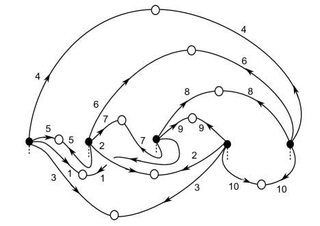
We are now ready to define the amplitude, or partition function, for the -simplex . This is done by the same diagrammatic method as in the Lorentzian case.
Definition 3.6.
(-simplex amplitude) Let denote a colouring and a state. The amplitude for a -simplex is the linear map
obtained by evaluating the spin network diagram in Figure 3 corresponding to the complete graph with five vertices , that is, .
The only difference to the Lorentzian case is the evaluation of the diagram. In the Euclidean case, there is no need to regularise the evaluation and is defined by the quantity that corresponds to in the Lorentzian case. The diagrammatic calculus is defined in the same way as in the Lorentzian section. However, the vertices of the diagram are now labelled by Euclidean quantum EPRL tensors, the lines are connected via the invariant bilinear form
and the crossing diagram corresponds to the braiding obtained by tensoring two copies of the braiding (3.1.2) of the category . Using these structures associated with the diagram components, one can then compute the quantity with depicted in Figure 3. The computation is analogous to the Lorentzian case, but all series arising there are replaced by finite sums. The amplitude therefore converges without further regularisation.
Using the factorisation of the quantum EPRL intertwiner in Def. 3.3, one can express the amplitude for the four-simplexes in terms of quantum symbols999Note that the notion of symbol used here is closely related to but not equivalent to the standard definition. The standard symbol is obtained by composing five Clebsch-Gordan morphisms for and closing the resulting expression with a quantum trace. As it is our aim to explicitly exhibit the similarities with the Lorentzian model, we work with a different expression, which is the analogue of the quantities called symbols there and in the classical EPRL models. for .
Definition 3.7.
(Quantum symbol) Let be a colouring and a state constructed from the representation theory of . The quantum symbol is defined as The quantum symbol for is the product of the -symbols for the two copies of
Using this definition, it is immediate to prove the following proposition.
Proposition 3.8.
The amplitude for the -simplex can be expressed in terms of a quantum symbol for as follows
where we use the shorthand notations , , and the intertwiners and the constants are defined in proposition 3.3.
This proposition shows that the amplitude for the -simplexes factorises in a way that is directly analogous to the classical case. Note that such factorisation would also occur in the Lorentzian model if one did not remove one of the Haar measures at the five vertices. In physical terms, the removal of one Haar measure amounts to a gauge fixing, which ensures the convergence of the model but breaks its symmetry. Without this gauge fixing, one would obtain a divergent expression for the amplitude that factorises formally into symbols.
Using the definitions introduced in the previous section, we can now define the quantum EPRL spin foam model.
Definition 3.9.
Let be a closed oriented triangulated -manifold with sets of -simplexes . Choose a fixed linear order of the vertices of . Let be a simplex of and let and denote its set of triangles and tetrahedra respectively. Let denote the corresponding EPRL-colouring, the associated EPRL-state, and let the 4-simplex amplitudes be given by Definition 3.6. The partition function for the quantum EPRL model associated to is given by
| (667) |
Here, the sum ranges over all in and over the elements of a basis of -intertwiners entering the definition of the EPRL tensors for each tetrahedron of . The state for the -simplex is given by , where is the state associated to the tetrahedron and the order in the tensor product is the one given in Definition 3.6. Finally, the product is over all the triangles and -simplexes of .
As an immediate consequence of the definition of the model we obtain that the partition function converges. This follows directly from the fact that the label set contains only a finite number of representations. Consequently, the expression for involves only a finite sums and hence does not exhibit any of the convergence issues associated with the classical models.
4 Discussion and conclusions
Summary
In this paper, we construct the -deformed spin foam models corresponding to the Lorentzian and Euclidean EPRL models. In the first part of the paper, we concentrate on the Lorentzian model. We review the construction of the quantum Lorentz group as the quantum double of together with its harmonic analysis given in [28, 29]. Using these results, we generalise the Lorentzian EPRL intertwiner to the quantum Lorentz group by means of a Haar measure. We prove that the quantum EPRL intertwiner converges and show that, in contrast to the intertwiners arising in the BC model [11, 12], it is not invariant under braiding. We then provide a consistent definition of an amplitude for the four-simplexes using a graphical calculus for the braided category of representations of the quantum Lorentz group. The resulting spin foam model for a compact triangulated four-manifold converges.
In the Euclidean case, we employ different methods to generalise the Euclidean EPRL intertwiner. Using the language of categories, we provide a generalisation of the classical intertwiner to the modular category of representations of at root of unity, obtained via the tilting module construction. The resulting intertwiner converges trivially and is also not invariant under braiding. We then define an amplitude for the four-simplexes analogously to the Lorentzian model by using the appropriate graphical calculus. As a result, we obtain that the amplitude can be expressed in terms of quantum symbols and fusion coefficients. As it only involves only sums over a finite set of representation labels, the resulting spin foam model converges.
Physical interpretation
Due to their convergence properties, -deformed spin foam models can be viewed as infra-red regularisations of the corresponding classical models. The divergences in the classical models associated with large values of the representation labels disappear as there is a cut-off which eliminates these representations. This cut-off on the representation labels can be interpreted as the presence of a horizon and appears to be related to the cosmological constant.
The correspondence between -deformations and the cosmological constant is well-known and understood in detail in the three-dimensional case. In three dimensions, the Turaev-Viro invariant is related to Euclidean gravity with a positive cosmological constant. This relation can be inferred from two perspectives. The first one is the investigation of the semi-classical limit of the model via the asymptotics of the amplitude for the three-simplexes (given by a quantum symbol). This limit involves the physical regime where the spins are bounded from below by the Planck length and from above by the cosmological length that corresponds to the de-Sitter horizon. The asymptotics of the quantum symbol has been computed in [43] and yields the cosine of the Regge action with a cosmological term.
An alternative way to relate the Turaev-Viro model to three-dimensional gravity with positive cosmological constant is obtained from the correspondence between three-dimensional gravity, BF theory and Chern-Simons gauge theory. Three-dimensional gravity with Euclidean signature and positive cosmological constant can either be expressed as a BF theory with cosmological constant or in terms of two -Chern-Simons actions [44] with level . As a result, the partition function of a three-dimensional BF theory with cosmological term defined on a three-manifold is equal to the modulus square of the partition function of Chern-Simons theory on : . On the other hand, it was shown by Witten [45] that the amplitude for a Chern-Simons theory on is equal to the Reshetikhin-Turaev [1] invariant for and . The fact that the Turaev-Viro sum of a manifold is equal to the modulus square of the Reshetikhin-Turaev invariant of , relates the Turaev-Viro state sum to BF theory with a positive cosmological constant:
| (668) |
By reintroducing natural units, one then finds that the deformation parameter of the Turaev-Viro model is related to the cosmological constant through the relation .
In four dimensions, the situation is less clear, but there are indications for a similar relation between -deformation and the cosmological constant in the context of the Crane Yetter invariant. The relation between cosmological constant and -deformation in four dimensions was first suggested in [46, 47]. The Crane-Yetter invariant appears to be related to a four-dimensional theory with cosmological constant. The first step in establishing this relation, shown for instance in [9], is the proportionality relation between the Crane-Yetter state sum on a manifold with boundary and the Chern-Simons amplitude with level defined on the boundary three-manifold : . As in the three-dimensional case, the deformation parameter in the Crane Yetter state sum is related to the Chern-Simons level via .
If one considers the path integral of BF theory with cosmological constant on a four-manifold , one can integrate out the degrees of freedom associated with the field, which yields the second Chern form. This form is in turn the differential of the Chern-Simons three-form and the path integral reduces to the path integral for Chern-Simons theory on the boundary of . Together with the relation between Crane-Yetter and Chern-Simons amplitudes, this result gives a proportionality relation between the Crane Yetter invariant and the state sum for theory with positive cosmological constant
| (669) |
where is given by with .
The models considered in this paper are -deformed versions of the EPRL spin foam models. As the latter are models for quantum gravity with vanishing cosmological constant, it is plausible that the -deformed models as models should describe some aspects of four-dimensional quantum gravity in Lorentzian or Euclidean de-Sitter space. Their deformation parameters should then be related to the cosmological constant via
for, respectively, the Lorentzian and Euclidean model. Interestingly, this relation leads to a bound on the area spectrum. The area spectrum for a triangle of that is coloured by a representation is given by
With the relation between the deformation parameter and the cosmological constant given above, one obtains a bound on this spectrum in terms of the cosmological length in the regime where :
| (670) |
for the Lorentzian and Euclidean models, respectively. A detailed study of the asymptotic properties of the models should shed light on this question.
Open questions
It would be interesting to explore in more depth the physical interpretation of the deformation parameter in the two models. In particular, this includes the question if the -deformation can be related rigourously to the cosmological constant along the lines described above. For this one would need a notion of semi-classical limit and hence a detailed analysis of the asymptotics of the four-simplex amplitude. For the classical EPRL models this has been achieved in [20, 22, 23] and [24, 25]. Generalising this analysis to the two -deformed models constructed in this paper would require a suitable notion of coherent states, a generalisation of coherent intertwiners [48] and a careful analysis of their properties. We expect that such as an asymptotic analysis would give rise to the Regge action augmented with a volume term.
Acknowledgements
The research of the authors is funded by the German Research Foundation (DFG) through the Emmy Noether fellowship ME 3425/1-1. While completing this paper, both authors were also members of the Collaborative Research Center 676 “Particles, Strings and the Early Universe”. We are grateful to Philippe Roche and Karim Noui for helpful discussions.
Note added in proof.
During the proofreading of this paper, we became aware that related results were derived independently by Muxin Han [49].
References
- [1] N. Reshetikhin and V. G. Turaev, “Invariants of three manifolds via link polynomials and quantum groups,” Invent. Math. 103 (1991) 547.
- [2] V. G. Turaev and O. Y. Viro, “State sum invariants of 3 manifolds and quantum 6j symbols,” Topology 31, 865 (1992).
- [3] H. H. Andersen: “Tensor products of quantized tilting modules”, Comm. Math. Phys. 149 (1992) 149–159.
- [4] H. H. Andersen, “Finite dimensional representations of quantum groups”, Proc. Symp. Pure Math. AMS 56 Part 2 (1994) 1–18.
- [5] G. Ponzano, T. Regge, “Semiclassical limit of Racah coefficients”, Spectroscopic and group theoretical methods in physics, North-Holland Publ., 1968.
- [6] L. Crane and D. Yetter, “A Categorical construction of 4-D topological quantum field theories,” arXiv:hep-th/9301062.
- [7] L. Crane, L. Kauffman, D. Yetter, “State sum invariants of 4-manifolds”, Jour. Knot Theo. 6 (1997) 177-223.
- [8] H. Ooguri, “Topological lattice models in four-dimensions”, Mod. Phys. Lett. A7 (1992) 2799–2810.
- [9] J. D. Roberts, “Skein theory and Turaev-Viro invariants”, Topology 34 (1995) 771–787.
- [10] L. Freidel, K. Krasnov and R. Puzio, “BF description of higher-dimensional gravity theories”, Adv. Theor. Math. Phys. 3 (1999) 1289.
- [11] J. W. Barrett and L. Crane, “A Lorentzian signature model for quantum general relativity”, Class. Quant. Grav. 17 (2000) 3101.
- [12] J. W. Barrett and L. Crane, “Relativistic spin networks and quantum gravity”, J. Math. Phys. 39 (1998) 3296–3302.
- [13] D. N. Yetter, “Generalised Barrett-Crane vertices”, [arxiv math/9801131v1]
- [14] K. Noui and P. Roche, “Cosmological deformation of Lorentzian spin foam models,” Class. Quant. Grav. 20 (2003) 3175.
- [15] J. Engle, E. Livine, R. Pereira and C. Rovelli, “LQG vertex with finite Immirzi parameter,” Nucl. Phys. B 799 (2008) 136.
- [16] L. Freidel and K. Krasnov, “A New Spin Foam Model for 4d Gravity,” Class. Quant. Grav. 25 (2008) 125018.
- [17] J. Engle, R. Pereira and C. Rovelli, “The loop-quantum-gravity vertex-amplitude,” Phys. Rev. Lett. 99 (2007) 161301.
- [18] J. Engle, R. Pereira and C. Rovelli, “Flipped spinfoam vertex and loop gravity,” Nucl. Phys. B 798 (2008) 251.
- [19] R. Pereira, “Lorentzian LQG vertex amplitude,” Class. Quant. Grav. 25 (2008) 085013.
- [20] J. W. Barrett, R. J. Dowdall, W. J. Fairbairn, H. Gomes and F. Hellmann, “Asymptotic analysis of the EPRL four-simplex amplitude,” J. Math. Phys. 50 (2009) 112504.
- [21] J. W. Barrett, W. J. Fairbairn and F. Hellmann, “Quantum gravity asymptotics from the SU(2) 15j symbol,” Int. J. Mod. Phys. A 25 (2010) 2897.
- [22] J. W. Barrett, R. J. Dowdall, W. J. Fairbairn, F. Hellmann and R. Pereira, “Lorentzian spin foam amplitudes: graphical calculus and asymptotics,” Class. Quant. Grav. 27 (2010) 165009.
- [23] J. W. Barrett, R. J. Dowdall, W. J. Fairbairn, H. Gomes, F. Hellmann and R. Pereira, “Asymptotics of 4d spin foam models,” arXiv:1003.1886 [gr-qc], to appear in the Proceedings for the 2nd Corfu summer school and workshop on quantum gravity and quantum geometry.
- [24] F. Conrady and L. Freidel, “On the semiclassical limit of 4d spin foam models,” Phys. Rev. D 78 (2008) 104023.
- [25] F. Conrady and L. Freidel, “Path integral representation of spin foam models of 4d gravity,” Class. Quant. Grav. 25 (2008) 245010.
- [26] C. Perini, C. Rovelli and S. Speziale, “Self-energy and vertex radiative corrections in LQG,” Phys. Lett. B 682 (2009) 78.
- [27] C. Rovelli, “A new look at loop quantum gravity,” Class. Quant. Grav. 28 (2011) 114005.
- [28] E. Buffenoir and P. Roche, “Harmonic Analysis on the quantum Lorentz group,” Commun. Math. Phys. 207 (1999) 499.
- [29] E. Buffenoir and P. Roche, “Tensor Products of Principal Unitary Representations of Quantum Lorentz Group and Askey-Wilson Polynomials,” J. Math. Phys. 41 (2000) 7715.
- [30] P. Podles, S. L. Woronowicz, “Quantum deformation of the Lorentz Group”, Commun. Math. Phys. 130 (1990) 381-431.
- [31] C. Kassel, “Quantum groups,” Springer, New York, 1995.
- [32] V.Chari and A.Pressley, “A guide to Quantum Groups”, Cambridge University press, Cambridge, 1994.
- [33] A. Klimyk and K. Schmudgen, “Quantum groups and their representations”, Springer, Berlin, 1997.
- [34] W. Pusz, “Irreducible unitary representations of quantum Lorentz group”, Commun. Math. Phys. 152 (1993) 591-626.
- [35] S.Majid, “Foundations of Quantum Group Theory”, Cambridge University Press Cambridge, 1995.
- [36] J. C. Baez and J. W. Barrett, “Integrability for relativistic spin networks,” Class. Quant. Grav. 18 (2001) 4683.
- [37] J. Engle and R. Pereira, “Regularization and finiteness of the Lorentzian LQG vertices,” Phys. Rev. D 79 (2009) 084034.
- [38] E. Bianchi, D. Regoli, C. Rovelli, “Face amplitude of spinfoam quantum gravity”, Class. Quantum Grav. 27 (2010) 185009,
- [39] D. Arnaudon, “Fusion Rules And R Matrices For Representations Of At Roots Of Unity,” arXiv:hep-th/9203011.
- [40] L. Alvarez-Gaume, C. Gomez and G. Sierra, “Duality and Quantum Groups,” Nucl. Phys. B 330 (1990) 347.
- [41] B. Bakalov, A. Kirillov, “Lectures on tensor categories and modular functors”, AMS University Lecture Series Vol. 21, AMS (2001).
- [42] R. Oeckl, “Generalized lattice gauge theory, spin foams and state sum invariants,” J. Geom. Phys. 46 (2003) 308.
- [43] S. Mizoguchi and T. Tada, “Three-dimensional gravity from the Turaev-Viro invariant,” Phys. Rev. Lett. 68 (1992) 1795.
- [44] E. Witten, “(2+1)-Dimensional Gravity as an Exactly Soluble System,” Nucl. Phys. B 311 (1988) 46.
- [45] E. Witten, “Quantum field theory and the Jones polynomial,” Commun. Math. Phys. 121 (1989) 351.
- [46] R. Borissov, S. Major and L. Smolin, “The geometry of quantum spin networks,” Class. Quant. Grav. 13 (1996) 3183.
- [47] L. Smolin, “Quantum gravity with a positive cosmological constant”,
- [48] E. R. Livine and S. Speziale, “A new spinfoam vertex for quantum gravity,” Phys. Rev. D 76 (2007) 084028.
- [49] Muxin Han, “4-dimensional Spin-foam Model with Quantum Lorentz Group”, J. Math. Phys. 52 (2011) 072501.