Generating stable modular graphs

Abstract.

We present and prove the correctness of the program boundary, whose sources are available at http://people.sissa.it/~maggiolo/boundary/. Given two natural numbers $g$ and $n$ satisfying $2g+n-2>0$, the program generates all genus $g$ stable graphs with $n$ unordered marked points. Each such graph determines the topological type of a nodal stable curve of arithmetic genus $g$ with $n$ unordered marked points. Our motivation comes from the fact that the boundary of the moduli space of stable genus $g$, $n$-pointed curves can be stratified by taking loci of curves of a fixed topological type.

1. Introduction

Moduli spaces of smooth algebraic curves have been defined and then compactified in algebraic geometry by Deligne and Mumford in their seminal paper [DM]. A conceptually important extension of this notion in the case of pointed curves was introduced by Knudsen [K].

The points in the boundary of the moduli spaces of pointed, nodal curves with finite automorphism group. These curves are called stable curves (or pointed stable curves). The topology of one such curve is encoded in a combinatorial object, called stable graph. The boundary of the moduli space admits a topological stratification, made of loci whose points are curves with a fixed topological type and a prescribed assignment of the marked points on each irreducible component.

The combinatorics of the stable graphs have been investigated in several papers in algebraic geometry, for many different purposes (see for instance [GK, vOV1, vOV2, Y3]). Our aim with this program is to provide a useful and effective tool to generate all the stable graphs of genus $g$ with $n$ unordered marked points up to isomorphism, for low values of $g$ and $n$.

We construct an algorithm to generate all the stable graphs of genus $g$ with $n$ unordered marked points. Our program uses then the software nauty [M] to eliminate isomorphic graphs from the list of graphs thus created. Since to check that two stable graphs are isomorphic is computationally onerous, we try to generate a low number of stable graphs, provided that we want at least one for every isomorphism class. The algorithm generates recursively the vectors of genera, number of marked points, number of loops, and the adjacency matrix. While it fills these data, it checks the stability condition and the condition on the total genus as early as possible, in order to minimize the time spent on the branches of the recursion that do not lead to stable graphs. Some analysis of the algorithm’s performances can be seen in Section 6.

Programs for enumerative computations on $\overline{\mathcal{M}}_{g,n}$ have been implemented in both Maple and Macaulay2 ([F, Y2, Y1]). Our program can be used, for example, to improve the results of [Y3, Section 5], or to prove combinatorial results on the moduli space of pointed stable curves with low genus (cfr. [BMS], for example Corollary 5.3).

2. Stable modular graphs

From now on, we fix two natural numbers $G$ and $N$ such that $2G-2+N>0$. For every $K\in\mathbb{N}^{+}$, we define $\underline{K}=\{0,\dots,K-1\}$ and $\Sigma_{K}$ to be the symmetric group on the set $\underline{K}$.

Definition 2.1.

• An undirected multigraph $\mathcal{G}$ is a couple $(V,E)$ with $V$ a finite set of vertices and $E$ a finite multiset of edges with elements in $V\times V/\Sigma_{2}$.

• The multiplicity of the edge $(v,w)$ in $E$ is denoted by $\operatorname{mult}(v,w)$.

• The total multiplicity of $\mathcal{G}$, or its number of edges, is $\left|E\right|$: the cardinality of $E$ as a multiset.

• The degree of a vertex $v$ is $\deg v\coloneqq 2\operatorname{mult}(v,v)+\sum_{w\neq v}\operatorname{mult}(v,w)$.

• A colored undirected multigraph is a multigraph with some additional data attached to each vertex.

Definition 2.2.

A stable graph of type $(G,N)$ is a colored undirected multigraph $\mathcal{G}=(V,E)$, subject to the following conditions.

1. The color of a vertex $v$ is given by a pair of natural numbers $(g_{v},n_{v})$. The two numbers are called respectively the genus and the number of marked points of the vertex $v$.

2. $\mathcal{G}$ is connected.

3. Its total genus, defined as $\sum_{v\in V}g_{v}+\left|E\right|-(\left|V\right|-1)$, equals $G$.

4. Its total number of marked points, defined as $\sum_{v\in V}n_{v}$, equals $N$.

5. Stability condition: $\deg v+n_{v}\geq 3$ for every vertex $v$ with $g_{v}=0$.

Notation 2.3.

The number $\deg v+n_{v}$ is often called the number of half edges associated to the vertex $v$. Condition 5 can be rephrased in: for every vertex $v$ of genus $0$, its number of half edges is at least $3$.

Two stable graphs $\mathcal{G}=(V,E,g,n)$ and $\mathcal{G}^{\prime}=(V^{\prime},E^{\prime},g^{\prime},n^{\prime})$ are isomorphic if there is a bijection $f\colon V\to V^{\prime}$ such that:

• $\operatorname{mult}(v,w)=\operatorname{mult}(f(v),f(w))$ for every $v,w\in V$;

• $g_{v}=g^{\prime}_{f(v)}$ and $n_{v}=n^{\prime}_{f(v)}$ for every $v\in V$.

Our task is to generate one stable graph for each isomorphism class.

Remark 2.4.

Note that from the definition just given, we are working with an unordered set of marked points. The output of the program are the boundary strata of the moduli space of stable, genus $g$ curves with $n$ unordered points $\overline{\mathcal{M}}_{g,n}/\Sigma_{n}$.

3. Description of the algorithm

In this section we describe the general ideas of our algorithm. Let us first introduce the notation we use in the program.

Notation 3.1.

The set of vertices $V$ will always be $\underline{K}$, so that vertices will be identified with natural numbers $i,j,\dots$. The multiplicity of the edge between $i$ and $j$ will be denoted by $a_{i,j}$: the symmetric matrix $a$ is called the adjacency matrix of the stable graph. For convenience, we will denote $l_{j}\coloneqq a_{j,j}$: it is the vector whose elements are the number of loops at the vertex $j$. For simplicity, we will consider $g_{j}$, $n_{j}$, $l_{j}$, $a_{i,j}$ to be defined also for $i$ or $j$ outside $\underline{K}$, in which case their value is always assumed to be $0$.

Remark 3.2.

In the following, we assume $\left|V\right|>1$ in order not to deal with degenerate cases. There are trivially $G+1$ stable graphs of type $(G,N)$ with one vertex. Indeed, if there is exactly one vertex, the choice of the genus uniquely determines the number of loops on it after Definition 2.2.

The program uses recursive functions to generate the data that constitute a stable graph. In order, it generates the numbers $g_{j}$, then the numbers $n_{j}$, $l_{j}$ (the diagonal part of the matrix $a$), and finally, row by row, a symmetric matrix representing $a$.

When all the data have been generated, it tests that all the conditions of Definition 2.2 hold, in particular that the graph is actually connected and satisfies the stability conditions. Then it uses the software nauty [M] to check if this graph is isomorphic to a previously generated graph. If this is not the case, it adds the graph to the list of graphs of genus $G$ with $N$ marked points.

A priori, for each entry of $g$, $n$, $l$, and $a$ the program tries to fill that position with all the integers. This is of course not possible, indeed it is important to observe here that each datum is bounded. From below, a trivial bound is $0$, that is, no datum can be negative. Instead, a simple upper bound can be given for each entry of $g$ by the number $G$, and for each entry of $n$ by the number $N$. For $l$ and $a$, upper bounds are obtained from $G$ using the condition on the total genus (Condition 2.2).

These bounds are coarse: Section 5 will be devoted to proving sharper bounds, from above and from below. Also, we will make these bounds dynamical: for instance assigning the value $g_{0}>0$ clearly lowers the bound for $g_{j},j>0$. The improvement of these bounds is crucial for the performance of the algorithm. In any case, once we know that there are bounds, we are sure that the recursion terminates.

The algorithm follows this principle: we want to generate the smallest possible number of couples of isomorphic stable graphs. To do so, we generalize the idea that to generate a vector for every class of vectors of length $K$ modulo permutations, the simplest way is to generate vectors whose entries are increasing. The program fills the data row by row in the matrix:

(1) $$\begin{pmatrix}g_{0}&g_{1}&\cdots&g_{K-1}\\ n_{0}&n_{1}&\cdots&n_{K-1}\\ l_{0}&l_{1}&\cdots&l_{K-1}\\ \hline\cr\bullet&a_{0,1}&\cdots&a_{0,K-1}\\ a_{1,0}&\bullet&\ddots&\vdots\\ \vdots&\ddots&\bullet&a_{K-2,K-1}\\ a_{K-1,0}&\cdots&a_{K-1,K-2}&\bullet\end{pmatrix}\text{,}$$

and generates only matrices whose columns are ordered. Loosely speaking, we mean that we are ordering the columns lexicographically, but this requires a bit of care, for two reasons:

• the matrix $a$ needs to be symmetric; in the program we generate only the strictly upper triangular part;

• the diagonal of $a$ need not be considered when deciding if a column is greater than or equal to the previous one.

Therefore, to be precise, we define a relation (order) for adjacent columns. Let us call $c_{j-1}$ and $c_{j}$ two adjacent columns of the matrix (1). They are said to be equivalent if $c_{j-1,i}=c_{j,i}$ for any $i\notin\{j-1+3,j+3\}$. If they are not equivalent, denote with $i_{0}$ the minimum index such that $i_{0}\notin\{j-1+3,j+3\}$ and $c_{j-1,i_{0}}\neq c_{j,i_{0}}$. Then we state the relation $c_{j-1}<c_{j}$ if and only if $c_{j-1,i_{0}}<c_{j,i_{0}}$. We do not define the relation for non-adjacent columns. We say that the data are ordered when the columns are weakly increasing, that is if, for all $j$, either $c_{j-1}$ is equivalent to $c_{j}$ or $c_{j-1}<c_{j}$.

To ensure that the columns are ordered (in the sense we explained before), the program keeps track of divisions. We start filling the genus vector $g$ in a non decreasing way, and every time a value $g_{j}$ strictly greater than $g_{j-1}$ is assigned, we put a division before $j$. This means that, when assigning the value of $n_{j}$, we allow the algorithm to start again from $0$ instead of $n_{j-1}$, because the column $c_{j}$ is already bigger than the column $c_{j-1}$.

After completing $g$, we start filling the vector $n$ in such a way that, within two divisions, it is non decreasing. Again we introduce a division before $j$ every time we assign a value $n_{j}$ strictly greater than $n_{j-1}$. We follow this procedure also for the vector $l$.

Finally, we start filling the rows of the matrix $a$. Here the procedure is a bit different. Indeed even if for the purpose of filling the matrix it is enough to deal only with the upper triangular part, imposing the conditions that the columns are ordered involves also the lower triangular part. A small computation gives that the value of $a_{i,j}$ is assigned starting from:

$$\begin{cases}0&\text{if there are divisions before $i$ and $j$}\\ a_{i,j-1}&\text{if there is a division before $i$ but not before $j$}\\ a_{i-1,j}&\text{if there is a division before $j$ but not before $i$}\\ \max\{a_{i,j-1},a_{i-1,j}\}&\text{if there are no divisions before $i$ or $j$,}\end{cases}$$

and we put a division before $i$ if $a_{i,j}>a_{i-1,j}$ and a division before $j$ if $a_{i,j}>a_{i,j-1}$.

We cannot conclude immediately that this procedure gives us all possible data up to permutations as in the case of a single vector. This is because the transformation that the whole matrix undergoes when a permutation is applied is more complicated: for the first three rows (the vectors $g$, $n$, $l$), it just permutes the columns, but for the remaining rows, it permutes both rows and columns. Indeed, to prove that the procedure of generating only ordered columns does not miss any stable graph is the content of the following section.

4. The program generates all graphs

We want to prove the following result.

Proposition 4.1.

The algorithm described in the previous section generates at least one graph for every isomorphism class of stable graphs.

From now on, besides $G$ and $N$, we also fix the number of vertices $K$, and focus on proving that the algorithm generates at least one graph for every isomorphism class of stable graphs with $K$ vertices.

Notation 4.2.

We have decided previously to encode the data of a stable graph in a $(K+3\times K)$ matrix $G\coloneqq(g,n,l,a)$ (cfr. (1)). We denote by $\mathcal{A}$ the set of all such matrices, and by $\mathcal{M}$ the set of all $(K+3\times K)$ matrices that are generated by the algorithm described in the previous section.

We can assume that the graphs generated by the algorithm are stable, since we explicitly check connectedness and stability. In other words, we can assume the inclusion $\mathcal{M}\subset\mathcal{A}$. Hence, in order to prove Proposition 4.1, we will show that every $G\in\mathcal{A}$ is in $\mathcal{M}$ up to applying a permutation of $\underline{K}$. The idea is to give a characterization (Lemma 4.5) of the property of being an element of $\mathcal{M}$.

Recall first that the algorithm generates only matrices whose columns are ordered, as described in Section 3. More explicitly, if $G=(g,n,l,a)\in\mathcal{A}$, then $G\in\mathcal{M}$ if and only if:

$$\forall(i,j)\colon i\not\in\{j-1,j\},\\ \begin{aligned} g_{j-1}&>g_{j}&&\text{does not happen,}\\ n_{j-1}&>n_{j}&\Rightarrow\ &g_{j-1}<g_{j}\,\text{,}\\ l_{j-1}&>l_{j}&\Rightarrow\ &g_{j-1}<g_{j}\vee n_{j-1}<n_{j}\,\text{, and}\\ a_{i,j-1}&>a_{i,j}&\Rightarrow\ &g_{j-1}<g_{j}\vee n_{j-1}<n_{j}\vee l_{j-1}<l_{j}\vee\\ &&&\ \exists i^{\prime}<i:i^{\prime}\not\in\{j-1,j\}\wedge a_{i^{\prime},j-1}<a_{i^{\prime},j}\,\text{.}\end{aligned}$$

Let us call a piece of data $g_{j}$, $n_{j}$, $l_{j}$, or $a_{i,j}$ a breaking position if it does not satisfy the condition above. Observe that a matrix $G\in\mathcal{A}$ has a breaking position if and only if $G$ is not an element of $\mathcal{M}$.

We now introduce a total order on the set $\mathcal{A}$ of matrices $G=(g,n,l,a)$. If $G$ is such a matrix, let $v(G)$ be the vector obtained by juxtaposing the vectors $g$, $n$, $l$ and the rows of the upper triangular part of $a$. For example, if

$$G=\begin{pmatrix}0&0&2&0\\ 1&1&0&1\\ 0&0&0&0\\ \hline\cr\bullet&1&1&1\\ 1&\bullet&2&1\\ 1&2&\bullet&0\\ 1&1&0&\bullet\end{pmatrix}$$

(with the same structure as (1)), then we define

$$v(G)\coloneqq(0,0,2,0,\quad 1,1,0,1,\quad 0,0,0,0,\quad 1,1,1,\quad 2,1,\quad 0)\,\text{.}$$

Definition 4.3.

If $G,H\in\mathcal{A}$, we write $G\prec H$ if and only if $v(G)$ is smaller than $v(H)$ in the lexicographic order. In this case we say that the matrix $G$ is smaller than the matrix $H$.

Note that this total order on the set of matrices must not be confused with the partial order described in Section 3. From now on we will always refer to the latter order on $\mathcal{A}$.

Remark 4.4.

If $\sigma\in\Sigma_{K}$ is a permutation and $G=(g,n,l,a)$ is a graph, then we can apply $\sigma$ to the entries of the data of $G$, obtaining an isomorphic graph. The action of $\sigma$ on $G$ is: $(g,n,l,a)\to(g^{\prime},n^{\prime},l^{\prime},a^{\prime})$ where $g^{\prime}_{j}=g_{\sigma(j)}$, $n^{\prime}_{j}=n_{\sigma(j)}$, $l^{\prime}_{j}=l_{\sigma(j)}$ and $a^{\prime}_{i,j}=a_{\sigma(i),\sigma(j)}$. We denote this new matrix by $\sigma G$. We write $\sigma_{i,j}$ for the element of $\Sigma_{K}$ that corresponds to the transposition of $i,j\in\underline{K}$.

Now we are able to state the characterization we need to prove Proposition 4.1.

Lemma 4.5.

Let $G\in\mathcal{A}$; then $G\in\mathcal{M}$ if and only if $G$ is minimal in the set

$$\bigl{\{}\sigma_{j-1,j}G\,\mid\,0<j<K\bigr{\}}\text{.}$$

with respect to the order given in Definition 4.3.

Proof.

We will prove that $G$ is not minimal if and only if there is a breaking position.

Assume there is at least one breaking position in $G$. If there is one in $g$, $n$, or $l$, it is trivial to see that transposing the corresponding index with the previous one gives a smaller matrix. If this is not the case, let $a_{i,j}$ be a breaking position such that $a_{i^{\prime},j}$ is not a breaking position whenever $i^{\prime}<i$ (the position $(i,j)$ is the first breaking position of its column). We deduce that $g_{j-1}=g_{j}$, $n_{j-1}=n_{j}$, $l_{j-1}=l_{j}$, and that for all $i^{\prime}<i$ not in $\{j-1,j\}$, we have $a_{i^{\prime},j-1}=a_{i^{\prime},j}$. Let $H\coloneqq\sigma_{j-1,j}G$; the vectors $g$, $n$, and $l$ (the first three rows) coincide in $G$ and $H$.

• If $j>i$, the smallest breaking position is in the upper triangular part of $a$; it is then clear that $H\prec G$.

• If $j<i$, the smallest breaking position is in the lower triangular part; by using the symmetry of the matrix $a$ we again obtain $H\prec G$ (see the right part of Figure 1).

Figure 1. The matrix $a$ when the first breaking position (the bullet) is $a_{i,j}$ with $j>i$ (left) or $j<i$ (right). When transposing $j-1$ and $j$, the white and the diagonal-filled entries do not change.

Conversely, let $j$ be such that $H\coloneqq\sigma_{j-1,j}G\prec G$. Then consider the first entry (reading from left to right) of the vector $v(G)$ that is strictly bigger than $v(H)$. This is a breaking position. Notice that if it occurs in the matrix $a$ (equivalently, in the last $K$ rows), it is actually the first breaking position of its column. ∎

The proof of Proposition 4.1 follows arguing as in this example.

Example 4.6.

Let $G_{0}\coloneqq G\in\mathcal{A}$ be the graph of the previous example:

$$G_{0}=\left(\begin{smallmatrix}0&0&2&0\\ 1&1&0&1\\ 0&0&0&0\\[2.0pt] \hline\cr\\[1.0pt] \bullet&1&1&1\\ 1&\bullet&2&1\\ 1&2&\bullet&0\\ 1&1&0&\bullet\end{smallmatrix}\right)\text{.}$$

This graph is stable but not in $\mathcal{M}$ because, for example, $g_{2}>g_{3}$ implies that $g_{3}$ is a breaking position. Thus we apply the permutation $\sigma_{2,3}$, obtaining the graph

$$G_{1}\coloneqq\sigma_{2,3}G_{0}=\left(\begin{smallmatrix}0&0&0&2\\ 1&1&1&0\\ 0&0&0&0\\[2.0pt] \hline\cr\\[1.0pt] \bullet&1&1&1\\ 1&\bullet&1&2\\ 1&1&\bullet&0\\ 1&2&0&\bullet\end{smallmatrix}\right)\prec G_{0}\text{.}$$

Now $a_{3,2}$ is a breaking position; applying $\sigma_{1,2}$, we obtain

$$G_{2}\coloneqq\sigma_{1,2}G_{1}=\left(\begin{smallmatrix}0&0&0&2\\ 1&1&1&0\\ 0&0&0&0\\[2.0pt] \hline\cr\\[1.0pt] \bullet&1&1&1\\ 1&\bullet&1&0\\ 1&1&\bullet&2\\ 1&0&2&\bullet\end{smallmatrix}\right)\prec G_{1}\text{.}$$

This introduces a new breaking position at $a_{3,1}$, so we apply the transposition $\sigma_{0,1}$:

$$G_{3}\coloneqq\sigma_{0,1}G_{2}=\left(\begin{smallmatrix}0&0&0&2\\ 1&1&1&0\\ 0&0&0&0\\[2.0pt] \hline\cr\\[1.0pt] \bullet&1&1&0\\ 1&\bullet&1&1\\ 1&1&\bullet&2\\ 0&1&2&\bullet\end{smallmatrix}\right)\prec G_{2}\text{.}$$

The graph $G_{3}$ is finally in $\mathcal{M}$ and indeed no transposition can make it smaller.

Proof of Proposition 4.1.

Recall that we have to prove that for every $G\in\mathcal{A}$, there is a permutation $\sigma\in\Sigma_{K}$ such that $\sigma G\in\mathcal{M}$.

So, let $G_{0}=G\in\mathcal{A}$. If $G\in\mathcal{M}$, then we are done; otherwise, $G$ does not satisfy the condition of Lemma 4.5, hence there is a transposition $\sigma_{j-1,j}$ such that $G_{1}=\sigma_{j-1,j}G_{0}\prec G_{0}$.

The iteration of this process comes to an end (that is, we arrive to a matrix in $\mathcal{M}$) since the set

$$\bigl{\{}\sigma G\mid\sigma\in\Sigma_{K}\bigr{\}}$$

is finite. ∎

5. Description of the ranges

In Section 3 we have introduced the algorithm, by describing the divisions. In this section we introduce accurate ranges for the possible values of $g$, $n$, $l$ and $a$.

We will deduce from the conditions of Definition 2.2 some other necessary conditions that can be checked before the graph is defined in its entirety. More precisely, every single datum is assigned trying all the possibilities within a range that depends upon the values of $G$ and $N$, and upon the values of the data that have already been filled. The conditions we describe in the following are not the only ones possible; we tried other possibilities, but heuristically the others we tried did not give any improvement.

The order in which we assign the value of the data is $g$, $n$, $l$, and finally the upper triangular part of $a$ row after row.

Notation 5.1.

Suppose we are assigning the $i$-th value of one of the vectors $g$, $n$ or $l$, or the $(i,j)$-th value of $a$. We define the following derived variables $e^{\operatorname{max}}$, $c$ and $p_{1}$ that depend upon the values that have already been assigned to $g$, $n$, $l$, $a$.

We let $e^{\operatorname{max}}$ be the maximum number of edges that could be introduced in the subsequent iterations of the recursion, and $c$ be the number of couples of (different) vertices already connected by an edge. We let $p_{1}$ be the number of vertices $z$ to which the algorithm has assigned $g_{z}=0$. Note that the final value of $p_{1}$ is determined when the first genus greater than $0$ is assigned, in particular the final value of $p_{1}$ is determined at the end of the assignment of the values to the vector $g$. On the other hand, $c$ starts to change its value only when the matrix $a$ begins to be filled.

After the assignment of the $i$-th value, the derived values $e^{\operatorname{max}}$, $c$ and $p_{1}$ are then updated according to the assignment itself.

Notation 5.2.

When deciding $g$, $n$, or $l$, we let $n^{(2)}_{i}$ be the minimum between $2$ and the number of half edges already assigned to the $i$-th vertex. This is justified by the fact that we know that, when we will fill the matrix $a$, we will increase by one the number of half edges at the vertex $i$ in order to connect it to the rest of the graph. Hence, whenever $g_{i}=0$, $n^{(2)}_{i}$ is the number of stabilizing half edges at the vertex $i$: one half edge is needed to connect the vertex to the rest of the graph, and then at least two more half edges are needed to stabilize the vertex. When deciding $a_{i,j}$, it is also useful to have defined $h_{i}$, the total number of half edges that hit the $i$-th vertex. Finally, we define

$$G_{i} \coloneqq\sum_{i^{\prime}<i}g_{i^{\prime}}\,\text{,} N_{i} \coloneqq\sum_{\begin{subarray}{c}i^{\prime}<i\end{subarray}}n_{i^{\prime}}\,\text{,}$$

$$N^{(2)} \coloneqq\sum_{g_{i^{\prime}}=0}n^{(2)}_{i^{\prime}}\,\text{,} N^{(2)}_{i} \coloneqq\sum_{\begin{subarray}{c}i^{\prime}<i\\ g_{i^{\prime}}=0\end{subarray}}n^{(2)}_{i^{\prime}}\,\text{;}$$

$$L_{i} \coloneqq\sum_{i^{\prime}<i}l_{i^{\prime}}\,\text{,} A_{i,j} \coloneqq\sum_{\mathclap{i^{\prime}<i\vee j^{\prime}<j}}a_{i^{\prime},j^{\prime}}\,\text{.}$$

We are now ready to describe the ranges in which the data can vary. We study subsequently the cases of $g$, $n$, $l$ and $a$, thus following the order of the recursions of our algorithm. Each range is described by presenting a first list of general constraints on the parameters and then by presenting a second list containing the actual ranges in the last line.

5.1. Range for $g_{i}$

When the algorithm is deciding the value of $g_{i}$, we have the following situation:

• $e^{\operatorname{max}}=G-G_{i}+K-1$ by Condition 3;

• amongst the $e^{\operatorname{max}}$ edges, there are necessarily $K-1$ non-loop edges (to connect the graph); these $K-1$ edges give one half edge for each vertex, whereas we can choose arbitrarily where to send the other $K-2$ half edges; conversely, the $2(e^{\operatorname{max}}-K+1)$ half edges of the remaining edges can be associated to any vertex; therefore, the maximum number of half edges (not counting those that are needed to connect the graph) is $2e^{\operatorname{max}}-K+N=2(G-G_{i})+K-2+N$;

• we need $2p_{1}$ half edges to stabilize the genus $0$ vertices, since one half edge comes for free from the connection of the graph.

We use the following conditions to limit the choices we have for $g_{i}$:

1. since $g$ is the first vector to be generated, there is no division before $i$, hence

   $$g_{i}\geq g_{i-1}\text{;}$$

   remember that $g_{j}=0$ whenever $j\not\in\underline{K}$;

2. we need at least $K-1$ non-loop edges, hence (using the fact that $\sum_{j\geq i}g_{j}\geq(K-i)g_{i}$)

   $$e^{\operatorname{max}}\geq K-1$$

   $$\quad\Rightarrow G-G_{i}-(K-i)g_{i}+K-1\geq K-1$$

   $$\quad\Rightarrow(K-i)g_{i}\leq G-G_{i}\,\text{;}$$

3. in order to stabilize the $p_{1}$ vertices of genus $0$ (using the fact that one stabilizing half edge comes for free by connection) we must have

   $$2p_{1}\leq 2e^{\operatorname{max}}-K+N$$

   $$\quad\Rightarrow 2p_{1}\leq G-G_{i}-(K-i)g_{i}-K+N$$

   $$\quad\Rightarrow(K-i)g_{i}\leq G-G_{i}-K+N-2p_{1}\,\text{.}$$

5.2. Range for $n_{i}$

When deciding $n_{i}$, we have the following situation:

• as before, $e^{\operatorname{max}}=G-G_{K}+K-1\geq K-1$, and the maximum number of half edges still to be assigned is $2e^{\operatorname{max}}-K+N-N_{i}-n_{i}=2(G-G_{K})+K-2+N-N_{i}-n_{i}$;

• we need $2p_{1}-N^{(2)}_{i}-n^{(2)}_{i}$ half edges to stabilize the first $p_{1}$ vertices;

• if $g_{i}=0$, we need $2(i+1)-N^{(2)}_{i}-n^{(2)}_{i}$ more half edges to stabilize the first $i+1$ vertices.

The following conditions define then the ranges for the possible choices for $n_{i}$:

1. if there is not a division before $i$ (that is, if $g_{i}=g_{i-1}$), then we require $n_{i}\geq n_{i-1}$; otherwise, just $n_{i}\geq 0$;

2. we cannot assign more than $N$ marked points, hence (where we treat the case of $g_{i}=0$ in a special way)

   $$N_{i}+n_{i}\leq N$$

   $$\quad\Rightarrow n_{i}\leq N-N_{i}$$

   $$\quad\Rightarrow(p_{1}-i)n_{i}\leq N-N_{i}\text{ if moreover $g_{i}=0$.}$$

3. if $g_{i}=0$, for the purpose of stabilizing the first $i+1$ curves we cannot use marked points anymore, therefore we have

   $$2(i+1)-N^{(2)}_{i}-n^{(2)}_{i}\leq\bigl{(}2(G-G_{K})+K-2\bigr{)}$$

   $$\quad\Rightarrow n^{(2)}_{i}=\min(2,n_{i})\geq-\bigl{(}2(G-G_{K})+K-2)+(2(i+1)-N^{(2)}_{i}\bigr{)}$$

   $$\quad\Rightarrow\begin{cases}\text{impossible}&\text{if $\mathrm{RHS}>2$}\\ n_{i}\geq\mathrm{RHS}&\text{otherwise.}\end{cases}$$

5.3. Range for $l_{i}$

When deciding $l_{i}$, this is the situation:

• $e^{\operatorname{max}}=G-G_{K}-L_{i}-l_{i}+K-1\geq K-1$, and the maximum number of half edges still to assign is $2e^{\operatorname{max}}-K=2(G-G_{K}-L_{i}-l_{i})+K-2$;

The conditions on $l_{i}$ are then the following:

1. if there is not a division before $i$, then we require $l_{i}\geq l_{i-1}$; otherwise, just $l_{i}\geq 0$;

2. we need at least $K-1$ non-loop edges, hence

   $$e^{\operatorname{max}}\geq K-1$$

   $$\quad\Rightarrow G-G_{K}-L_{i}-l_{i}+K-1\geq K-1$$

   $$\quad\Rightarrow l_{i}\leq G-G_{K}-L_{i}\,\text{;}$$

3. let $z$ be the index of the genus $0$ vertex with the least number of stabilizing half edges such that $z<i$; it already has $n_{z}+2l_{z}$ half edges, but we cannot use loops anymore to stabilize it; hence,

   $$\max(0,2-n_{z}-2l_{z})\leq G-G_{K}-L_{i}-l_{i}+K-1$$

   $$\quad\Rightarrow l_{i}\leq G-G_{K}-L_{i}+K-3+n_{z}+2l_{z}$$

4. assume $g_{i}=0$; if $l_{i}>0$, we are adding to the $i$-th vertex $2-n^{(2)}_{i}$ stabilizing half edges, and to stabilize the $p_{1}$ genus $0$ vertices, we need to have

   $$2p_{1}-N^{(2)}-\bigl{(}2-n^{(2)}_{i}\bigr{)}\leq 2e^{\operatorname{max}}-K$$

   $$\quad\Rightarrow 2p_{1}-N^{(2)}-\bigl{(}2-n^{(2)}_{i}\bigr{)}\max(0,2-m_{i})\leq 2(G-G_{K}-L_{i}-l_{i}+K-1)-K$$

   $$\quad\Rightarrow 2l_{i}\leq 2(G-G_{K}-L_{i})+K+N^{(2)}-n^{(2)}_{i}-2p_{i}\,\text{.}$$

5. assume $g_{i}=0$; after deciding $l_{i}$, we still have $e^{\operatorname{max}}$ edges to place, and each of them can contribute with one half edge to the stabilization of the $i$-th vertex; moreover, one of these half edges is already counted for the stabilization; hence

   $$n_{i}+2l_{i}+(e^{\operatorname{max}}-1)\geq 2$$

   $$\quad\Rightarrow n_{i}+2l_{i}+G-G_{K}-L_{i}-l_{i}+K-1-1\geq 2$$

   $$\quad\Rightarrow l_{i}\geq 4-n_{i}-G+G_{K}+L_{i}-K\,\text{.}$$

5.4. Range for $a_{i,j}$

When deciding $a_{i,j}$, this is the situation:

• earlier in Notation 5.2, we observed that for the purpose of filling the vectors $g$,$n$ and $l$ we could consider a genus $0$ vertex stabilized when it had at least two half-edges (since the graph is going to be connected eventually). When assigning the values of $a$, the stability condition goes back to its original meaning, i.e. each vertex has at least $3$ half edges.

• $e^{\operatorname{max}}=G-G_{K}-L_{K}-A_{i,j}+K-1$;

• we have already placed edges between $c$ couples of different vertices;

Here are the constraints that $a_{i,j}$ must satisfy:

1. if there is not a division before $i$, then we require $a_{i,j}\geq a_{i-1,j}$; otherwise, just $a_{i,j}\geq 0$;

2. if there is not a division before $j$, then we require $a_{i,j}\geq a_{i,j-1}$;

3. we need at least $K-2-c$ (if positive) edges to connect the graph, because if $a_{i,j}>0$, $c$ will increase by $1$ (this estimate could be very poor, but enforcing the connectedness condition in its entirety before completing the graph is too slow), hence:

   $$e^{\operatorname{max}}-a_{i,j}\geq\max(0,K-2-c)$$

   $$\quad\Rightarrow a_{i,j}\leq G-G_{K}-L_{K}-A_{i,j}+K-1-\max(0,K-2-c)\,\text{;}$$

4. $a_{i,j}$ contributes with at most $\max(0,3-h_{i})+\max(0,3-h_{j})$ stabilizing half edges; hence, to stabilize the $p_{1}$ genus $0$ vertices, we need

   $$3p_{1}-\sum_{g_{i^{\prime}}=0}\min(3,n_{i}+2l_{i})-\bigl{(}\max(0,3-h_{i})+\max(0,3-h_{j})\bigr{)}\leq 2(e^{\operatorname{max}}-a_{i,j})$$

   $$\quad\Rightarrow 3p_{1}-\sum_{g_{i^{\prime}}=0}\min(3,n_{i}+2l_{i})-\bigl{(}\max(0,3-h_{i})+\max(0,3-h_{j})\bigr{)}\leq$$

   $$\quad\quad\quad\leq 2(G-G_{K}-L_{K}-A_{i,j}+K-1-a_{i,j})$$

   $$\quad\Rightarrow 2a_{i,j}\leq 2(G-G_{K}-L_{K}-A_{i,j}+K-1)-3p_{1}+$$

   $$\quad\quad\quad+\sum_{g_{i^{\prime}}=0}\min(3,n_{i}+2l_{i})+\max(0,3-h_{i})+\max(0,3-h_{j})\,\text{.}$$

5. if $j=K-1$ (that is, if this is the last chance to add half edges to the $i$-th vertex), then we add enough edges from $i$ to $K-1$ in order to stabilize the vertex $i$; moreover, if up to now we did not place any non-loop edge on the vertex $i$, we impose $a_{i,K-1}>0$.

   $$a_{i,K-1} >0 a_{i,j}=0 1<j<K-1$$ if for all ,

   $$a_{i,K-1} \geq 3-h_{i} g_{i}=0$$ if .

6. Performance

The complexity of the problem we are trying to solve is intrinsically higher than polynomial, because already the amount of data to generate increases (at least) exponentially with the genera and the number of marked points. We also observed an exponential growth of the ratio between the time required to solve an instance of the problem and the number of graphs generated. Anyway, our program is specifically designed to attack the problem of stable graphs, and it can be expected to perform better than any general method to generate graphs applied to our situation.

We present here some of the results obtained when testing our program on an Intel® Core™2 Quad Processor Q9450 at 2.66 GHz. The version we tested is not designed for parallel processing, hence it used only one of the four cores available.

However, when computing a specific graph, the program needs to keep in the memory only the graphs with the same values in the vectors $g$, $n$, $l$: memory usage becomes therefore negligible. Moreover this shows that we can assign the computations of stable graphs with prescribed $g$, $n$, $l$ to different cores or cpus, thus having a highly parallelized implementation of the program.

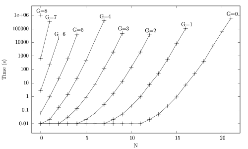
Figure 2. Time needed to compute all stable graphs of type $(G,N)$.

$G$	$N$	Time (s)	# stable graphs	Duplicates (%)
0	18	392	847,511	54.9
1	14	539	1,832,119	41.3
2	10	147	1,282,008	30.9
3	7	117	1,280,752	29.9
4	5	459	2,543,211	40.1
5	3	606	2,575,193	54.7
6	1	226	962,172	70.6
7	0	681	1,281,678	85.6

Table 1. For small $G$, the maximum $N$ such that all stable graphs of type $(G,N)$ can be computed in less than $15$ minutes. In the last column we show the ratio of duplicated graphs among the total number of those created by our generation algorithm.

In Table 1 we list, for each genus $G$, the maximum number of marked points $N$ for which we can compute all the stable graphs of type $(G,N)$ under 15 minutes.

In Figure 2 we show all the couples $(G,N)$ that we computed against the time needed; the lines connect the results referring to the same genus. From this plot it seems that, for fixed $G$, the required time increases exponentially with $N$. However, we believe that in the long run the behaviour will be worse than exponential. This is suggested also by the fact that the ratio of non-isomorphic stable graphs over those created by our generation algorithm tends to zero as $G$ and $N$ grow (see Figure 3).

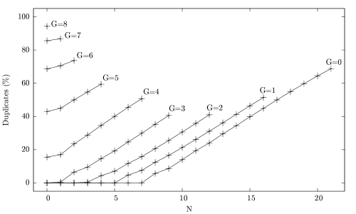
Figure 3. Ratio of duplicated graphs among the total number of those created by our generation algorithm.

More benchmarks and up-to-date computed results are available at boundary’s webpage, http://people.sissa.it/~maggiolo/boundary/.

References

- [BMS] S. Busonero, M. Melo, and L. Stoppino, On the complexity group of stable curves, Adv. in Geometry 11 (2011), no. 2, 241–272, [arXiv:0808.1529].
- [DM] P. Deligne and D. Mumford, The irreducibility of the space of curves of given genus, Inst. Hautes Études Sci. Publ. Math. 36 (1969), 75–109.
- [F] C. Faber, Maple program for computing Hodge integrals, available at http://math.stanford.edu/~vakil/programs/.
- [GK] E. Getzler and M. Kapranov, Modular Operads, Compositio Math. 110 (1998), no. 1, 65–126 [arXiv:dg-ga/9408003].
- [K] F. Knudsen, Projectivity of the moduli space of stable curves II. The stacks , Math. Scand. 52 (1983), 161–199.
- [M] B. D. McKay, nauty, available at http://cs.anu.edu.au/people/bdm/nauty/.
- [vOV1] M. A. van Opstall and R. Veliche, Maximally symmetric stable curves, Michigan Math. J. 55 (2007), no. 3, 513–534 [arXiv:math/0603061].
- [vOV2] M. A. van Opstall and R. Veliche, Maximally symmetric stable curves II, arXiv:math/0608799.
- [Y1] S. Yang, Intersection numbers on , Journal of Software for Algebra and Geometry, 2 (2010), 1–5.
- [Y2] S. Yang, Maple program for computing integrals on , available by request from author stpyang@math.kth.se.
- [Y3] S. Yang, Calculating intersection numbers on moduli spaces of pointed curves, arXiv:0808.1974.