Physics of high energy atmospheric muons

Abstract

In the first part of the talk the interesting new results of MINOS, OPERA and CMS collaborations (connected with the observational evidence of the rise in the muon charge ratio at muon energies around 1 TeV) are briefly discussed from theoretical point of view. A short review of charge asymmetric effects in muon energy losses is given. In the second part of the talk, the modern theoretical approaches to the problem of heavy quark production in high energy nucleon-nucleus interactions are briefly considered (color dipole formalism, saturation models). The recent new theoretical developments in the ancient problem of intrinsic charm are also discussed.

I THE CHARGE RATIO OF ATMOSPHERIC MUONS

I.1 Pika model

A simple formula for the muon atmospheric charge ratio is obtained from the approximate expression for the differential atmospheric muon spectrum ZK1960 ; Gaisser1990 :

$$\frac{d\phi_{\mu}}{dE_{\mu}}\cong\frac{d\phi_{N}}{dE_{\mu}}\sum_{i}\frac{a_{i}Z_{Ni}}{1+b_{i}E_{\mu}\cos\theta^{*}/\epsilon_{i}},$$ (1)

where $d\phi_{N}/dE_{\mu}\equiv d\phi_{N}/dE$ (at $E=E_{\mu}$) is the primary spectrum of nucleons ($E_{\mu}$ is the muon energy in atmosphere), index $i$ numerates muon parents ($\pi$, $K$ etc), the constants $a_{i}$, $b_{i}$ are purely kinematical (they depend on the characteristics of parent’s decay into muons), $\epsilon_{i}$ are the critical energies, which are defined as parent’s energies in atmosphere, at which their interaction lengths are equal to decay lengths (for a vertical propagation), $\theta^{*}$ is the zenith angle of the muon trajectory (for simplicity, we assume that atmosphere is flat). At last, $Z_{ij}$ is the spectrum weighted moment defined by the expression

$$Z_{ij}=\int\limits_{0}^{1}\frac{1}{\sigma_{ij}}\frac{d\sigma_{ij}}{dx_{lab}}x_{lab}^{\gamma-1}dx_{lab},$$ (2)

where $\sigma_{ij}$ is the inclusive cross-section for the production of a particle $j$ from the collision of a particle $i$ with a nucleus in the atmosphere and $x_{lab}=E_{j}/E_{i}$ is the energy fraction carried by the secondary particle, $\gamma$ is a spectral index of the primary nucleon spectrum, $\gamma=1.7$.

If we are interested in the interval of muon energies $(1-10^{4})\;$GeV, one can take into account only pions and kaons as muon’s parents. In this case, the muon spectrum can be expressed as

$$\frac{d\phi_{\mu^{\pm}}}{dE_{\mu}}\cong\frac{a_{\pi}f_{\pi^{\pm}}}{1+b_{\pi}E_{\mu}\cos\theta^{*}/\epsilon_{\pi}}+\frac{R_{K\pi}a_{K}f_{K^{\pm}}}{1+b_{K}E_{\mu}\cos\theta^{*}/\epsilon_{K}},$$ (3)

where $R_{K\pi}=Z_{NK}/Z_{N\pi}$ and $f_{\pi^{+}}=1-f_{\pi^{-}}=Z_{N\pi^{+}}/Z_{N\pi}$, $f_{K^{+}}=1-f_{K^{-}}=Z_{NK^{+}}/Z_{NK}$ are fractions of all pion and kaon decays that yield positive muons. This simple formula used for an analysis of atmospheric muon charge ratio data is a basic of the so-called “pika model” Schreiner:2009pf . More exactly, this model uses the following main assumptions: 1) particle ratios, $\pi^{+}/\pi^{-}=f_{\pi^{+}}$ and $K^{+}/K^{-}=f_{K^{+}}$, are energy independent; $K/\pi$ ratio is given by the $R_{K\pi}\cdot a_{K}/a_{\pi}=0.149\cdot 0.246/0.674=0.054$ Gaisser1990 , 2) all the spectrum weighted moments, $Z_{ij}$, are energy independent, 3) the muon charge ratio does not depend on the $E_{\mu}$ and the $\cos\theta^{*}$ separately, but on the product $E_{\mu}\cos\theta^{*}$, where $E_{\mu}$ is the energy of vertical muons on the Earth surface, 4) contributions from charmed mesons are ignored.

I.2 Particle ratios

It is well known from studies of $K$-production in $NN$ and $NA$-collisions, in the energy region near the threshold, that $K^{+}/K^{-}$ ratio is rather large. The explanation is simple: $K^{+}$-meson contains $\bar{s}$-quark whereas, for a final baryon, $s$-quark is needed. The transfer of $s$-quark from $K^{-}$-meson to a final baryon is realized most effectively through the reaction $K^{-}N\to\pi\Lambda$. So, as a result, the escape of $K^{-}$-mesons is hampered. Measurements of particle ratios at high energies, far from the threshold of $K$ production, shows (see, e.g., the data of the BRAHMS Collaboration Bearden:2004ya for $pp$-collisions at $\sqrt{s}=200\;$GeV) that, at large rapidities (close to the fragmentation region), the $K^{+}/K^{-}$-ratios are systematically larger than $\pi^{+}/\pi^{-}$-ratios. In general, such asymmetries in the production of particles and antiparticles are indications of the leading particle effects in hadronic collisions and are rather intensively studied now experimentally as well as theoretically. In particular, large values of $K^{+}/K^{-}$-ratios measured by Bearden:2004ya are well explained by the DPM JET model Bopp:2005cr .

I.3 Muon energy losses: $z$-odd effects

I.3.1 Ionization energy losses

As is known, the standard expression for energy loss contains, except of the main term, proportional to $z^{2}$, the tiny term which is proportional to $\frac{\pi\alpha}{2}z^{3}$ ($\alpha$ is the fine structure constant) Jackson:1972zz . This term is due to the next-to-leading order correction to the relativistic Rutherford formula. The $z^{3}$-correction to $dE/dx$ is taken into account in an analysis of data in the MINOS experiment Schreiner:2009pf as well as in the CMS Khachatryan:2010mw , in spite of its smallness. For $\mu^{+}$, the energy loss in matter is about $\sim 0.15\%$ higher than for $\mu^{-}$, for CMS experiment, and it affects the muon charge ratio by less than $\sim 0.3\%$ over the entire energy range Khachatryan:2010mw .

I.3.2 Radiative energy losses

The muon bremsstrahlung cross section is given by the formula

$$\omega\frac{d\sigma}{d\omega}=\omega\left.\frac{d\sigma}{d\omega}\right|_{Born}+\Delta_{c}+\Delta_{DBM}+\Delta_{nonleading}.$$ (4)

Here, $\omega$ is the photon energy, the first term in r.h.s. is the cross section calculated in the Born approximation (including, in this approximation, the nuclear formfactor correction), $\Delta_{c}$ is the “non-Coulomb” correction Andreev:1997pf (it is important only for muons and is the non-Born part of the correction which arises due to the non-Coulombic character of the electromagnetic field of the nucleus having the extended size), $\Delta_{DBM}$ is the well-known Coulomb correction of Davies, Bethe and Maximon Davies:1954zz . At last, $\Delta_{nonleading}$ takes into account the main correction to ultrarelativistic approximation which had been used before for a calculation of all components of the bremsstrahlung cross section. It appears Lee:2004ina that this correction is proportional to $-\frac{m_{\mu}}{E_{\mu}}Z\alpha$, the minus sign corresponds to the $\mu^{-}$, i.e., the $\mu^{+}$ has again a slightly larger energy loss. So, the difference between the $\mu^{+}$ and $\mu^{-}$ energy losses due to bremsstrahlung is inversely proportional to the muon $\gamma$-factor,

$$\left[\frac{dE}{dx}\right]^{\mu^{+}}-\left[\frac{dE}{dx}\right]^{\mu^{-}}\sim\frac{Z\alpha}{\gamma}\langle\frac{dE}{dx}\rangle,$$ (5)

and is very small for the case of the rock ($Z=11$). This difference is negligible Schreiner:2009pf in the region around $E_{\mu}\sim(0.1-1)\;$TeV, where radiative energy losses become comparable with ionization energy losses.

Figure 1: $R_{\mu}$ values measured by OPERA, MINOS and other experiments (taken from Agafonova:2010fg ).

One should note that, of course, there are other sources of the charge asymmetry in muon energy losses. For example, in the process of $e^{+}e^{-}$-pair production by muon on atomic electrons such an asymmetry arises due to interferences of different diagrams contributing to the process Kelner:1998mh . One should mention, in this connection, also the work Kelner:1999yf in which diffractive corrections to muon bremsstrahlung had been considered.

I.4 Conclusions

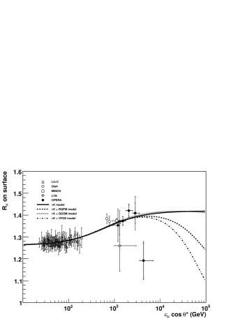
1. The recent experimental results of three groups, MINOS Schreiner:2009pf , OPERA Agafonova:2010fg and CMS Khachatryan:2010mw (together with the old result of Utah detector Ashley:1975uj ) show that the atmospheric muon charge ratio at energies around 1 TeV and higher is sizeably larger ($R_{\mu}\sim 1.36-1.4$) than at energies around $\sim 10^{2}\;$GeV (see Fig. 1).

2. The data fittings give the similar results for all three groups: $r_{\pi}=f_{\pi^{+}}/(1-f_{\pi^{+}})=1.241\pm 0.035$, $r_{K}=f_{K^{+}}/(1-f_{K^{+}})=2.26\pm 0.29$ (MINOS N+F Schreiner:2009pf ); $r_{\pi}=1.229\pm 0.001$, $r_{K}=2.12\pm 0.03$ (OPERA Agafonova:2010fg ); $f_{\pi^{+}}=0.553\pm 0.005$, $f_{K^{+}}=0.66\pm 0.06$ (CMS Khachatryan:2010mw ).

3. The increase of the ratio $R_{\mu}$ is due to the fact that i) according to the pika model, at energies $\gtrsim 1\;$TeV, the contribution of kaons in $R_{\mu}$ becomes dominant, and ii) for kaons, the ratio $K^{+}/K^{-}$ is larger than the corresponding ratio for pions.

4. The fits of the pika formula to the old results of calculations Lipari1993 and simulations Honda:1995hz ; Fiorentini:2001wa lead to the following numbers Schreiner:2009pf : $r_{K}=2.87$, $r_{\pi}=1.25$ (for the calculation by Lipari Lipari1993 ); $r_{K}=2.39$, $r_{\pi}=1.26$ (for the simulations with CORT code Fiorentini:2001wa ); $r_{K}=1.63$, $r_{\pi}=1.28$ (for the simulations by Honda Honda:1995hz ).

5. It would be quite interesting to check whether the recent experimental results Bearden:2004ya and theoretical predictions Bopp:2005cr are consistent with the new $R_{\mu}$-data.

II CHARM PRODUCTION IN $pA$-COLLISIONS AND PROMPT MUONS

II.1 Introduction

One can see from Fig. 1 that the value of $R_{\mu}$ at $E_{\mu}\gtrsim 10\;$TeV strongly depends on the charm production model. It is well known that it is not so difficult to calculate muon atmospheric fluxes, but only if you know well the fluxes of muon parents (charmed mesons, in a given case). So, the physics of hadronic charm production is intimately connected with physics of atmospheric high energy muons.

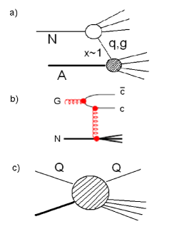
The schematic diagram of the process is shown in Fig 2a. We consider in this talk only two examples of such calculations.

1. If one uses perturbative QCD approach, the typical diagram for the lower blob of diagram a) is shown in Fig. 2b (gluon fusion).

2. If it is assumed that there are non-perturbative “intrinsic” heavy quark components in the proton wave function Brodsky:1980pb , the diagram in the lower blob of a) describes the inclusive scattering of the heavy quark of the proton projectile on the target (Fig. 2c).

The common points in these cases are following: the fragmentation region of the proton projectile is of interest; the target is a nucleus; the proton energy is very high ( $>100TeV$). We will show in this talk that both cases can be studied using the modern approach to high energy scattering in QCD based on the idea of the Color Glass Condensate (CGC) (for a review, see Iancu:2003xm ).

Figure 2: The schematic diagrams of the $pA$-collision.

II.2 CGC framework

II.2.1 Dipole cross section

In the CGC approach, the proton and the target nucleus are effectively described as static random sources of color charge on the light cone. The leading contribution to particle production in $pA$-collisions is obtained by calculating the classical color field created by these sources and then averaging over a random distribution McLerran:1993ni .

The field is a solution of the classical Yang-Mills equation:

$$\left[D_{\mu},F^{\mu\nu}\right]=J^{\nu},$$ (6)

where $J^{\nu}$ is the classical current which is determined by the sources $\rho_{p}$ and $\rho_{A}$:

$$J^{\nu}_{a}=g\delta^{\nu+}\delta(x^{-})\rho_{p,a}(\vec{x}_{\perp})+g\delta^{\nu-}\delta(x^{+})\rho_{A,a}(\vec{x}_{\perp}).$$ (7)

Here, $x^{\pm}=\frac{x^{0}\pm x^{3}}{\sqrt{2}}$, $\vec{x}_{\perp}$ is the transverse component of $\vec{x}$, $x^{+}$ is the “LC time”. $\rho_{p},\rho_{A}$ are static, i.e., independent of the LC time. $\delta(x^{-})$ function assumes an infinitely thin sheet of color charge.

It is shown in many works that in CGC approach (see, e.g., Gelis:2002nn ) the amplitude for a scattering of a quark from the target, $qA\to qX$, is expressed through the “gauge rotation” matrix $U(\vec{x}_{\perp})$:

$${\cal M}_{qA\to qX}=\bar{u}(q)\times\;\;\;\;\;\;\;\;\;\;\;\;\;\;\;\;\;\;\;\;\;\;\;\;\;\;\;\;\;\;\;\;\;\;\;\;\;\;\;\;\;\;\;\;\;\;$$

$$\times\left[\gamma^{-}\int d^{2}x_{\perp}e^{i(q_{\perp}-p_{\perp})x_{\perp}}\left(U(\vec{x}_{\perp})-1\right)\right]u(p).\;\;\;$$ (8)

This matrix is given by the expression:

$$U(\vec{x}_{\perp})=T\exp\left[-ig^{2}\int\limits_{-\infty}^{\infty}dx^{+}\frac{1}{\Delta_{\perp}^{2}}\rho_{A,a}(x^{+},x_{\perp})t^{a}\right],$$ (9)

$t^{a}$ is a color matrix, generator of the fundamental representation of $SU(N_{c})$. Here, $\rho_{A,a}(\vec{x})$ is the density of color sources in the nucleus in the covariant gauge $\partial_{\mu}A^{\mu}=0$. For concrete calculations the LC-gauge, in which $A^{+}=0$, is used, because in this gauge the color fields depend only on the matrix $U$ (i.e., they are “pure gauge” fields). But $U$ depends on the $\rho_{A,a}(\vec{x})$, the density of sources in the covariant gauge.

It is very important that the same matrix $U(\vec{x}_{\perp})$ enters the expression for the dipole-hadron cross section, $\sigma_{\rm dip}(\vec{r}_{\perp})$, which is the total cross section of interaction with nucleus, for a dipole of transverse size $\vec{r}_{\perp}=\vec{x}_{\perp}-\vec{y}_{\perp}$ (with the quark located at $\vec{x}_{\perp}$ and the antiquark at $\vec{y}_{\perp}$ ) and is written as an integral over all the impact parameters $\vec{X}_{\perp}=(\vec{x}_{\perp}+\vec{y}_{\perp})/2$,

$$\sigma_{\rm dip}(\vec{r}_{\perp})\equiv\frac{2}{N_{c}}\int d^{2}\vec{X}_{\perp}{\rm Tr_{c}}\langle 1-\;\;\;\;\;\;\;\;\;\;\;\;\;\;\;\;\;\;\;\;\;$$

$$-U\left(\vec{X}_{\perp}+\frac{\vec{r}_{\perp}}{2}\right)U^{+}\left(\vec{X}_{\perp}-\frac{\vec{r}_{\perp}}{2}\right)\rangle_{\rho}.$$ (10)

We will see, in the next Section, that charm production cross sections contain just the $\sigma_{\rm dip}(\vec{r}_{\perp})$, which is expressed, as is seen from Eq. (10), through the 2-point function, or “2-point correlator”, $\langle U(x_{\perp})U^{+}(y_{\perp})\rangle$. In the Eq. (10), ${\rm Tr}_{c}$ is the color trace ($U$ is the matrix in the color space), and ensemble average is performed over the sources. In the McLerran-Venugopalan (M-V) McLerran:1993ni model a Gaussian distribution of color sources is used,

$$W[\rho]=\exp\left[-\int dx^{+}d^{2}x_{\perp}\frac{\rho_{a}(x^{+},\vec{x}_{\perp})\rho^{a}(x^{+},\vec{x}_{\perp})}{2\mu_{A}^{2}(x^{+})}\right],$$ (11)

$$\langle{\cal O}\rangle\equiv\int[d\rho]W[\rho]{\cal O}[\rho].$$ (12)

The color source is “frozen” through the collision due to time dilation but changes from the collision to the subsequent one. Evidently, $\mu_{A}^{2}(x^{+})$ is a density of color sources per unit volume and

$$\mu_{A}^{2}=\int dx^{+}\mu_{A}^{2}(x^{+})$$ (13)

is the average density of the sources per unit transverse area,

$$\langle\rho_{a}(\vec{x}_{\perp})\rho_{b}(\vec{y}_{\perp})\rangle=\delta_{ab}\delta(\vec{x}_{\perp}-\vec{y}_{\perp})\mu_{A}^{2},\;\;\;\mu_{A}^{2}\sim A^{1/3}.$$ (14)

The straightforward calculation gives for $\sigma_{\rm dip}(\vec{r}_{\perp})$ the result (if the target is homogeneous in the transverse plane):

$$\sigma_{\rm dip}(\vec{r}_{\perp})=2\pi R^{2}\left[1-\exp\left(-Q_{s}^{2}f(r_{\perp})\right)\right],$$ (15)

where $f(r_{\perp})$ is the known function and $Q_{s}^{2}$ is given by

$$Q_{s}^{2}=\frac{g^{4}}{2}(t^{a}t_{a})\mu_{A}^{2}=\frac{g^{4}}{2}\frac{N_{c}^{2}-1}{2N_{c}}\mu_{A}^{2}\sim\alpha_{s}^{2}A^{1/3}.$$ (16)

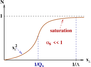
By definition, $Q_{s}^{2}$ is the saturation scale (in the M-V model). The schematic form of $\sigma_{\rm dip}(\vec{r}_{\perp})$ is shown in Fig. 3.

Figure 3: The forward dipole amplitude, $\sigma_{\rm dip}/2\pi R^{2}$, as a function of the transverse separation between $q$ and $\bar{q}$ (taken from JalilianMarian:2005jf ).

Taking into account the quantum corrections Iancu:2003xm , one can show that the dipole cross section can be parameterized in the following form Kharzeev:2004yx :

$$\sigma_{\rm dip}(r_{\perp},x)\approx 2\pi R_{A}^{2}\left(1-\exp(-\frac{(Q_{s}^{2}(x)r_{\perp}^{2})^{\gamma}}{4})\right),$$ (17)

$$\frac{Q_{s}^{2}(x)}{1\;{\rm GeV}^{2}}=\frac{N_{c}^{2}-1}{2N_{c}}\left(\frac{x_{0}}{x}\right)^{\lambda}A^{1/3},$$ (18)

$$x_{0}\approx 3\times 10^{-4},\;\lambda\approx 0.3,\;\gamma\approx 0.628.$$ (19)

It follows from this equation that the saturation scale $Q_{s}^{2}$ becomes dependent on energy, because the dipole cross section depend now on Bjorken $x$. In DIS, the value of $x$ is connected with the photon virtuality,

$$x=\frac{Q^{2}}{2Mq_{0}}.$$ (20)

In a case of the inclusive hadronic scattering and, in particular, in the case of heavy quark production in hadronic collisions, $x$ is the momentum fraction of the target parton participating in the reaction ($x=x_{A}$).

II.2.2 Kinematics of reactions

1. In the case of intrinsic charm production (Fig. 2c), there is the simple connection between $x_{A}$ and the momentum fraction of the projectile ($x_{p}$):

$$x_{A}=\frac{x_{p}q_{t}^{2}}{x_{F}^{2}s};\;\;x_{A}\equiv x_{p}e^{-2y_{h}},$$ (21)

where $x_{F}$ is the Feynman $x$ of the produced particle; $y_{h}$ is its rapidity, $q_{t}$ is its transverse momentum. In the forward region one has

$$x_{F}\to 1;\;\;\;1\leq x_{p}\leq x_{F},\;\;{\rm and}\;\;\;\;\langle x_{A}\rangle\to\frac{q_{t}^{2}}{s}\to 0.$$ (22)

2. In the case of extrinsic charm production (Fig. 2b) we have two colliding gluons, with momentum fractions $x_{g}$ and $x_{A}$. Assume, for simplicity, that the heavy quark pair is produced with Feynman $x_{F}$ corresponding to a fixed $M_{Q\bar{Q}}$. One has

$$x_{A}=\left(\sqrt{x_{F}^{2}+\frac{4M_{Q\bar{Q}}^{2}}{s}}-x_{F}\right)\frac{1}{2},\;\;\;\;\;x_{g}=x_{F}+x_{A},$$ (23)

and, again, in the forward region, $x_{A}\sim M_{Q\bar{Q}}^{2}/s\to 0$.

II.2.3 Target description in a small $x$ region

1. Coherent lengths of small x partons in the target are very large, $\ell\sim 1/(M_{N}x)$, much larger than the nuclear size. Therefore, at very small Bjorken $x$ inclusive particles are produced in hadron-nucleus collisions coherently by the nuclear color field.

2. The gluon distribution which is the number of gluons per unit rapidity in the hadron wave function,

$$xG(x,Q^{2})=dN_{\rm gluons}/dy,$$ (24)

grows with the decrease of $x$; as a result, the saturation scale $Q_{s}^{2}$ also grows:

$$Q_{s}^{2}\sim A^{1/3}/x^{\lambda}.$$ (25)

Physically, $Q_{s}^{2}$ is the average color charge squared of the gluons per unit transverse area per unit rapidity.

3. If the density of color charge grows, the classical description of the color field becomes possible as a first approximation McLerran:1993ni . The nonlinear effects in the classical Yang-Mills equations and quantum evolution corrections lead to a saturation of gluon distributions.

One should note that the experimental as well as theoretical study of heavy quark production at forward rapidities is very important just for the “saturation physics” because the saturation scale $Q_{s}$ increases with energy, $Q_{s}\sim A^{1/6}s^{\lambda/4}$, and, at large $A$ and $s$, can be larger than $M_{q}$. The typical transverse momenta of partons in the hadron are of the same order as $Q_{s}$ , so, it is natural to expect that in such cases the probability of $QQ$-pair production will be greatly enhanced.

II.3 Extrinsic and intrinsic charm production

Figure 4: The comparison of the predictions of the dipole model Enberg:2008te with the corresponding predictions of the pQCD model Pasquali:1998ji , for different proton energies (taken from Enberg:2008te ).

Figure 5: The prompt muon flux predicted by dipole model Enberg:2008te ($\nu_{\mu}+\tilde{\nu}_{\mu}$, $\nu_{e}+\tilde{\nu}_{e}$ and $\mu^{+}+\mu^{-}$ - fluxes are approximately equal). Conventional fluxes are represented by dashed lines Gondolo:1995fq . The figure is taken from Enberg:2008te .

II.3.1 Extrinsic charm in the color dipole approach

In the model of Nikolaev:1995ty ; Kopeliovich:2002yv the differential cross section is

$$\frac{d\sigma}{dy}(pA\to Q\bar{Q}X)\cong x_{g}G(x_{g},\mu^{2})\sigma^{GA\to Q\bar{Q}X}(x_{A},\mu^{2}),$$ (26)

$$\sigma^{GA\to Q\bar{Q}X}(x_{A},\mu^{2})\cong\int dzd^{2}r_{\perp}|\Psi_{G}|^{2}\sigma_{\rm dip}(x_{A},r_{\perp}).$$ (27)

Here, $|\Psi_{G}(z,\vec{r}_{\perp})|^{2}$ is the probability of finding $QQ$-pair with a separation $r_{\perp}$ and a fractional momentum $z$ in the gluon, $\mu\sim m_{Q}$ is the factorization scale. The cross section is written in a factorized form and contains $\sigma_{\rm dip}(x_{A},r_{\perp})$ which depends only on two-point correlator $\langle U(x_{\perp})U^{+}(y_{\perp})\rangle$. It is a consequence of the special choice of perturbative diagrams. In general, if the nuclear color field is strong, one must take into account all orders in $\rho_{A}$ (if $g^{2}\rho_{A}\sim 1$) and, in particular, include diagrams with exchange of two gluons Blaizot:2004wv . After this there will be no simple factorization: the cross section will depend on 2-point, 3-point and 4-point correlators.

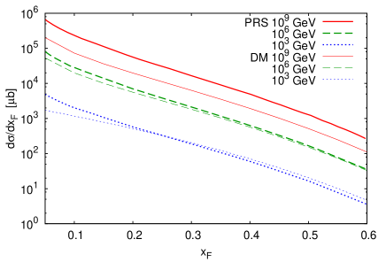
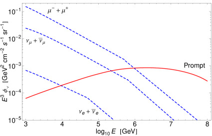
On Fig. 4, the predictions of this model Enberg:2008te are shown, for several incident proton energies, with a comparison with the corresponding results of pQCD model Pasquali:1998ji . One can clearly see the suppression of charm production at very high energies due to gluon saturation effects. On the Fig. 5, the prediction of the same model Enberg:2008te for the prompt lepton fluxes are shown (in comparison with the conventional fluxes Gondolo:1995fq ).

II.3.2 Intrinsic charm production.

In the CGC approach, the diagram of the inclusive heavy quark scattering (Fig. 2c) is the basic one. The amplitude of this scattering is given by Eq. (8).

After squaring this amplitude, one obtains, again, the formula containing 2-point correlator, which can be expressed through the dipole-hadron cross section $\sigma_{\rm dip}$. The formula for the inclusive production of the charmed meson is Dumitru:2005gt ; Goncalves:2008sw :

$$\frac{d\sigma(pA\to DX)}{dyd^{2}p_{\perp}}=\frac{1}{(2\pi)^{2}}\int\limits_{x_{F}}^{1}dx_{p}\frac{x_{p}}{x_{F}}f_{c/p}(x_{p},Q^{2})\times$$

$$\times\int d^{2}r_{\perp}e^{i\vec{q}_{\perp}\vec{r}_{\perp}}\frac{\sigma_{\rm dip}(r_{\perp},x_{A})}{2}D_{D/c}\big{(}\frac{x_{F}}{x_{p}},Q^{2}\big{)}.\;\;\;$$ (28)

The existence of an “intrinsic charm” (IC) component of the nucleon is not forbidden. Many nonperturbative models predict such a component at an energy scale comparable to mass of charm quark $m_{c}$. In Bugaev:2009jw , the predictions of the specific light-cone model developed in Brodsky:1980pb (“BHPS model”) are used for the calculation of charm production (authors of Brodsky:1980pb calculated the PDF of charm quarks from the 5-quark component $uudcc$ in the proton). As a second example, authors of Bugaev:2009jw considered the phenomenological model Pumplin:2007wg , in which the shape of the charm PDF is sea-like, i.e., similar to that of the light flavor sea quarks (except for normalization). In the concrete calculation, the scale dependence of PDFs must be taken into account. For this aim, authors of Bugaev:2009jw used the PDFs from the work Pumplin:2007wg , based on the calculations of CTEQ group. For BHPS model, it was assumed, in Bugaev:2009jw , that the charm content of the proton is on the maximal level, $\langle x\rangle_{c+\bar{c}}=0.02$. The same is for the sea-like IC model: $\langle x\rangle_{c+\bar{c}}=0.024$.

Figure 6: The comparison of $x_{F}$-spectra for BHPS (solid) and sea-like (dashed) models, for two energies, $\sqrt{s}=10^{2}$ and $10^{4}$ GeV ($A=14$, from Bugaev:2009jw ).

Figure 7: The comparison of the results of Bugaev:2009jw (thick) with the results of Goncalves:2006ch (thin), for $E_{p}=10^{9}$ GeV (upper curves) and $3.4\times 10^{4}$ GeV (lower curves); $A=14$.

On the following two figures some results of the recent work Bugaev:2009jw are presented. Fig. 6 gives the comparison of $x_{F}$-spectra for two different models of the intrinsic charm. On Fig. 7 the comparison of the predictions for inclusive cross sections for intrinsic Bugaev:2009jw (the total contribution of all mesons) and extrinsic charm Goncalves:2006ch is shown. Authors of Goncalves:2006ch used the dipole model approach and their results are similar with the results of Enberg:2008te .

Figure 8: The total cross section of charm production in $pp$ collisions at $p>400GeV/c$ Merino:2007rg . At high energies, squares correspond to PHENIX data and triangles to STAR data. The data of cosmic rays Rakobolslaya are shown by diamonds. The figure is taken from Merino:2007rg .

It follows from figure 7 that in the tail region, $x_{F}>0.7$, the curves of Bugaev:2009jw are even steeper than those of Goncalves:2006ch , in spite of their “intrinsic” origin. One must bear in mind, however, that in Bugaev:2009jw the inclusive spectra of charmed hadrons rather than $c\bar{c}$ pairs are calculated. Naturally, a taking into account of the fragmentation of $c$ quarks into hadrons leads to additional steepening of $x_{F}$-spectra.

II.3.3 Experimental data of RHIC

One can see from the Fig. 8 that the results of different pQCD approaches (presented on the Figure by curves) underestimate, in general, the cross section of charm production at high energies. Authors of Merino:2007rg argue, that it may be connected, in particular, with large non-perturbative contributions in high density states (e.g., with CGC effects).

II.4 Conclusions

We tried to show in this review that the modern approach to studies of proton-nucleus nucleus interactions based on the CGC theory can be effectively used in calculations of heavy quark production in $pA$ collisions. The most important application of this approach is an use of it in calculations of open charm production in collisions of cosmic rays in atmosphere (needed for subsequent calculations of prompt muon and neutrino fluxes at energies around 100 TeV and higher). The reason is simple: in collisions of cosmic rays in atmosphere, the fragmentation region of the projectile (or forward rapidity region) is most important for calculations of all spectra of secondary particles, and just in this region the effects of gluon saturation studied in CGC theory are most efficient.

References

- (1) G. T. Zatsepin and V. A. Kuz’min, Zh. Eksp. Teor. Fiz., 39, 1677 (1960); Sov. Phys. JETP, 12, 1171 (1961).
- (2) T. Gaisser, “Cosmic Rays and Particle Physics”, Cambridge University Press, 1990.
- (3) P. A. Schreiner, J. Reichenbacher and M. C. Goodman, Astropart. Phys. 32, 61 (2009) [arXiv:0906.3726 [hep-ph]].
- (4) I. G. Bearden et al. [BRAHMS Collaboration], Phys. Lett. B 607, 42 (2005) [arXiv:nucl-ex/0409002].
- (5) F. W. Bopp, J. Ranft, R. Engel et al., Phys. Rev. C77, 014904 (2008) [hep-ph/0505035].
- (6) J. D. Jackson and R. L. McCarthy, Phys. Rev. B 6, 4131 (1972).
- (7) V. Khachatryan et al. [CMS Collaboration], Phys. Lett. B 692, 83 (2010) [arXiv:1005.5332 [hep-ex]].
- (8) Yu. M. Andreev and E. V. Bugaev, Phys. Rev. D 55, 1233 (1997).
- (9) H. Davies, H. A. Bethe, L. C. Maximon, Phys. Rev. 93, 788-795 (1954).
- (10) R. N. Lee, A. I. Milstein, V. M. Strakhovenko and O. Y. Schwarz, J. Exp. Theor. Phys. 100, 1 (2005) [Zh. Eksp. Teor. Fiz. 100, 5 (2005)] [arXiv:hep-ph/0404224].
- (11) S. R. Kelner, Phys. Atom. Nucl. 61, 448 (1998) [Yad. Fiz. 61, 511 (1998)].
- (12) S. R. Kelner and A. M. Fedotov, Phys. Atom. Nucl. 62, 272 (1999) [Yad. Fiz. 62, 307 (1999)].
- (13) N. Agafonova et al. [OPERA Collaboration], Eur. Phys. J. C 67, 25 (2010) [arXiv:1003.1907 [hep-ex]].
- (14) G. K. Ashley, J. W. Keuffel and M. O. Larson, Phys. Rev. D 12, 20 (1975).
- (15) P. Lipari, Astropart. Phys. 1, 195 (1993).
- (16) G. Fiorentini, V. A. Naumov and F. L. Villante, Phys. Lett. B 510, 173 (2001) [arXiv:hep-ph/0103322].
- (17) M. Honda, T. Kajita, K. Kasahara and S. Midorikawa, Phys. Rev. D 52, 4985 (1995) [arXiv:hep-ph/9503439].
- (18) S. J. Brodsky, P. Hoyer, C. Peterson and N. Sakai, Phys. Lett. B 93, 451 (1980).
- (19) E. Iancu and R. Venugopalan, arXiv:hep-ph/0303204.
- (20) L. D. McLerran and R. Venugopalan, Phys. Rev. D 49, 2233 (1994) [arXiv:hep-ph/9309289].
- (21) F. Gelis and J. Jalilian-Marian, Phys. Rev. D 67, 074019 (2003) [arXiv:hep-ph/0211363].
- (22) J. Jalilian-Marian and Y. V. Kovchegov, Prog. Part. Nucl. Phys. 56, 104 (2006) [arXiv:hep-ph/0505052].
- (23) D. Kharzeev, Y. V. Kovchegov and K. Tuchin, Phys. Lett. B 599, 23 (2004) [arXiv:hep-ph/0405045].
- (24) B. Z. Kopeliovich and A. V. Tarasov, Nucl. Phys. A 710, 180 (2002) [arXiv:hep-ph/0205151].
- (25) N. N. Nikolaev, G. Piller and B. G. Zakharov, Z. Phys. A 354, 99 (1996) [arXiv:hep-ph/9511384].
- (26) J. P. Blaizot, F. Gelis and R. Venugopalan, Nucl. Phys. A 743, 57 (2004) [arXiv:hep-ph/0402257].
- (27) R. Enberg, M. H. Reno and I. Sarcevic, Phys. Rev. D 78, 043005 (2008) [arXiv:0806.0418 [hep-ph]].
- (28) L. Pasquali, M. H. Reno, I. Sarcevic, Phys. Rev. D59, 034020 (1999) [hep-ph/9806428].
- (29) P. Gondolo, G. Ingelman, M. Thunman, Astropart. Phys. 5, 309-332 (1996) [hep-ph/9505417].
- (30) A. Dumitru, A. Hayashigaki and J. Jalilian-Marian, Nucl. Phys. A 765, 464 (2006) [arXiv:hep-ph/0506308].
- (31) V. P. Goncalves and F. S. Navarra, Nucl. Phys. A 842, 59 (2010) [arXiv:0805.0810 [hep-ph]].
- (32) E. V. Bugaev and P. A. Klimai, J. Phys. G 37, 055004 (2010) [arXiv:0905.2309 [hep-ph]].
- (33) J. Pumplin, H. L. Lai and W. K. Tung, Phys. Rev. D 75, 054029 (2007) [arXiv:hep-ph/0701220].
- (34) V. P. Goncalves and M. V. T. Machado, JHEP 0704, 028 (2007) [arXiv:hep-ph/0607125].
- (35) C. Merino, C. Pajares and Yu. M. Shabelski, arXiv:0707.0946 [hep-ph].
- (36) I. V. Rakobolslaya, T. M. Roganova, L. G. Sveshnikova, Nucl. Phys. B (Proc. Suppl.) 122, 353 (2003).