Some properties of skew-symmetric distributions

Abstract

The family of skew-symmetric distributions is a wide set of probability density functions obtained by combining in a suitable form a few components which are selectable quite freely provided some simple requirements are satisfied. Intense recent work has produced several results for specific sub-families of this construction, but much less is known in general terms. The present paper explores some questions within this framework, and provides conditions on the above-mentioned components to ensure that the final distribution enjoys specific properties.

Primary Subjects: 60E05 62H10

Secondary Subjects: 62E15, 60E15

Key-words: central symmetry, log-concavity, peakedness, quasi-concavity, skew-symmetric distributions, stochastic ordering, strong unimodality, unimodality.

1 Introduction and motivation

1.1 Distributions generated by perturbation of symmetry

In recent years, there has been quite an intense activity connected to a broad class of continuous probability distributions which are generated starting from a symmetric density functions and applying a suitable form of perturbation of the symmetry. The key representative of this formulation is the so-called skew-normal distribution, whose density function in the scalar case is given by

$$f(x;\alpha)=2\,\phi(x)\,\Phi(\alpha\,x),\qquad\qquad(x\in\mathbb{R}),$$ (1)

where $\phi(x)$ and $\Phi(x)$ denote the N(0,1) density function and distribution function, respectively, and $\alpha$ is an arbitrary real parameter. When $\alpha=0$, (1) reduces to the N(0,1) distribution; otherwise an asymmetric distribution is obtained, with skewness having the same sign of $\alpha$. Properties of (1) studied by Azzalini (1985) and by other authors show a number of similarities with the normal distribution, and support the adoption of the name skew-normal.

Furthermore, the same sort of mechanism leading from the normal density function to (1) has been applied to other symmetric distributions, including extensions to more elaborate forms of perturbation and constructions in the multivariate setting. Introductory accounts to this research area are provided by the book edited by Genton (2004) and by the review paper of Azzalini (2005), to which the reader is referred for a general overview.

For the aims of the present paper, we shall largely rely on the following lemma, presented by Azzalini and Capitanio (2003). This is very similar to an analogous result developed independently by Wang et al. (2004); the precise interconnections between the two statements will be discussed in the course of the paper. Before stating the result, we recall that the notion of symmetric density function has a simple unique definition only in the univariate case, but in the multivariate case there exist different formulations; see Serfling (2006) for an overview. In this paper, we adopt the notion of central symmetry, which in the case of a continuous distribution on $\mathbb{R}^{d}$ requires that a density function $p$ satisfies $p(x-x_{0})=p(x_{0}-x)$ for all $x\in\mathbb{R}^{d}$, for some centre of symmetry $x_{0}$.

Lemma 1

Denote by $f_{0}$ a $d$-dimensional probability density function centrally symmetric about 0, by $G_{0}(\cdot)$ a continuous distribution function on the real line such that $g_{0}=G_{0}^{\prime}$ is an even density function, and by $w$ an odd real-valued function on $\mathbb{R}^{d}$ such that $w(-x)=-w(x)$. Then

$$f(x)=2\,f_{0}(x)\,G_{0}\{w(x)\},\qquad\qquad(x\in\mathbb{R}^{d}),$$ (2)

is a density function.

This result provides a general mechanism for modifying an initial symmetric ‘base’ density $f_{0}$ via the perturbation factor $G(x)=G_{0}\{w(x)\}$, whose components $G_{0}$ and $w$ can be chosen among a wide set of options. Clearly, the prominent case (1) can be obtained by setting $d=1$, $f_{0}=\phi$, $G_{0}=\Phi$, $w(x)=\alpha\,x$ in (2). The term ‘skew-symmetric’ is often adopted for distributions of type (2). An important property associated to Lemma 1 is provided by the next statement.

Proposition 2 (Perturbation invariance)

If the random variable $X_{0}$ has density $f_{0}$ and $X$ has density $f$, where $f_{0}$ and $f$ satisfy the conditions required in Lemma 1, then the equality

$$t(X)\stackrel{{\scriptstyle d}}{{=}}t(X_{0})\,,$$ (3)

where ‘$\stackrel{{\scriptstyle d}}{{=}}$’ denotes equality in distribution, holds for any even $q$-dimensional function $t$ on $\mathbb{R}^{d}$, irrespectively of the factor $G(x)=G_{0}\{w(x)\}$.

1.2 A wealth of open questions

The intense research work devoted to distributions of type (2) has provided us with a wealth of important results. Many of these have however been established for specific subclasses of (2). The most intensively studied instance is given by the skew normal density which in the case $d=1$ takes the form (1). Important results have been obtained also for other subclasses, especially when $f_{0}$ is the Student’s $t$ density or the Subbotin density (also called exponential power distribution).

Much less is known in general terms, in the sense that there still is a relatively limited set of results which allow us to establish in advance, on the basis of qualitative properties of the components $f_{0},G_{0},w$ of (2), what will be the formal properties of the resulting density function $f$. Results of this kind do exist, and Proposition 2 is the most prominent example, since it is both completely general and of paramount importance in the associated distribution theory; from this property, several results on quadratic forms and even order moments follow. Little is known about the distribution of non-even transformations. Among the limited results of the latter type, some general properties of odd moments of (2) have been presented by Umbach (2006, 2008). There are however many other questions, which arise quite naturally in connection with Lemma 1; the following is a non-exhaustive list.

• In the case $d=1$, which assumptions on $G(x)$ ensure that the median of $f$ is larger than 0? More generally, when can we say the the $p$-th quantile of $f$ is larger than the $p$-th quantile of $f_{0}$? Obviously, ‘larger’ here can be replaced by ‘smaller’.

• The even moments of $f$ and those of $f_{0}$ coincide, because of (3). What can be said about the odd moments? For instance, is there an ordering of moments associated to some form of ordering of $G(x)$?

• If $f_{0}$ is unimodal, which are the additional assumptions on $G_{0}$ and $w$ which ensure that $f$ is still unimodal?

• When $d>1$, a related but distinct question is whether high density regions of the type $C_{u}=\{x:f(x)>u\}$, for an arbitrary positive $u$, are convex regions.

The aim of the present paper is partly to tackle the above questions, but at the same time we take a broader view, attempting to make a step forward in understanding the general properties of the set of distributions (2). The latter target is the motivation for the preliminary results of Section 2, which lead to a characterization result in Section 2.2 and provide the basis for the subsequent sections which deal with more specific results. In Section 3 we deal with the case $d=1$ and tackle some of the questions listed above. Specifically, we obtain quite general results on stochastic ordering of skew-symmetric distributions with common base $f_{0}$, and these imply orderings of quantiles and of expected values of suitable transformations of the original variate. The final part of Section 3 concerns uniqueness of the mode of the density $f$. Section 4 deals with the case of general $d$, where various results are obtained. One of these is to establish convexity of the sets $C_{u}$ for the more important subclass of the skew-elliptical family, provided the parent elliptical family enjoys the same property. We also examine the connection between the formulation of skew-elliptical densities of type (2) and those of Branco and Dey (2001), and prove the conjecture of Azzalini and Capitanio (2003) that the first formulation strictly includes the second one. Finally we gives conditions for the log-concavity of skew-elliptical distributions not generated by the conditioning mechanism of Branco and Dey (2001).

2 Skew-symmetric densities with a common base

2.1 Preliminary facts

Clearly, $f$ in (2) depends on $G_{0}$ only via the perturbation function $G(x)=G_{0}\{w(x)\}$. The assumptions on $G_{0}$ and $w$ in Lemma 1 ensure that

$$G(x)\geq 0\,,\qquad G(x)+G(-x)=1\,,\qquad(x\in\mathbb{R}^{d}),$$ (4)

and it is conversely true that a function $G$ satisfying these conditions ensures that

$$f(x)=2\,f_{0}(x)\,G(x)$$ (5)

is a density function. In fact (4)–(5) represent the formulation adopted by Wang et al. (2004) for their result essentially equivalent to Lemma 1.

Each of the two formulations has its own advantages. As remarked by Wang et al. (2004), the representation of $G(x)$ in the form $G(x)=G_{0}\{w(x)\}$ is not unique. In fact, given one such representation,

$$G(x)=G_{*}\{w_{*}(x)\},\quad w_{*}(x)=G_{*}^{-1}[G_{0}\{w(x)\}]$$

is another one, for any strictly increasing distribution function $G_{*}$ with even density function on $\mathbb{R}$.

On the other hand, finding a function $G$ fulfilling conditions (4) is immediate if one builds it via the expression $G(x)=G_{0}\{w(x)\}$; in fact, this is the usual way adopted in the literature to select suitable $G$ functions. Furthermore, Wang et al. (2004) have shown that the converse fact holds: any function $G$ satisfying (4) can be written in the form $G_{0}\{w(x)\}$, and this can be done in infinitely many ways. A choice of this representation which we find ‘of minimal modification’ is

$$\begin{array}[]{lc}G_{0}(t)=\left(t+\mbox{$\textstyle\frac{1}{2}$}\right)\,I_{(-1,1)}(2t)+I_{[1,+\infty)}(2t)\,,&(t\in\mathbb{R})\,,\\[4.30554pt] w(x)=G(x)-\mbox{$\textstyle\frac{1}{2}$}\,,&(x\in\mathbb{R}^{d})\,,\end{array}$$ (6)

where $I_{A}(x)$ denotes the indicator function of the set $A$. In plain words, this $G_{0}$ is the distribution function of a $U(-\mbox{$\textstyle\frac{1}{2}$},\mbox{$\textstyle\frac{1}{2}$})$ variate.

Another important finding of Wang et al. (2004, Proposition 3) is that any positive density function $f$ on $\mathbb{R}^{d}$ admits a representation of type (5), as indicated in their result which we reproduce next with a little modification concerning the arbitrariness of $G(x)$ outside the support of $f_{0}$. Here and in the following, we denote by $-A$ the set formed by reversing the sign of all elements of $A$, if $A$ denotes a subset of a Euclidean space. If $A=-A$, we say that $A$ is a symmetric set.

Proposition 3

Let $f$ be a density function with support $S\subseteq\mathbb{R}^{d}$. Then a representation of type (5) holds, with

$$\begin{array}[]{rcl}f_{0}(x)&=&\cases{\mbox{$\textstyle\frac{1}{2}$}\{f(x)+f(-x)\}&if $x\in S_{0}$,\cr 0&otherwise,}\\[10.76385pt] G(x)&=&\cases{\displaystyle{\frac{f(x)}{2f_{0}(x)}}&if $x\in S_{0}$,\cr\mathrm{arbitrary}&otherwise,}\end{array}$$ (7)

where $S_{0}=(-S)\cup S$, and the arbitrary branch of $G$ satisfies (4). Moreover $f_{0}$ is unique, and $G$ is uniquely defined over $S_{0}$.

Consider now a density function with representation of type (5). We first introduce a property of the cumulative distribution function $F$ which is also of independent interest. Rewrite the first relation in (7) as

$$f(-x)=2\,f_{0}(x)-f(x).$$ (8)

for any $x=(x_{1},\dots,x_{d})$. If we denote by $F_{0}$ the cumulative distribution function of $f_{0}$, then integration of (8) on $\cap_{j=1}^{d}(-\infty,x_{j}]$ gives

$$\overline{F}(-x)=2\,F_{0}(x)-F(x)\,$$ (9)

where $\overline{F}$ denotes the survival function, that is $\overline{F}(x)=\mathbb{P}\!\left\{\displaystyle{X_{1}\geq x_{1},\dots,X_{d}\geq x_{d}}\right\}$; (9) can be written as

$$\overline{F}(-x)+F(x)=F_{0}(x)+\overline{F_{0}}(-x)$$

and this is in turn equivalent to Proposition 2, as stated in Proposition 4 below.

2.2 A characterization

The five single statements composing the next proposition are known for the case $d=1$, some of them also for general $d$. The more important novel fact is their equivalence, which therefore represents a characterization type of result.

Proposition 4

Consider a random variable $X=(X_{1},...X_{d})^{\top}$ with density function $f$ and cumulative distribution function $F$, and a continuous random variable $Y=(Y_{1},...Y_{d})^{\top}$ with density function $h$ and distribution function $H$. Then the following conditions are equivalent:

1. the densities $f(x)$ and $h(x)$ admit a representation of type (5) with the same symmetric base density $f_{0}(x)$,

2. $t(X)\stackrel{{\scriptstyle d}}{{=}}t(Y)$, for any even $q$-dimensional function $t$ on $\mathbb{R}^{d}$,

3. $P(X\in A)=P(Y\in A)$, for any symmetric set $A\subset\mathbb{R}^{d}$,

4. $F(x)+\overline{F}(-x)=H(x)+\overline{H}(-x)$,

5. $f(x)+f(-x)=h(x)+h(-x),\quad\hbox{(a.e.)}$.

Proof

(a)$\Rightarrow$(b)

This follows from the perturbation invariance property of Proposition 2.

(b)$\Rightarrow$(c)

Simply notice that the indicator function of a symmetric set $A$ is an even function.

(c)$\Rightarrow$(d)

On setting

$$A_{+} = \{s=(s_{1},\dots,s_{d})\in\mathbb{R}^{d}:s_{j}\leq x_{j},\forall j\},$$

$$A_{-} = \{s=(s_{1},\dots,s_{d})\in\mathbb{R}^{d}:-s_{j}\leq x_{j},\forall j\}=-A_{+},$$

$$A_{\cup} = A_{+}\cup A_{-}\,,$$

$$A_{\cap} = A_{+}\cap A_{-}\,,$$

both $A_{\cup}$, $A_{\cap}$ are symmetric sets; hence we get

$$F(x)+\overline{F}(-x) = P(X\in A_{+})+P(X\in A_{-})\,,$$

$$= P(X\in A_{\cup})+P(X\in A_{\cap})\,.$$

(d)$\Rightarrow$(e)

Taking the $d$-th mixed derivative of (d), relationship (e) follows.

(e)$\Rightarrow$(a)

It follows from the representation given in Proposition 3.

In the special case $d=1$, the above statements can be re-written in more directly interpretable expressions. Specifically, (9) leads to

$$1-F(-x)=2\,F_{0}(x)-F(x)\,,$$ (10)

which will turn out to be useful later, and

$$F(x)-F(-x)=F_{0}(x)-F_{0}(-x).$$

Moreover, when $d=1$, conditions (c) and (d) in Proposition 4 can be replaced by the following more directly interpretable forms:

 (c^′)

$|X|\stackrel{{\scriptstyle d}}{{=}}|Y|$,

 (d^′)

$F(x)-F(-x)=H(x)-H(-x)$ ,

the first of which has appeared in Azzalini (1986), and the second one is an immediate consequence.

3 Some results when $d=1$

3.1 Stochastic ordering the univariate case

In this section, we focus on the case with $d=1$. We first introduce an ordering on the set of functions which satisfy (4). When this concept is restricted to symmetric distribution functions, it reduces to the peakedness order introduced by Birnbaum (1948), to compare the variability of distributions about $0$.

Definition 5

If $G_{1}$ and $G_{2}$ satisfy (4), we say that $G_{2}$ is greater than $G_{1}$ on the right, denoted $G_{2}\geq_{\hbox{\tiny GR}}G_{1}$, if $G_{2}(x)\geq G_{1}(x)$ for all $x>0$ and strict inequality holds for some $x$.

Of course it is equivalent to require that $G_{2}(x)\leq G_{1}(x)$ for all $x<0$ and the inequality holds at some $x$. Another equivalent condition is that

$$G_{2}(s)-G_{2}(r)\geq G_{1}(s)-G_{1}(r),\qquad(r<0<s)\,.$$

If we now consider a fixed symmetric ‘base’ density $f_{0}$ and the perturbed distribution functions associated to $G_{1}$ and $G_{2}$, that is

$$F_{k}(x)=\int_{-\infty}^{x}2\,f_{0}(u)\,G_{k}(u)\,\mathrm{d}{u},\qquad(k=1,2),$$ (11)

the ordering $G_{2}\geq_{\hbox{\tiny GR}}G_{1}$ implies immediately the stochastic ordering of $F_{1}$ and $F_{2}$ in the usual sense that $F_{2}$ is stochastically larger than $F_{1}$ if $F_{1}(s)\geq F_{2}(s)$ for all $s$. To see this, consider first $s\leq 0$; then $G_{1}(x)\geq G_{2}(x)$ for all $x\leq s$, and this clearly implies $F_{1}(s)\geq F_{2}(s)$. If $s>0$, the same conclusion holds by using (10) with $x=-s$. We have then reached the following conclusion.

Proposition 6

If $G_{1}$ and $G_{2}$ satisfy condition (4), and $G_{2}\geq_{\hbox{\tiny GR}}G_{1}$, then the distribution functions (11) satisfy

$$F_{1}(x)\geq F_{2}(x)\,,\qquad(x\in\mathbb{R}).$$ (12)

Since $G_{0}$ is a monotonically increasing function, then it can be easier to check the ordering of $G_{1}$ and $G_{2}$ via the ordering of the corresponding $w(x)$’s.

Proposition 7

If $G_{1}=G_{0}(w_{1}(x))$ and $G_{2}=G_{0}(w_{2}(x))$ where $G_{0}$ is as in Lemma 1, and $w_{1}$ and $w_{2}$ are odd functions such that $w_{2}(x)\geq w_{1}(x)$ for all $x>0$, then $G_{2}\geq_{\hbox{\tiny GR}}G_{1}$ and (12) holds.

Figure 1 illustrates the order $G_{2}\geq_{\hbox{\tiny GR}}G_{1}$ and the stochastic order between the corresponding distributions functions $F_{1}(x)\geq F_{2}(x)$, as stated by Proposition 6. Here $f_{0}$ is the Cauchy density, $G_{0}$ is the Cauchy distribution functions, and two forms of $w(x)$ are considered, namely $w_{1}(x)=x^{3}-x$, $w_{2}(x)=x^{3}$. The two perturbation functions $G_{1}(x)=G_{0}(w_{1}(x))$ and $G_{2}(x)=G_{0}(w_{2}(x))$ are plotted in the left panel; the right panel displays the corresponding distribution functions $F_{1}(x)$ and $F_{2}(x)$.

Figure 1: Cauchy density function $f_{0}(x)$ perturbed by $G_{0}$ equal to the Cauchy distribution, choosing $w_{1}(x)=x^{3}-x$, and $w_{2}(x)=x^{3}$; on the left panel $G_{1}$ (continuous line) and $G_{2}$ (dashed line), on the right $F_{1}$ (continuous) and $F_{2}$ (dashed)

The stochastic ordering of the $F_{k}$’s translates immediately into a set of implications about ordering of moments and quantiles of the $F_{k}$’s. Specifically, if $X_{k}$ is a random variable with distribution function $F_{k}$, for $k=1,2$, then the following statements hold.

• If $Q_{k}(p)$ denotes $p$-th quantile of $X_{k}$ for any $0<p<1$, then

  $$Q_{1}(p)\leq Q_{2}(p)\,,$$

  and there exists at least one $p$ for which the inequality is strict.

• For any non-decreasing function $t$ such that the expectations exist,

  $$\mathbb{E}\!\left\{\displaystyle{t(X_{1})}\right\}\leq\mathbb{E}\!\left\{\displaystyle{t(X_{2})}\right\}$$ (13)

  and the inequality is strict if $t$ is increasing.

A further specialized case occurs when $t(x)=x^{2n-1}$ in (13), for $n=1,2,\dots$, which corresponds to the set of odd moments. In this case, (13) improves a result of Umbach (2006) stating that

$$\mathbb{E}\!\left\{\displaystyle{X_{0}^{2n-1}}\right\}\leq\mathbb{E}\!\left\{\displaystyle{X_{1}^{2n-1}}\right\}\leq\mathbb{E}\!\left\{\displaystyle{X_{*}^{2n-1}}\right\}$$

where $X_{0}$ has density $f_{0}$ and $X_{*}$ has density $2f_{0}$ on the positive axis, which corresponds to $G(x)=I_{[0,\infty)}(x)$ in (5) and the density of $X_{1}$ corresponds to a $G_{1}$ which is a distribution function.

It can be noticed that, if $G_{2}\geq_{\hbox{\tiny GR}}G_{1}\geq_{\hbox{\tiny GR}}G_{+}\equiv\mbox{$\textstyle\frac{1}{2}$}$, then the variances of the corresponding variables $X_{k}$ decrease with respect to $\geq_{\hbox{\tiny GR}}$, that is $\textrm{var}\!\left\{\displaystyle{X_{2}}\right\}\leq\textrm{var}\!\left\{\displaystyle{X_{1}}\right\}\leq\textrm{var}\!\left\{\displaystyle{X_{0}}\right\}$, while the reverse holds if $G_{+}\geq_{\hbox{\tiny GR}}G_{1}\geq_{\hbox{\tiny GR}}G_{2}$.

A simple but popular setting where Proposition 6 applies is when $w(x)=\alpha x$, for some real $\alpha$, leading to the following immediate implication.

Proposition 8

If $f_{0}$ and $G_{0}$ are as in Lemma 1, then the set of densities

$$f(x;\alpha)=2\,f_{0}(x)\,G_{0}(\alpha x)$$ (14)

indexed by the real parameter $\alpha$ are associated to distribution functions which are stochastically ordered with $\alpha$.

Notice that, when $\alpha$ in (14) is positive, it has a direct interpretation as an inverse scale parameter for $G_{0}$, while it acts as a shape parameter for $f(x)$. Another case of interest is given by

$$w(x)=\alpha x\sqrt{\frac{\nu+1}{\nu+x^{2}}}\,,$$

which occurs in connection with the skew Student’s $t$ distribution with $\nu$ degrees of freedom, studied by Azzalini and Capitanio (2003) and others, where $f_{0}$ and $G_{0}$ are of Student’s $t$ type with $\nu$ and $\nu+1$ degrees of freedom, respectively. Because of Proposition 7, the distribution functions associated to (2) with this choice of $w(x)$ are stochastically ordered with respect to $\alpha$, whether or not $f_{0}$ and $G_{0}$ correspond to a Student’s $t$ distribution.

3.2 On the uniqueness of the mode

To examine the problem of the uniqueness of the mode of $f$ when $d=1$, it is equivalent and more convenient to study $\log f$. If $f_{0}^{\prime}(x)$ and $g(x)=G^{\prime}(x)$ exist, then

$$h(x) = \frac{\,\mathrm{d}}{\,\mathrm{d}x}\log f(x)$$

$$= \frac{f_{0}^{\prime}(x)}{f_{0}(x)}+\frac{g(x)}{G(x)}$$

$$= -h_{0}(x)+h_{g}(x)\,,$$

say. The modes of $f$ are a subset of the solutions of the equation

$$h_{0}(x)=h_{g}(x)\,,$$ (15)

or they are on the extremes of the support, if it is bounded. Since at least one mode always exists, we look for conditions to rule out the existence of additional modes.

For the rest of this subsection, we assume that $G(x)$ is a monotone function satisfying (4). Without loss of generality, we deal with the case that $G$ is monotonically increasing; for decreasing functions, dual conclusions hold.

In most common cases, $f_{0}$ is unimodal at 0, hence non-decreasing for $x\leq 0$. Therefore the product $f_{0}(x)\,G(x)$ is increasing, and no negative mode can exist. The same conclusion holds if $f_{0}$ is increasing and $G(x)$ is non-decreasing for $x\leq 0$.

To ensure that there is at most one positive mode, some additional conditions are required. For simplicity of argument, we assume that $f_{0}$ and $G$ have continuous derivative everywhere on the support $S_{0}$ of $f_{0}$; this means that we are concerned with uniqueness of the solution of (15). A sufficient set of conditions for this uniqueness is that $h_{0}(x)$ is increasing and $g(x)$ is decreasing. These requirements imply that $h_{g}(0)>0$ and $h_{g}$ is decreasing, so that $0=h_{0}(0)<h_{g}(0)$ and the two functions can cross at most once for $x>0$. When $S_{0}$ is unbounded, a solution of (15) always exists, since $g\to 0$ and $h_{g}\to 0$ as $x\to\infty$. If $S_{0}$ is bounded, (15) may happen to have no solution; in this case, $f(x)$ is increasing for all $x$ and its mode occurs at the supremum of $S_{0}$. We summarize this discussion in the following statement.

Proposition 9

If $G(x)$ in (5) is a increasing function and $f_{0}(x)$ is unimodal at $0$, then no negative mode exists. If we assume that $f_{0}$ and $G$ have continuous derivative everywhere on the support $f_{0}$, $G(x)$ is concave for $x>0$, and $f_{0}(x)$ is log-concave, where at least one of these properties holds in a strict sense, then there is a unique positive mode of $f(x)$. If $G(x)$ is decreasing, similar statements hold with reversed sign of the mode; uniqueness of the negative mode requires that $G(x)$ is convex for $x<0$.

Recall that the property of log-concavity of a univariate density function is equivalent to strong unimodality; see for instance Section 1.4 of Dharmadhikari and Joag-dev (1988).

To check the above conditions in specific instances, it is convenient to work with the functions $h_{0}$ and $g^{\prime}$, if the latter exists. In the case of increasing $w(x)$, uniqueness of the mode is ensured if $g^{\prime}(x)<0$ for $x>0$ and $h_{0}(x)$ is an increasing positive function. In the linear case $w(x)=\alpha\,x$, log-concavity of $f_{0}(x)$ and unimodality of $g_{0}(x)$ at $0$ suffice to ensure unimodality of $f(x)$.

Table 1 recalls some of the more commonly employed density functions $f_{0}$ and their associated functions $h_{0}$ and $h_{0}^{\prime}$.

Table 1: Some commonly used densities $f_{0}$ and associated components

distribution	$f_{0}(x)$	$h_{0}(x)$	$h_{0}^{\prime}(x)$
standard normal	$\phi(x)$	$x$	$1$
logistic	$\displaystyle{\frac{e^{x}}{(1+e^{x})^{2}}}$	$\displaystyle{\frac{e^{x}-1}{e^{x}+1}}$	$\displaystyle{\frac{2\,e^{x}}{(e^{x}+1)^{2}}}$
Subbotin	$c_{\nu}\exp\left(-\displaystyle{\frac{|x|^{\nu}}{\nu}}\right)$	$\mathop{\rm sgn}\nolimits(x)\,|x|^{\nu-1}$	$\mathop{\rm sgn}\nolimits(x)\,(\nu-1)|x|^{\nu-2}$
Student’s $t_{\nu}$	$c_{\nu}\left(1+\displaystyle{\frac{x^{2}}{\nu}}\right)^{-\frac{\nu+1}{2}}$	$\displaystyle{\frac{\nu+1}{\nu}}\>\displaystyle{\frac{x}{1+x^{2}/\nu}}$	$\displaystyle{\frac{(\nu+1)(\nu-x^{2})}{(\nu+x^{2})^{2}}}$

For the first two distributions of Table 1, and for the Subbotin’s distribution when $\nu>1$, $h_{0}$ is increasing. If one combines one of these three choices of $f_{0}$ with the distribution function of a symmetric density having unique mode at $0$, then uniqueness of the mode of $f(x)$ follows. Clearly, the condition of unimodality of $g(x)$ holds if $g_{0}$ is unimodal at 0 and $w(x)=\alpha x$. The criterion of Proposition 9 does not apply for the Student’s distribution, since $h_{0}(x)$ is increasing only in the interval $(-\sqrt{\nu},\sqrt{\nu})$. Hence a second intersection with $h_{g}$ cannot be ruled out even if $g(x)$ is decreasing for all $x>0$. However, for the skew-$t$ distribution, unimodality has been established in the multivariate case by Capitanio (2008) and Jamalizadeh and Balakrishnan (2010), and furthermore it follows as a corollary of a stronger result to be presented in Section 4.

The requirement of differentiability of $f_{0}$ and $G$ in Proposition 9 rules out a limited number of practically relevant cases. For this reason, we did not dwell on a specific discussion of less regular cases. One of the very few relevant distributions which are excluded occurs when $f_{0}$ is the Laplace density function. This case is however included in the discussion of the multivariate Subbotin distribution, developed in Section 4.3, when $\nu=1$ and $d=1$.

Although Proposition 9 only gives a set of sufficient conditions for unimodality, the condition that $g(x)$ is decreasing for $x>0$ cannot be avoided completely. In other words, when $f$ is represented in the form (2), the sole condition of increasing $w(x)$ is not sufficient for unimodality. This fact is demonstrated by the simple case with $f_{0}=\phi$, $G_{0}=\Phi$, $w(x)=x^{3}$, whose key features are illustrated in Figure 2. Since $w^{\prime}(0)=0$, then $g(0)=0$; hence (15) has a solution in 0, but the left panel of Figure 2 shows that there are two more intersections of $h_{0}$ and $h_{g}$ for $x>0$, one corresponding to an anti-mode and one to a second mode of $f(x)$, as visible from the right panel of the figure.

This case falls under the setting examined by Ma and Genton (2004) who have shown that for $f_{0}=\phi$, $G_{0}=\Phi$, $w(x)=\alpha\,x+\beta\,x^{3}$ there are at most two modes. Some additional conditions may ensure unimodality: one such set of conditions is $\alpha,\beta>0$ and $\alpha^{3}>6\beta$. To prove that they imply unimodality of $f$, consider

$$\frac{\,\mathrm{d}^{2}\log\Phi(w(x))}{\,\mathrm{d}x^{2}} = -\frac{\phi(w(x))}{\Phi(w(x))^{2}}$$

$$\times\left\{\Phi(w(x))[(\beta x^{3}+\alpha x)(3\beta x^{2}+\alpha)^{2}-6\beta\,x]+\phi(w(x))(3\beta x^{2}+\alpha)^{2}\right\}.$$

whose terms inside curly brackets, except $-6\beta\,x$, are all positive for $x\geq 0$. Since $\alpha^{3}>6\beta$, then $(\alpha^{3}-6\beta)x\,$ is positive, so that this derivative is negative and $G_{0}(w(x))$ is log-concave for $x\geq 0$. For $x<0$, we use this other argument: since $G_{0}$ is increasing and log-concave and $w(x)$ is concave in the subset $x<0$, then the composition $G_{0}(w(x))$ is log-concave in the subset $x<0$; see Proposition 10 (iii) below. Since the above second derivative is continuous everywhere, then $G_{0}(w(x))$ is log-concave everywhere.

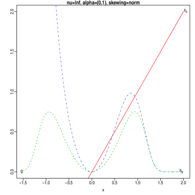
Figure 2: Case with $f_{0}=\phi$, $G_{0}=\Phi$ , $w(x)=x^{3}$. The left-side panel displays the functions $h_{0}$ (continuous), $g$ (dashed), $h_{g}$ (dot-dashed); the right-side panel displays $f(x)$

4 Quasi-concave and unimodal densities in $d$ dimensions

A real-valued function $f$ defined on a subset $S$ of $\mathbb{R}^{d}$ is said to be quasi-concave if the sets of the form $C_{u}=\{x:f(x)\geq u\}$ are convex for all positive $u$. If $d=1$, the notion of quasi-concavity coincides with uniqueness of the maximum, provided a pole is regarded as a maximum point, but for $d>1$ the two concepts separate. This motivates the following digression about concavity and related concepts, to develop some tools which will be used later on for our main target.

4.1 Concavity, quasi-concavity and unimodality

We first recall some standard notions available for instance in Chapter 16 of Marshall and Olkin (1979). A real function $f$ defined on a convex subset $S$ of $\mathbb{R}^{d}$ is said to be concave if, for every $x$ and $y\in S$ and $\theta\in(0,1)$, we have

$$f(\theta x+(1-\theta)y)\geq\theta f(x)+(1-\theta)f(y);$$

in this case $-f$ is a convex function. A function $f$ is said to be log-concave if $\log f$ is concave, that is for every $x$ and $y\in S$ and $\theta\in(0,1)$ we have

$$f(\theta x+(1-\theta)y)\geq f(x)^{\theta}f(y)^{1-\theta}.$$

The terms strictly concave and strictly log-concave apply if the above inequalities hold in a strict sense for all $x\neq y$ and all $\theta$.

Concave and log-concave functions defined on an open set are continuous. Moreover a twice differentiable function is concave (strictly concave) if and only if its Hessian matrix is negative semi-definite (negative definite) everywhere on $S$.

The next proposition provides the concave and log-concave extension of classical composition properties for convex functions such as statement (i) which can be found for example in Marshall and Olkin (1979, p. 451) together with its proof; the proofs of the other statements are completely analogous.

Proposition 10

Let $h$ be a real function defined on a convex set $S$, a subset of $\mathbb{R}^{d}$, and $H$ a monotone real function defined on a convex subset of $\mathbb{R}$, such that the composition $H(h)$ is defined on $S$. Then the following properties hold.

1. If $h$ is convex and $H$ non-decreasing and convex, then $H(h)$ is convex. Moreover $H(h)$ is strictly convex if $H$ is strictly convex, or if $h$ is strictly convex and $H$ is strictly monotone.

2. If $h$ is convex and $H$ non-increasing and log-concave, then $H(h)$ is log-concave. Moreover $H(h)$ is strictly log-concave if $H$ is strictly log-concave, or if $h$ is strictly convex and $H$ is strictly monotone. The same statements hold replacing the term log-concave by concave throughout.

3. If $h$ is concave and $H$ non-decreasing and log-concave, then $H(h)$ is log-concave. Moreover $H(h)$ is strictly log-concave if $H$ is strictly log-concave, or if $h$ is strictly concave and $H$ is strictly monotone. The same statements hold replacing the term log-concave by concave throughout.

We have defined quasi-concavity by requiring convexity of all sets $C_{u}$. An equivalent condition is that, for every $x$ and $y\in S\subseteq\mathbb{R}^{d}$ and $\theta\in(0,1)$, we have

$$f(\theta x+(1-\theta)y)\geq\min\{f(x),f(y)\}.$$

Obviously a function which is concave or log-concave is also quasi-concave. Similarly, both strict concavity and strict log-concavity imply strict quasi-concavity.

We now apply the above notions to the case where $f$ represents a probability density function on a set $S\subseteq\mathbb{R}^{d}$. The concept of unimodality has a friendly formal definition in the univariate case, see for instance Dharmadhikari and Joag-dev (1988, p .2), but this has has no direct equivalent in the multivariate case. Informally, we say that the term mode of a density refers to a point where the density takes a maximum value, either globally or locally. While a boring formal definition which allows for the non-uniqueness of the density function could be given, such a definition is not really necessary for the main aims of the present paper, since the density functions which we are concerned with are so regular that their modes are either points of (local) maxima or poles.

The set of the modes of a quasi-concave density is a convex set. Moreover, if $f$ is strictly quasi-concave, then the mode is unique. When the mode is unique we say that density $f$ is unimodal, and we say that $f$ is c-unimodal if the set of its modes is a convex set. If $X$ is a random variable with density function $f$ which is unimodal, we shall say that $X$ is unimodal, with slight abuse of terminology. The same convention is adopted for log-concavity, quasi-concavity and other properties.

Another important notion is $s$-concavity, which helps to make the concept of quasi-concavity more tractable. A systematic discussion of $s$-concavity has been given by Dharmadhikari and Joag-dev (1988); see specifically their Section 3.3, of which we now recall the main ingredients. Given a real number $s\neq 0$, a density is said to be $s$-concave on $S$ if

$$f(\theta x+(1-\theta)y)\geq\{\theta f(x)^{s}+(1-\theta)f(y)^{s}\}^{1/s}.$$

for all $x,\ y\in S$ and all $\theta\in(0,1)$.

Clearly, concavity corresponds to $s=1$. A density $f$ is $s$-concave with $s<0$ if and only if $f^{s}$ is convex; similarly, a density $f$ is $s$-concave with $s>0$ if and only if $f^{s}$ is concave. If we call ($-\infty$)-concave a function which is quasi-concave and $0$-concave a function which is log-concave, then the class of sets of $s$-concave functions is increasing when $s$ decreases; in other words, if $f$ is $s$-concave, then it is $r$-concave for any $r<s$. Finally, notice that is easy to adapt Proposition 10 to $s$-concave functions.

The closure with respect to marginalization of $s$-concave densities depends on the value of $s$ and on the dimensions of the spaces, as indicated by the next proposition, which essentially is Theorem 3.21 of Dharmadhikari and Joag-dev (1988).

Proposition 11

Let $f$ be an $s$-concave density on a convex set $S$ in $\mathbb{R}^{d+m}$, and $f_{d}$ be the marginal density of $f$ on an $d$-dimensional subspace. If $s\geq-1/m$, then $f_{d}$ is $s_{m}$-concave on the projection of the support of $f$, where $s_{m}=s/(1+ms)$, with the convention that, if $s=-1/m$, then $s_{m}=-\infty$.

Notice that this result includes the fact that the class of log-concave densities is closed with respect to marginalization. In addition, from a perusal of the proof of the above-quoted Theorem 3.21, we obtain that the marginal densities are strictly $s_{m}$-concave provided $f$ is strictly $s$-concave or the set $S$ is strictly convex.

4.2 Skew-elliptical distributions generated by conditioning

A $d$-dimensional random variable $U$ is said to have an elliptical density, with density generator function $\tilde{f}$, if its density $f_{U}$ is of the form

$$f_{U}(y)=k\,\tilde{f}(y^{\top}\Omega^{-1}y),$$ (16)

where $\Omega$ is a $d$-dimensional positive definite matrix, the function $\tilde{f}:(0,+\infty)\to\mathbb{R}^{+}$ is such that $x^{d/2-1}\tilde{f}(x)$ has finite integral on $(0,+\infty)$ and $k$ is a suitable constant which depends on $d$ and $\det(\Omega)$. In this case, we shall use the notation $U\sim\mathcal{E}_{d}(0,\Omega,\tilde{f})$.

Note that an elliptical density $f$ is c-unimodal if and only if its density generator is non-increasing, and it is unimodal if and only if its density generator is decreasing. Then it turn out that $f$ is c-unimodal if and only if it is quasi-concave, and it is unimodal if and only if it is strictly quasi-concave.

An initial formulation of skew-elliptical distribution has been considered by Azzalini and Capitanio (1999), which was of type (2) with $f_{0}$ of elliptical class and $w(x)$ linear. Another formulation of skew-elliptical distribution has been put forward by Branco and Dey (2001), whose key ingredients are now recalled. Consider a $(d+1)$-dimensional random variable

$$U=\pmatrix{U_{0}\cr U_{1}}\sim\mathcal{E}_{d+1}(0,\Omega_{+},\tilde{f})\,,\qquad\mathrm{where}\quad\Omega_{+}=\pmatrix{1&\delta^{\top}\cr\delta&\Omega}>0,$$ (17)

and $U_{0}$ and $U_{1}$ have dimension $1$ and $d$, respectively; for our aims, there is no loss of generality in assuming that the diagonal elements of $\Omega_{+}$ are all $1$’s. Then a random variable $Z=(U_{1}|U_{0}>0)$ is said to have a skew-elliptical distribution, and its density function at $u_{1}\in\mathbb{R}^{d}$ is

$$f_{Z}(u_{1})=2\int_{0}^{+\infty}k_{1}\tilde{f}(u^{\top}\Omega_{+}^{-1}{}u)\,\mathrm{d}u_{0}$$ (18)

where $u^{\top}=(u_{0},u_{1}^{\top})$. This construction arises as an extension of one of the mechanisms for generating the skew-normal distribution to the case of elliptical densities, but the study of the connections with other densities of type (2) was not an aim of Branco and Dey (2001).

Consequently, one question investigated by Azzalini and Capitanio (2003) was whether all distributions of type (18) are of type (2), with the requirement that $f_{0}$ is the density of an elliptical $d$-dimensional distribution. The conjecture has been proved for a set of important cases, notably the multivariate skew-normal and the skew-$t$ distributions, among others, but a general statement could not be obtained. This general conclusion is however quite simple to reach using representation (5), and recalling that Branco and Dey (2001) have proved that (18) can be written as

$$f_{Z}(y)=2\,\ f_{0}(y)\,F_{y}(\alpha^{\top}\,y),\qquad\qquad(y\in\mathbb{R}^{d}),$$ (19)

where $f_{0}$ is the density of an elliptical $d$-dimensional distribution, and $F_{y}$ is a cumulative distribution function of a symmetric univariate distribution, which depends on $y$ only through $y^{\top}\Omega^{-1}y$. Since $F_{y}=F_{-y}$, then it is immediate that $G(y)=F_{y}(\alpha^{\top}\,y)$ satisfies (4). Hence (19) allows a representation of type (5), and via (6) also of type (2).

Proposition 12

Assume that the random variable $U$ in (17) is c-unimodal. If $\tilde{f}$ is log-concave, then the elliptical densities of $U$ and $U_{1}$ and the skew-elliptical density of $Z$ are log-concave. Moreover they are strictly log-concave if $U$ is unimodal or $\tilde{f}$ is strictly log-concave or the support of $\tilde{f}$ is bounded.

Proof. Function $h(u)=u^{\top}\Omega_{+}^{-1}{}u$ is strictly convex. Since $U$ is c-unimodal, then $\tilde{f}$ is non-increasing, moreover it is log-concave; therefore $\tilde{f}(u^{\top}\Omega_{+}^{-1}{}u)$ is log-concave by Proposition 10 (ii). Then both $U$ and $(U|U_{0}>0)$ have log-concave densities. Since the marginals of a log-concave density are log-concave, then log-concavity of $U_{1}$ and $Z$ holds by (18). Now, if $U$ is unimodal, $\tilde{f}$ is decreasing, and $\tilde{f}(u^{\top}\Omega_{+}^{-1}{}u)$ is strictly log-concave, by Proposition 10 (i). If $\tilde{f}$ is strictly log-concave, then $\tilde{f}(u^{\top}\Omega_{+}^{-1}{}u)$ is strictly log-concave. Finally, if the support of $\tilde{f}$ is bounded, then the support of $U$ is strictly convex and, by Proposition 10 (i), also in this case $\tilde{f}(u^{\top}\Omega_{+}^{-1}{}u)$ is strictly log-concave. Then, in all three cases, strict log-concavity of $U_{1}$ and $Z$ holds by recalling the remark following Proposition 11.

This proposition is a special case of the more general result which follows, but we keep Proposition 12 separate both because of the special role of log-concavity and because this arrangement allows a more compact exposition of the combined discussion.

Proposition 13

Assume that the random variable $U$ in (17) is c-unimodal. If $\tilde{f}$ is $s$-concave, with $s\geq-1$, then $U$ has s-concave density, whereas the elliptical density of $U_{1}$ and the skew-elliptical density of $Z$ are $s_{1}$-concave, with $s_{1}=s/(1+s)$. Moreover all conclusions hold strictly if $U$ is unimodal or $\tilde{f}$ is strictly $s$-concave or the support of $\tilde{f}$ is bounded.

Proof. The function $h(u)=u^{\top}\Omega_{+}^{-1}{}u$ is strictly convex. Since $U$ is c-unimodal, then $\tilde{f}$ is non-increasing and moreover it is $s$-concave. We now examine properties of concavity separating the case $s<0$ and $s>0$; the case $s=0$, which corresponds to log-concavity, has already been handled in Proposition 12. If $s<0$ then $\tilde{f}^{s}$ is non-decreasing and convex. Then $\tilde{f}^{s}(u^{\top}\Omega_{+}^{-1}{}u)=\{\tilde{f}(u^{\top}\Omega_{+}^{-1}{}u)\}^{s}$ is convex by Proposition 10 (i) and $\tilde{f}(u^{\top}\Omega_{+}^{-1}{}u)$ is $s$-concave. On the other hand, if $s>0$ then $\tilde{f}^{s}$ is non-increasing and concave. Then $\tilde{f}^{s}(u^{\top}\Omega_{+}^{-1}{}u)=\{\tilde{f}(u^{\top}\Omega_{+}^{-1}{}u)\}^{s}$ is concave by Proposition 10 (ii) and $\tilde{f}(u^{\top}\Omega_{+}^{-1}{}u)$ is $s$-concave. Then both $U$ and $(U|U_{0}>0)$ have $s$-concave densities. Now, the claim about the densities of $U_{1}$ and $Z$ follows from Proposition 11 by taking into account (18). The final statement follows by the same type of argument used in the proof of Proposition 12.

Note that, in the special case of a concave density generator, the support is bounded, and both the marginal density on $\mathbb{R}^{d}$ and the skew-symmetric density of $Z$ are not necessarily concave. However, using Proposition 13 with $s=1$, strict $1/2$-concavity of their densities follows, and this fact implies strictly log-concavity.

The results of Proposition 12 and Proposition 13 allow to handle several classes of distributions, of which we now sketch the more noteworthy cases.

A important specific instance is the multivariate skew-normal density which can be represented by a conditioning method. For an expression of the multivariate skew-normal density, see for instance (16) of Azzalini (2005). Since the density generator of the normal family, $\tilde{f}(x)=\exp(-x/2)$, is decreasing and log-concave, then from Proposition 12 we obtain log-concavity of the skew-normal family. This conclusion is however a special case of a more general result on log-concavity of the SUN distribution obtained by Jamalizadeh and Balakrishnan (2010); see their Theorem 1.

The $(d+1)$-dimensional Pearson type II distributions for which $\tilde{f}(x)=(1-x)^{\nu}$, where $x\in(0,1)$ and $\nu\geq 0$, satisfies the conditions of Proposition 13. In fact it is non-increasing and $\nu^{-1}$-concave on a bounded support. Then the skew-elliptical $d$-dimensional density is strictly $(\nu+1)^{-1}$-concave and therefore strictly log-concave. The density function of the skew-type II density function is given by (22) of Azzalini and Capitanio (2003).

In addition, Proposition 13 holds for the Pearson type VII distributions, and in particular for the Student’s distribution. In this case the density generator is given by

$$\tilde{f}(x)=(1+x/\nu)^{-M}\qquad\qquad(\nu<0,\;(d+1)/2<M).$$ (20)

and $M=(d+\nu+1)/2$ for the Student’s density. Such generator is decreasing and $s$-concave with $s=-1/M$; in fact $\tilde{f}(x)^{-1/M}$ is convex. Since $s\geq-1$, then Proposition 13 applies and the skew-$t$ is $s_{1}$-concave with $s_{1}=-1/(M-1)$, and $s_{1}=-2/(d+\nu-1)$ in the Student’s case. These densities are not log-concave, but they are still strictly quasi-concave. Hence unimodality follows. For expressions of the multivariate skew-type VII and skew-$t$ density, see (21) and (26) of Azzalini and Capitanio (2003), respectively.

The above results establish not only unimodality of the more appealing subset of the skew-elliptical family of distributions, namely those of type (18), but also the much stronger conclusion of quasi-concavity of these densities. It is intrinsic to the nature of skew-elliptical densities that they do not have highest density regions of elliptical shape, but it is reassuring that they maintain a qualitatively similar behaviour, in the sense that convexity of these regions, $C_{u}$ in our notation, holds as long as the parent $(d+1)$-dimensional elliptical density enjoys a qualitatively similar property but in a somewhat stronger variant, specifically $s$-concavity with $s\geq-1$.

Note that there is no hope to extend Proposition 12 to quasi-concave densities, in the sense that a skew-symmetric generated by conditioning a quasi-concave density is not necessarily quasi-concave as demonstrated by the following construction.

Example

Consider $U=(U_{0},U_{1})^{\top}\sim\mathcal{E}_{2}(0,\Omega_{+},\tilde{f})$, where

$$\tilde{f}=I_{(0,1)}+I_{(0,4^{2})}\qquad\mathrm{and}\quad\Omega_{+}=\pmatrix{1&1/2\cr 1/2&1},$$

whose density function is

$$f_{U}(x,y)=k\{I_{S_{1}}(x,y)+I_{S_{4}}(x,y)\}$$

where $S_{j}=\{(x,y)\in\mathbb{R}^{2}:x^{2}+y^{2}-xy\leq 3j^{2}/4\}$, $j=1,4$, and $k$ is the normalizing constant given by $k=1/(A_{1}+A_{4})\approx 0.0216$ where $A_{j}=\pi\sqrt{3}j^{2}/2$ . Then both $U_{0}$, and $U_{1}$ have common support $[-4,4]$ and density function

$$f_{U_{0}}(x)=f_{U_{1}}(x)=k\,\left(\sqrt{3(1-x^{2})}\,I_{(-1,1)}(x)+\sqrt{3(16-y^{2})}\right)\,.$$

Because of (16) and (18), the density of $Z=(U_{1}|U_{0}>0)$ is given by

$$f_{Z}(y)=k\{f_{1}(y)+f_{4}(y)\}$$

where

$$f_{j}(y)=2\int_{0}^{+\infty}{I_{S_{j}}(x,y)}\,\mathrm{d}x=\cases{y+\sqrt{3(j^{2}-y^{2})}\quad&if $-\sqrt{3}j/2\leq y\leq\sqrt{3}j/2$,\cr 2\sqrt{3(j^{2}-y^{2})}&if $\sqrt{3}j/2\leq y\leq j$,\cr 0&otherwise,}\\$$

for $j=1,4$, and it is displayed in Figure 3. The global maximum of $f_{Z}$ is where $k(2y+\sqrt{3(16-y^{2})}+\sqrt{3(1-x^{2})})$ takes its maximum value, that is at $y\approx 0.699$. When $y>1$, $f_{Z}=kf_{4}$ and there is another local maximum at $y=2$. Therefore, $f_{Z}$ is not unimodal.

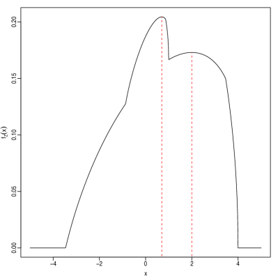
Figure 3: Density function $f_{Z}(x)$, exhibiting lack of quasi-concavity, obtained by conditioning of a bivariate elliptical quasi-concave distribution

To conclude with, while the density of $U$ is quasi-concave, the skew-elliptical variable $Z$ generated by conditioning is not quasi-concave.

4.3 Log-concavity of other families of distributions

There are several other families of distributions which belong to the area of interest of the stream of literature described at the beginning of this paper but are not included in the conditioning mechanism of an elliptical distribution considered in § 4.2. This section deals with log-concavity of some of these other families, making use of the following immediate implication of Proposition 10.

Corollary 14

If $q_{0}$ is a log-concave function defined on a convex set $S\subseteq\mathbb{R}^{d}$, and $H$ and $h$ are as in Proposition 10, either (ii) or (iii), then

$$q(x)=q_{0}(x)\,H\{h(x)\},\qquad(x\in S),$$ (21)

is log-concave on $S$.

Example

The density function on the real line introduced by Subbotin (1923) has been variously denoted by subsequent authors as exponential power distribution, generalized error distribution and normal distribution of order $\nu$. Its multivariate version is

$$f_{\nu}(x)=c_{\nu}\det(C)^{1/2}\,\exp\left(-\frac{(x^{\top}Cx)^{\nu/2}}{\nu}\right),\qquad(x\in\mathbb{R}^{d}),$$

where $C$ is a symmetric positive definite matrix, $\nu$ is a positive parameter and $c_{\nu}$ a normalization constant. For $\nu=2$ and $\nu=1$, $f_{\nu}$ lends the multivariate normal and the multivariate Laplace density, respectively.

We first want to show that $f_{\nu}$ is log-concave if $\nu\geq 1$. Consider $h(x)=(x^{\top}Cx)^{1/2}$ whose Hessian matrix is

$$\frac{\partial^{2}\,h(x)}{\partial x\>\partial x^{\top}}=h(x)^{-3}\left(x^{\top}CxC-Cxx^{\top}C\right)=h(x)^{-3}M,$$

say. To show that this Hessian is positive semi-definite, it is sufficient to prove this fact for matrix $M$, since $h(x)\geq 0$. For any $u\in\mathbb{R}^{d}$, write

$$u^{\top}Mu=(x^{\top}Cx)(u^{\top}Cu)-(u^{\top}Cx)(x^{\top}Cu)=\|\tilde{u}\|^{2}\,\|\tilde{x}\|^{2}-(\tilde{u}^{\top}\tilde{x})^{2}$$

where $\tilde{u}=C^{1/2}u$ and $\tilde{x}=C^{1/2}x$ for any square root $C^{1/2}$ of $C$, and from the Cauchy-Schwarz inequality we conclude that $u^{\top}Mu\geq 0$. Then $h$ is convex. Next, write

$$-\log f_{\nu}(x)=\mbox{constant}+h(x)^{\nu}/\nu$$

and observe that, since $t^{\nu}$ is a strictly convex for $t\geq 0$, then $-\log f_{\nu}$ is convex for $\nu\geq 1$ and strictly convex for $\nu>1$ by Proposition 10 (i). Hence $f_{\nu}$ is log-concave for $\nu\geq 1$ and strictly log-concave for $\nu>1$.

Now we introduce a skewed version of $f_{\nu}$ of type (2). If we aim at obtaining a density which fulfils the requirements of both Lemma 1 and Corollary 14, then $H=G_{0}$ is non-decreasing, while function $h=w$ must be odd and concave, hence it has to be linear. We then focus on the density function

$$f(x)=2\,f_{\nu}(x)\,G_{0}(\alpha^{\top}x),\qquad(x\in\mathbb{R}^{d}),$$ (22)

where $G_{0}$ is a distribution function on $\mathbb{R}$, symmetric about $0$.

Among the many options for $G_{0}$, a quite natural choice is to take $G_{0}$ equal to the distribution function of $f_{\nu}$ in the scalar case, that is

$$G_{0}(t)=\frac{1}{2}\left(1+\mathop{\rm sgn}\nolimits(t)\frac{\gamma(|t|^{\nu}/\nu,1/\nu)}{\Gamma(1/\nu)}\right)\,,\qquad t\in\mathbb{R},$$

where $\gamma$ denotes the lower incomplete gamma function. This choice of $G_{0}$ has been examined by Azzalini (1986) in the case $d=1$ of (22). He has shown that $G_{0}$ is strictly log-concave if $\nu>1$, leading to log-concavity of (22) when $d=1$. The case $\nu=1$ which corresponds to the Laplace distribution function is easily handled by direct computation of the second derivative to show strict log-concavity of $G_{0}$. Now, combining strict log-concavity of $G_{0}$ with log-concavity of $f_{\nu}$ proved above, an application of Corollary 14 shows that (22) is strictly log-concave on $\mathbb{R}^{d}$ if $\nu\geq 1$.

Although (22) is of skew-elliptical type, it is not of the type generated by the conditioning mechanism of a $(d+1)$-dimensional elliptical variate considered in Section 4.2. In fact, the results of Kano (1994) show that the set of densities $f_{\nu}$ is not closed under marginalization, and this fact affects the conditioning mechanism (18) as well.

As an example of non-elliptical distribution, we can consider a $d$-fold product of univariate Subbotin’s densities, that is

$$f_{\nu}^{*}(x)=\prod_{j=1}^{d}c_{\nu}\exp(-|x_{j}|^{\nu}/\nu)\,,\qquad x=(x_{1},\dots,x_{d})\in\mathbb{R}^{d}\,,$$

and this density can be used as a replacement of $f_{\nu}$ in (22). Since each factor of this product is log-concave, if $\nu\geq 1$, the same property holds for $f^{*}_{\nu}$. Strict log-concavity holds for $2f^{*}_{\nu}(x)G_{0}(\alpha^{\top}x)$ as well, using again strict log-concavity of $G_{0}$.

Example

To illustrate the applicability of Corollary 14 to distributions outside the set of type (2), consider the so-called extended skew-normal density which in the $d$-dimensional case takes the form

$$f(x)=\phi_{d}(x;\Omega)\,\frac{\Phi(\alpha_{0}+\alpha^{\top}\,x)}{\Phi(\tau)},\qquad\qquad(x\in\mathbb{R}^{d}),$$ (23)

where $\tau\in\mathbb{R}$ and $\alpha_{0}=\tau(\alpha^{\top}\Omega\alpha)^{1/2}$. Although this distribution does not quite fall under the umbrella of Lemma 1 unless $\tau=0$, its constructive argument is closely related.

To show log-concavity of (23), first recall the well-known fact that $\phi_{d}(x;\Omega)$ is strictly log-concave. Moreover $\Phi$ is log-concave, as if follows by direct calculation of the second derivative of $\log\Phi$, taking into account the well-known fact $-y\Phi(y)<\phi(y)$ for every $y\leq 0$. In addition, since $\Phi$ is strictly increasing and $\alpha_{0}+\alpha^{\top}\,x$ is concave in a non-strict sense, Corollary 14 applies to conclude that (23) is strictly log-concave.

Although this conclusion is a special case of the result of Jamalizadeh and Balakrishnan (2010) concerning log-concavity of the SUN distribution, it has however been presented because the above argument is different.

Acknowledgements

This research has been supported by MIUR, Italy, under grant scheme PRIN, project No. 2006132978.

References

- Azzalini (1985) Azzalini, A. (1985). A class of distributions which includes the normal ones. Scand. J. Statist. 12, 171–178.
- Azzalini (1986) Azzalini, A. (1986). Further results on a class of distributions which includes the normal ones. Statistica XLVI(2), 199–208.
- Azzalini (2005) Azzalini, A. (2005). The skew-normal distribution and related multivariate families (with discussion). Scand. J. Statist. 32, 159–188 (C/R 189–200).
- Azzalini and Capitanio (1999) Azzalini, A. and A. Capitanio (1999). Statistical applications of the multivariate skew normal distribution. J. R. Statist. Soc., ser. B 61(3), 579–602. Full version of the paper at arXiv.org:0911.2093.
- Azzalini and Capitanio (2003) Azzalini, A. and A. Capitanio (2003). Distributions generated by perturbation of symmetry with emphasis on a multivariate skew distribution. J. R. Statist. Soc., ser. B 65(2), 367–389. Full version of the paper at arXiv.org:0911.2342.
- Birnbaum (1948) Birnbaum, Z. W. (1948). On random variables with comparable peakedness. Ann. Math. Statist. 19, 76–81.
- Branco and Dey (2001) Branco, M. D. and D. K. Dey (2001). A general class of multivariate skew-elliptical distributions. J. Multivariate Anal. 79(1), 99–113.
- Capitanio (2008) Capitanio, A. (2008). On the canonical form of scale mixtures of skew-normal distributions. Unpublished manuscript.
- Dharmadhikari and Joag-dev (1988) Dharmadhikari, S. W. and K. Joag-dev (1988). Unimodality, Convexity, and Applications. New York & London: Academic Press.
- Genton (2004) Genton, M. G. (Ed.) (2004). Skew-elliptical Distributions and Their Applications: a Journey Beyond Normality. Chapman & Hall/CRC.
- Jamalizadeh and Balakrishnan (2010) Jamalizadeh, A. and N. Balakrishnan (2010). Distributions of order statistics and linear combinations of order statistics from an elliptical distribution as mixtures of unified skew-elliptical distributions. J. Multivariate Anal. to appear.
- Kano (1994) Kano, Y. (1994). Consistency property of elliptical probability density functions. J. Multivariate Anal. 51, 139–147.
- Ma and Genton (2004) Ma, Y. and M. G. Genton (2004). Flexible class of skew-symmetric distributions. Scand. J. Statist. 31, 459–468.
- Marshall and Olkin (1979) Marshall, A. W. and I. Olkin (1979). Inequalities: theory of majorization and its applications. Number 143 in Mathematics in Science and Engineering. New York & London: Academic Press.
- Serfling (2006) Serfling, R. (2006). Multivariate symmetry and asymmetry. In S. Kotz, N. Balakrishnan, C. B. Read, and B. Vidakovic (Eds.), Encyclopedia of Statistical Sciences (II ed.), Volume 8, pp. 5338–5345. J. Wiley & Sons.
- Subbotin (1923) Subbotin, M. T. (1923). On the law of frequency of error. Matematicheskii Sbornik 31, 296–301.
- Umbach (2006) Umbach, D. (2006). Some moment relationships for skew-symmetric distributions. Statist. Probab. Lett. 76(5), 507–512.
- Umbach (2008) Umbach, D. (2008). Some moment relationships for multivariate skew-symmetric distributions. Statist. Probab. Lett. 78(12), 1619–1623.
- Wang et al. (2004) Wang, J., J. Boyer, and M. G. Genton (2004). A skew-symmetric representation of multivariate distributions. Statist. Sinica 14, 1259–1270.