Towards holographic walking from ${\cal N}=4$ super Yang-Mills

Abstract

We propose that a holographic description of ‘walking’ behaviour, namely quasi-conformal dynamics relevant for technicolor models, can be obtained from relevant deformations of ${\cal N}=4$ super Yang-Mills. We consider deformations which drive the theory close to the ${\cal N}=1$ Leigh-Strassler fixed point, eventually deviating from it in the deep IR. We use the Pilch-Warner dual supergravity description of the flow between the ${\cal N}=4$ and the ${\cal N}=1$ fixed points to focus on observables that only require knowledge of the walking region. These include large anomalous dimensions of quark bilinear operators, which we study via probe D7-branes. We also make a first attempt at describing the theory beyond the walking region by introducing an infrared cut-off, in the spirit of hard-wall models. In this case we find a light, dilaton-like scalar state, but whether this mode persists in the exact theory remains an open question.

ICCUB-10-203

1 Introduction

Walking technicolor (WTC) WTC is an appealing candidate for dynamical electro-weak symmetry breaking (EWSB) (see reviews ; P for reviews on the topic). The basic idea is that EWSB may be triggered by the formation of a non-trivial condensate due to a new strongly-coupled interaction, along the lines of technicolor (TC) TC . What makes WTC special is that, in addition to being strongly coupled, the underlying dynamics is assumed to be approximately conformal over a range of energies above the electro-weak scale, and in this range large anomalous dimensions are present. This improves on some of the difficulties of traditional TC models, as we review in Section 2. In view of the recently-started LHC program, it is important to identify clear experimental signatures distinguishing this type of proposal from weakly-coupled theories, such as the minimal version of the Standard Model or its supersymmetric extensions.

Unfortunately, the strongly-coupled nature of WTC makes its study by conventional field theory methods (based on perturbation theory) difficult, and many non-trivial field theory questions remain open. One important such question is whether in a WTC model, due to the spontaneous breaking of dilatation symmetry induced by the EWSB condensate, there exists a light scalar composite state with the properties of a light dilaton. If so, this field would have a phenomenology very similar to that of the light Higgs in the minimal version of the standard model dilaton ; dilatonpheno ; dilaton2 ; dilaton5D .

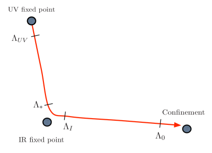
Aside from its potential phenomenological implications, the question about the existence of a light dilaton is of intrinsic interest from a purely field-theoretical viewpoint. Indeed, consider a four-dimensional quantum field theory whose renormalization group (RG) flow is characterized by three dynamically generated scales $\Lambda_{0}<\Lambda_{I}<\Lambda_{\ast}$, as sketched in figure 1, with the the following properties.

Figure 1: Left: RG flow of a walking theory. Right: Cartoon of the effective gauge coupling $g$ as a function of the renormalization scale $\mu$.

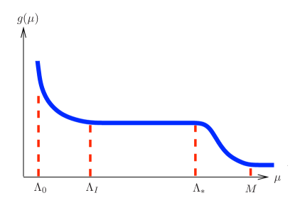The theory is UV-complete, in the sense that at energies above some high scale $\Lambda_{UV}$ the dynamics is governed by a (possibly interacting) UV fixed point, from which the flow is driven away by some relevant operator. For example, in pure Yang-Mills theory the gauge coupling itself represents a (marginally) relevant deformation driving the theory away from the UV fixed point, which is free in this case. Following the RG flow towards lower energies, there exists another fixed point, which we will refer to as an IR fixed point. The flow is attracted towards this fixed point at energies below $\Lambda_{\ast}$, but does not reach the fixed point and is driven away at energies below $\Lambda_{I}$. In the energy region $\Lambda_{I}<E<\Lambda_{\ast}$ the theory is almost scale-invariant and is approximately described by the conformal field theory (CFT) living at the IR fixed point; in particular, coupling constants stop running almost completely. Generically, the operators in this CFT have dimensions completely different from those at the UV fixed point, and hence in matching the descriptions along the flow one will find that large, non-perturbative anomalous dimensions have emerged. Note that, despite the appearance of figure 1(left), if the flow comes very close to the IR fixed point then a large hierarchy $\Lambda_{I}\ll\Lambda_{\ast}$ develops, as shown in figure 1(right). There may or may not be a tunable parameter that controls the size of this hierarchy. Below $\Lambda_{I}$ the flow just drifts away from the IR fixed point and the theory ultimately confines at some lower scale $\Lambda_{0}$. With some abuse of terminology, in the following we will call a theory with these properties a ‘walking theory’ — walking technicolor is an example of such a theory, in which at some scale $\Lambda_{W}\in[\Lambda_{0},\Lambda_{I}]$ a condensate forms, spontaneously breaking the $SU(2)_{L}\times U(1)_{Y}$ symmetry of the Standard Model.

In a scenario like the above, one question we would eventually like to address is: Under what conditions, for example on the anomalous dimensions of operators at the IR fixed point, does the spectrum contain a scalar composite state with the quantum numbers and the couplings of a dilaton and a mass parametrically lighter than the mass gap $\Lambda_{0}$. In order to pose this question, one first needs to construct a model with the properties of a walking theory, and in order to address the question one then needs to find an appropriate tool to study the strong coupling dynamics. In this paper we propose that certain relevant deformations of ${\cal N}=4$ super Yang-Mills (SYM) theory can provide such models, and that their dual string descriptions provide such tools, at least in principle.

Previous steps towards the construction of a walking theory in the context of the gauge/string duality AdSCFT (see reviewAdSCFT for a review) were given in NPP ; NPR ; ENP . By wrapping D5-branes on a two-sphere as in MN , these references constructed supergravity solutions that exhibit some of the features expected of a walking theory. In particular, a suitably-defined gauge coupling exhibits slow running in a strongly-coupled IR region, and even more deeply in the IR the theory confines NPR . Moreover, ref. ENP found evidence of the presence in the spectrum of an anomalously light scalar with a mass suppressed by the length of the walking region. The calculation of the spectrum was greatly facilitated by the use of a gauge-invariant formalism BHM .

Despite the appealing features of these models, two obstacles are encountered when attempting to establish the properties of the light scalar that are necessary for its identification as a light dilaton. First, although in the walking region the gauge coupling and many other dynamical quantities become effectively constant, the background metric is not approximately AdS, so a direct connection with some approximate conformal symmetry is not apparent. Second, a direct calculation of the couplings of the light scalar is difficult because in the far-UV the geometry is not asymptotically AdS either, and hence the rigorous procedure of holographic renormalization cannot be straightforwardly applied.

We propose that these two difficulties can be overcome in principle by constructing a walking theory as a relevant deformation of ${\cal N}=4$ SYM. From the above discussion it is evident that the main necessary ingredient is the existence of a flow between two conformal field theories, where the IR fixed point theory is strongly interacting. In addition, we require that the flow between the two CFT’s have a dual supergravity description which provides the requisite tool for extracting quantitative results at strong coupling. The simplest such flow is the one from ${\cal N}=4$ SYM to the ${\cal N}=1$ supersymmetric Leigh-Strassler fixed point (LS FP). In ${\cal N}=1$ language, the ${\cal N}=4$ theory contains a vector superfield and three chiral superfields $\Phi_{i}$. When deformed by a relevant operator corresponding to a mass $m_{3}$ for one of these chiral superfields, say $\Phi_{3}$, it is known that the ${\cal N}=4$ theory flows to a strongly interacting ${\cal N}=1$ SCFT, first identified by Leigh and Strassler LS .

The five-dimensional supergravity solution dual to the LS FP was found in KPW (see also 5d ). The ten-dimensional supergravity solution describing the entire LS flow between the UV and the IR fixed points was found by Pilch and Warner PW by uplifting the five-dimensional flow of FGPW . As we will review, the PW flow is described by a completely smooth supergravity solution that is known in closed form for all practical purposes.

Given the flow between two supersymmetric fixed points it is possible to arrange a situation where the theory enters a walking regime. This is achieved by further deforming the flow by a set of ${\cal N}=1$ chiral operators ${\cal O}_{i}$ (superpotential deformations) which are relevant at the IR fixed point, with a corresponding set of couplings ${h_{i}}$:

$${\cal L}_{{\cal N}=4}\,\,\to\,\,{\cal L}_{{\cal N}=4}+\int d^{2}\theta\,\left(m_{3}{\rm Tr}\Phi_{3}^{2}+\sum h_{i}{\cal O}_{i}\,\right)+\,h.c.$$ (1)

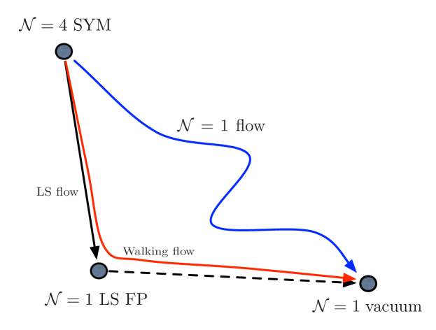
We focus on supersymmetric deformations for the usual reasons of technical convenience, but non-supersymmetric deformations could just as well be considered. Assuming that the deformed theory has at least one isolated, supersymmetric ground state ${\cal G}$, one can always choose the couplings $h_{i}$ to be parametrically small so the flow gets as close as possible to the LS fixed point, before the relevant operators ${\cal O}_{i}$ drive the theory to the IR vacuum ${\cal G}$. The idea is summarized in figure 2.

Figure 2: RG flows from the ${\cal N}=4$ SYM theory: The continuous black line describes the flow between the UV fixed point and the IR ${\cal N}=1$ Leigh-Strassler fixed point, induced by turning on $m_{3}\neq 0$. The blue curve describes an ${\cal N}=1$ flow induced by turning on, in addition to $m_{3}$, operators that remain relevant in the IR. The red curve corresponds to an ${\cal N}=1$ flow, for some choice of relevant couplings, which just misses the LS fixed point.

The above scenario is quite general and it is useful to have an illustrative example at hand, although we do not wish to restrict attention solely to it. Such an example is provided by the ${\cal N}=1^{*}$ deformation of the ${\cal N}=4$ theory, wherein we introduce masses $m_{i}$ for each of the $\Phi_{i}$. The set of vacua of this theory is well understood on field-theoretic grounds dw ; dorey ; doreykum , and is known to include confining vacua. A specific pattern of masses such that $m_{1}=m_{2}=m$ and $m_{3}=\Lambda_{UV}$, with $m\ll\Lambda_{UV}$, realizes the desired walking scenario discussed above. Since the flow ends exactly at the LS FP in the case in which $m=0$, it must pass close to the FP if $m\ll\Lambda_{UV}$. In this case, the extent of the walking region is controlled by the tunable parameter $m/\Lambda_{UV}$. This shows that, in principle, deformations of ${\cal N}=4$ SYM can furnish examples of walking theories in which to pose some of the questions discussed above.

However, it is not a priori clear which deformations among those that exhibit walking behaviour also yield a light scalar to be identified as a pseudo-dilaton. The answer to this question depends on the dynamical details, and for this reason the first steps that we will take in this paper will not be tied to a specific deformation of the LS flow.

Changing the coupling constant in ${\cal N}=4$ SYM is an exactly marginal deformation, so one can choose the UV fixed point to be weakly or strongly coupled. Regardless of this choice, however, the theory in the vicinity of the IR fixed point and beyond is inevitably strongly coupled. While field-theoretic methods may still be useful to study some aspects of the dynamics in this regime (e.g. the calculation of condensates of chiral operators), other aspects require a different method. These include, for example, the calculation of the anomalous dimensions of some operators in the vicinity of the LS FP or the existence of a light dilaton.

In this paper, we will use the dual string description of the flow from the ${\cal N}=4$ theory to the Leigh-Strassler SCFT, due to Pilch and Warner, to address some of these questions. We will focus on questions that can be answered using only our knowledge of the Pilch-Warner solution. In particular, we will not address the string dual description of the relevant deformations that take the theory away from the LS fixed point.

Our main results are contained in Sections 5 and 6. In Section 5 we will determine the anomalous dimensions of operators of interest in the walking region and compare them to the corresponding dimensions at the UV FP. We emphasize that this calculation does not require knowledge of the string dual of the entire LS flow but only of the LS FP itself. For this reason, the results of this calculation will apply to any deformation of the LS flow that one may wish to consider. The operators we consider include quark bilinears, which we describe as fields on probe D7-branes. In Section 6 we turn to the existence of a light dilaton in the spectrum. Addressing this question rigorously does require knowledge of the string dual of the entire flow (inlcuding the dynamics that drives the theory out of the LS fixed point), which is not presently available. In order to circumvent this difficulty, we introduce UV and IR cut-offs on the PW solution. The UV cut-off is a technical convenience and it could be removed. The idea behind the IR cut-off is that the first part of the flow we are interested in, represented by the first part of the red curve in figure 2, including the walking region, is well approximated by the LS flow. Cutting-off this solution in the IR is therefore a crude attempt at modeling, in the spirit of hard-wall models hardwall , the true dynamics that eventually leads to confinement in the deformations of ${\cal N}=4$ SYM of the kind described above. Although we find a light composite state in the spectrum whose mass scales with the size of the walking region as expected for a light dilaton, we also emphasize that whether this state persists in the exact theory remains an open question. In Section 7 we discuss possible future directions to address this question in the exact theory.

The reader familiar with the necessary background can safely skip to Section 5. However, we have included some additional sections for the benefit of the unfamiliar reader. In Section 2 we review relevant aspects of WTC. We emphasize the motivation for the several scales $\Lambda_{0}\mathrel{\raisebox{-2.58334pt}{$\stackrel{{\scriptstyle\textstyle<}}{{\sim}}$}}\Lambda_{W}\mathrel{\raisebox{-2.58334pt}{$\stackrel{{\scriptstyle\textstyle<}}{{\sim}}$}}\Lambda_{I}\ll\Lambda_{\ast}$ and for our focus on the walking region $\Lambda_{I}<\mu<\Lambda_{\ast}$. In Section 3 we review several aspects of the ${\cal N}=4$ theory and its deformations, and we elaborate on the walking scenario discussed above. In Section 4 we review the supergravity description of the LS flow. This section also contains a Wilson-loop calculation of the quark-antiquark potential along the flow that has not appeared before. Some technical details have been relegated to the Appendices.

2 Walking technicolor

In this brief section we remind the reader about why WTC is an interesting alternative to weakly-coupled models of EWSB. In particular, we want to summarize the reasons why we are interested in a theory that has several separated scales ($\Lambda_{0}\mathrel{\raisebox{-2.58334pt}{$\stackrel{{\scriptstyle\textstyle<}}{{\sim}}$}}\Lambda_{W}\mathrel{\raisebox{-2.58334pt}{$\stackrel{{\scriptstyle\textstyle<}}{{\sim}}$}}\Lambda_{I}\ll\Lambda_{\ast}$), why we would like it to be quasi-conformal in the range $\Lambda_{I}<\mu<\Lambda_{\ast}$ (the walking region), and why we want large anomalous dimensions in this range. We dispense with specifying any details of the microscopic realization of WTC because, since they only affect the physics above the scale $\Lambda_{\ast}$, they are irrelevant for the arguments presented here. Much more extensive and detailed discussions can be found elsewhere reviews ; P . In reading this section, one should remember that in this paper we are mostly concerned with the physics taking place in the walking region. It should also be kept in mind that many observables in the context of dynamical EWSB (technicolor) are hard to calculate using conventional methods because of the associated strong interactions. For this reason, most of the general arguments we summarize here are based on order-of-magnitude estimates.

The basic idea of TC is to replace the Higgs sector of the SM by a completely new, strongly-coupled interaction (called ‘techni-colour’ after the colour interaction of QCD) together with a corresponding set of new degrees of freedom (techni-quarks $Q$, techni-mesons $M$, techni-baryons $B$, etc). This strongly-coupled theory will in general have some large internal global symmetry $G_{f}$, spontaneously broken by the formation of condensates triggered by the strong interaction itself to some subgroup $G_{f}\rightarrow H_{f}$. By identifying an $SU(2)\times U(1)\subset G_{f}$ subgroup of such a global symmetry with the electro-weak gauge symmetry, one can induce EWSB provided $H_{f}\cap(SU(2)\times U(1))=U(1)$, with the latter being the $U(1)$ associated to electromagnetism.

Let us therefore start from low energies and motivate, on phenomenological grounds, the requirements we wish to impose on the strongly coupled theory. In doing so we will provide a physical meaning for each of the four dynamical scales in the theory. The first condition is that the theory should not contain experimentally-unobserved light states that couple to the SM. The scale $\Lambda_{0}$ at which the theory confines must therefore provide a mass gap that is large enough to evade all direct searches for new (techni-)particles.

The scale $\Lambda_{W}$ is the characteristic scale of the condensate that breaks spontaneously the $SU(2)\times U(1)$ symmetry. In principle, this might simply be the scale $\Lambda_{0}$ itself, as in QCD, but this need not be the case in general. The physics of precision parameters, most importantly $\hat{S}$ PT ; Barbieri , is controlled by $\Lambda_{W}/\Lambda_{0}$ and by model-dependent, hard-to-calculate coefficients. Hence one should consider $\Lambda_{W}$ and $\Lambda_{0}$ as independent, though not necessarily parametrically separated, parameters.

A serious phenomenological problem of TC is that one also has to implement a mechanism that provides a mass for the SM fermions $f$. In the absence of a Higgs field, the operator of lowest dimension that can provide such a mass is of the form ${\cal O}_{6}=\bar{f}f\bar{Q}Q$, which on the basis of naive power counting is highly irrelevant. This produces two problems. First of all, if one wants to have a UV-complete theory, one has to provide an origin for such an operator. This is achieved by embedding TC into extended technicolor (ETC) ETC , the basic idea of which is to unify the family symmetries of the SM and the gauge symmetry of TC into a strongly coupled theory. In this theory, symmetry-breaking yields, below some scale $\Lambda_{ETC}$, an effective theory consisting of TC and a series of higher-order operators such as ${\cal O}_{6}$ coupling TC fermions and SM fermions.

At this point one is left with a second, even more serious problem, which is the reason why walking enters into the game. In implementing ETC, one also produces 4-fermion operators of the form $\bar{f}f\bar{f}f$. These involve SM fermions only, and therefore contribute directly to FCNC processes. Finding a model of ETC that avoids inducing excessively-large contributions to FCNC processes is tightly bound within the search for models that explain the large hierarchies between SM fermion masses. For the most part this search reduces to a non-trivial exercise in model building, in which one constructs (tumbling) multi-scale ETC models that implement a mild version of the Glashow-Iliopoulos-Maiani (GIM) suppression (see for instance APS ). What is unavoidable, though, is the (indirectly related) fact that a new-physics source of contributions to the $\hat{T}$ precision parameter PT ; Barbieri is introduced at the lightest ETC scale, which contains the dynamical origin of the huge top-bottom mass splitting. Ultimately, this means that one must at least require that all ETC scales be larger than the bound deduced via naive dimensional analysis from $\hat{T}$: $\Lambda_{ETC}\geq\Lambda_{\ast}\mathrel{\raisebox{-2.58334pt}{$\stackrel{{\scriptstyle\textstyle>}}{{\sim}}$}}5$ TeV.

There is hence a scale separation $\Lambda_{W}\ll\Lambda_{\ast}$. If naive dimensional analysis were to apply, this would mean that the mass of the top quark should be $m_{t}\sim\Lambda_{W}^{3}/\Lambda_{\ast}^{2}$, and it would be impossible to justify the experimental fact that actually $m_{t}\sim{\cal O}(\Lambda_{W})$. Walking overcomes this difficulty: if the TC theory, for energies below $\Lambda_{\ast}$, is very close to an approximate fixed point, all the operators will inherit their dimensionality not from the naive counting, but rather from the dimensions of the CFT living at the fixed point. Hence, large anomalous dimensions are expected, affecting all the physical quantities important at long distances, and the scaling of the mass of the top would be $m_{t}\sim\Lambda_{W}^{3}/\Lambda_{\ast}^{2}\times(\Lambda_{\ast}/\Lambda_{W})^{-\gamma}$, with $\gamma$ the anomalous dimension of the chiral condensate. In this way, large masses for the top can be accommodated, and the basic phenomenology of the SM is successfully reproduced.

As stated above, in the deep IR the theory must confine and break chiral symmetry. A conformal theory cannot do so. It must hence be the case that some physical effect yields breaking of scale invariance characterized by a scale $\Lambda_{I}\ll\Lambda_{\ast}$, so that the theory is approximately scale invariant only in the (walking) region $\Lambda_{I}<\mu<\Lambda_{\ast}$. It is usually assumed that $\Lambda_{I}=\Lambda_{W}$. Again, it is clear that there is some relation between $\Lambda_{0}$, $\Lambda_{W}$ and $\Lambda_{I}$, but in general there is no obvious reason why they must coincide. Hence one should treat $\Lambda_{I}$ as an independent scale, requiring only that $\Lambda_{0}\leq\Lambda_{W}\leq\Lambda_{I}$.

Walking technicolor has also another, less explored but possibly even more important consequence. While ETC has a very large gauge symmetry but a limited amount of global symmetry, below $\Lambda_{\ast}$ the resulting TC model typically has very large global symmetries (typical QCD-like examples yield at least an $SU(8)_{L}\times SU(8)_{R}$ symmetry), which are broken only by the higher-order operators of the form $\bar{Q}Q\bar{Q}Q$ arising at or above the scale $\Lambda_{\ast}$. If there were no large anomalous dimensions, this would immediately imply the presence of large numbers of pseudo-Nambu-Goldstone bosons (techni-pions or techni-axions) due to the spontaneous breaking of the global symmetry (see for instance AW ). Some of them would carry electro-weak interactions and have typical masses in the GeV-range, well below the experimental exclusion bounds, thus invalidating the whole model. However, because of the same arguments as for the top quark, the large anomalous dimensions could enhance these masses above the experimental bounds. Furthermore, one might even speculate that the presence of such higher-order operators might play a role in the very mechanism leading the theory away from the IR fixed point, and ultimately towards confinement and chiral-symmetry breaking.

To summarize, a generic TC theory potentially suffers from four phenomenologically unacceptable features which, in order of severity, are: (i) A tension between the heavy mass of the top and the smallness of the $\hat{T}$ parameter; (ii) the presence of very light techni-pions; (iii) large contributions to precision parameters such as $\hat{S}$; and (iv) a potential problem in identifying an ETC model that explains the SM-fermion mass hierarchies while suppressing FCNC. Avoiding all of these severely restricts the viable candidates. WTC is one such candidate characterized by at least the four scales $\Lambda_{0}\leq\Lambda_{W}\leq\Lambda_{I}\ll\Lambda_{\ast}$ and by the presence of large anomalous dimensions in the range $\Lambda_{I}<\mu<\Lambda_{\ast}$. All the ETC physics takes place above the scale $\Lambda_{\ast}$ and is of no concern for this paper. Rather, our more restricted goal is the study of a model whose dynamics in the energy range $\Lambda_{I}<\mu<\Lambda_{\ast}$ is quasi-conformal and strongly-coupled, so that large, non-perturbative anomalous dimensions are present. In particular, this means that we will not discuss the physics below the scale $\Lambda_{I}$ either, and hence we can (for the time being) ignore completely electro-weak symmetry breaking and confinement.

We close this section by reminding the reader that an active program is underway in the context of lattice field theory — see e.g. lattice and references therein. The numerical study of a large class of gauge theories with various field contents aims at (i) identifying precisely the conditions under which a theory exhibits conformal or quasi-conformal (walking) behavior in the IR, and (ii) studying in such models physical observables such as mass spectra, anomalous dimensions, etc. Proposals such as ours provide a complementary, analytical approach in which similar questions can be posed and addressed.

3 Walking from deformations of ${\cal N}=4$ SYM

A natural setting for investigating the walking scenario described above, within a potentially consistent holographic framework, is provided by certain relevant deformations of ${\cal N}=4$ supersymmetric $SU(N)$ gauge theory which drive the theory arbitrarily close to a non-trivial conformal fixed point at low energies. The essential idea is to consider an ${\cal N}=1$ supersymmetric deformation of the ${\cal N}=4$ UV fixed point, such that deep in the IR the theory confines with a mass gap, whilst at intermediate energy scales the theory exhibits ‘almost conformal’ behaviour as it stays in the vicinity of an ${\cal N}=1$ superconformal fixed point. The ${\cal N}=1$ fixed point in question is the one discovered by Leigh and Strassler LS , which we review below. For this discussion, it is convenient to view the ${\cal N}=4$ theory as consisting of an ${\cal N}=1$ vector multiplet ${\cal W}_{\alpha}$ and three adjoint chiral multiplets $\Phi_{a}$, $a=1,2,3$. The superpotential of the theory is

$$W_{{\cal N}=4}=-{\tau\over 16\pi i}{\rm Tr}\left({\cal W}_{\alpha}^{2}\right)+\frac{1}{g^{2}_{\textrm{\tiny YM}}}{\rm Tr}\left(\Phi_{3}[\Phi_{1},\Phi_{2}]\right),$$ (2)

where

$$\tau=\frac{4\pi i}{g^{2}_{\textrm{\tiny YM}}}+\frac{\theta}{2\pi}$$ (3)

is the complexified gauge coupling. In this picture, an $SU(3)\times U(1)$ subgroup of the full $SU(4)$ R-symmetry of the ${\cal N}=4$ theory is manifest.

The addition of a supersymmetric mass term for one of the chiral multiplets,

$$\Delta W=\frac{1}{2g^{2}_{\textrm{\tiny YM}}}\,m_{3}{\rm Tr}\Phi_{3}^{2}\,,$$ (4)

makes the ${\cal N}=4$ theory flow to a strongly interacting ${\cal N}=1$ SCFT in the IR LS . Integrating out the massive field for energies below $m_{3}$ yields the quartic superpotential

$$W=-\frac{\tau}{16\pi i}{\rm Tr}{\cal W}_{\alpha}^{2}-\frac{1}{m_{3}\,g^{2}_{\textrm{\tiny YM}}}{\rm Tr}[\Phi_{1},\Phi_{2}]^{2}.$$ (5)

Following the arguments of LS ; ails , in the deep infrared this theory flows to a fixed point wherein the anomalous dimension of each of the two light adjoints is $\gamma_{\phi}=-1/4$ and the quartic superpotential is actually an exactly marginal operator — we define the anomalous dimension of an operator with canonical dimension $d$ as $\Delta=d+\gamma_{\phi}$, where $\Delta$ is the scaling dimension in the IR. The corresponding marginal coupling inherits the $SL(2,{\mathbb{Z}})$ duality property of the gauge coupling of the ‘parent’ ${\cal N}=4$ gauge theory ails . The presence of the two massless adjoint chiral multiplets implies that the theory, and in fact the entire flow from ${\cal N}=4$ SYM to the IR SCFT, has an $SU(2)\times U(1)_{R}$ global symmetry. The $U(1)_{R}$ factor is identified with the non-anomalous R-symmetry of the IR ${\cal N}=1$ SCFT. In view of (5) the scalar fields $\Phi_{1,2}$ must each carry R-charge $R=+1/2$ at the fixed point, so that the R-charge of the superpotential is $R=2$. The ${\cal N}=1$ superconformal algebra then fixes the scaling dimension of all chiral operators in terms of their R-charges as

$$\Delta=\frac{3}{2}\,|R|\,.$$ (6)

It follows that all supersymmetry-preserving relevant defomations (F-terms) can also be identified at the Leigh-Strassler fixed point. These include single-trace operators which are quadratic and cubic in the fields, such as ${\rm Tr}\Phi_{1}^{2}\,,{\rm Tr}\Phi_{1}\Phi_{2}\,,{\rm Tr}\Phi_{1}^{2}\Phi_{2}$, etc. Chiral operators which are quartic in the scalar fields will be marginal at the fixed point, and some of them could be marginally relevant.

The theory below the scale $m_{3}$ is $SU(N)$ pure ${\cal N}=1$ SYM coupled to two adjoint chiral multiplets. This theory by itself is asymptotically free, but in our construction it matches on to ${\cal N}=4$ SYM at the scale $m_{3}$. Above that scale the presence of the third chiral multiplet makes the theory conformal. Since the theory below the scale $m_{3}$ is asymptotically free, it must become strongly coupled at a dynamically-generated scale $\Lambda_{\ast}\leq m_{3}$. In general, the relationship between these two scales receives (unknown) instanton contributions and takes the form

$$\Lambda_{\ast}^{N}=m_{3}^{N}f(q)\,,\qquad\mbox{with }q=e^{2\pi i\tau}\,.$$ (7)

However, if the ${\cal N}=4$ ’t Hooft coupling is weak, i.e. if $g_{\textrm{\tiny YM}}^{2}N\ll 1$, then $f(q)=q+\cdots$ ails . Assuming for simplicity that the theta-angle vanishes this immediately implies the more familiar relation

$$\Lambda_{\ast}\sim m_{3}\;e^{2\pi i\tau/N}\sim m_{3}e^{-8\pi^{2}/g_{\textrm{\tiny YM}}^{2}N}\,.$$ (8)

We expect the theory to flow to the IR CFT only below the scale $\Lambda_{\ast}$ ails . The existence of the IR fixed point itself is inferred from the exact beta-functions for the gauge coupling and the coefficient of the quartic superpotential. We may now consider additional perturbations of the theory by operators which are relevant at the IR fixed point,

$$W\to W+\sum_{i}h_{i}{\cal O}_{i}\,,$$ (9)

such that the scales associated to the dimensionful couplings $h_{i}$ are much smaller than $\Lambda_{*}$. The theory will then be quasi-conformal for a large range of energies below $\Lambda_{*}$, until the effect of the relevant couplings $h_{i}$ becomes important and drives the theory to a vacuum with a mass gap (for a suitable choice of operators ${\cal O}_{i}$).

As we have already seen in Section 1, the simplest example of this situation occurs in the mass deformation of ${\cal N}=4$ SYM that incorporates masses $m_{1},m_{2},m_{3}$ for all three chiral multiplets, such that $m_{1}=m_{2}=m\ll\Lambda_{\ast}$, which would leave the theory looking conformal for all energy scales $\Lambda_{I}<\mu<\Lambda_{\ast}$. Here $\Lambda_{I}\propto m$ with a constant of proportionality that can, in principle, be a non-trivial function of the marginal coupling characterizing the ${\cal N}=1$ fixed point. The deformation of the ${\cal N}=4$ theory by three supersymmetric non-zero mass terms is also known as the ${\cal N}=1^{*}$ theory. When the scalar VEVs in the field theory vanish, the IR dynamics of the theory is qualitiatively similar to pure ${\cal N}=1$ SYM theory in that a mass gap and a gluino condensate are dynamically generated. For weak UV ’t Hooft coupling $g_{\textrm{\tiny YM}}^{2}N\ll 1$, the strong coupling scale $\Lambda_{0}=(m^{2}m_{3})^{1/3}\,e^{2\pi i\tau/3N}$ will be lower than $\Lambda_{I}\sim m$, so that the confining scale is separated from the walking regime. The vacuum and phase structure, as well as the corresponding chiral condensates, can all be determined precisely dw ; dorey ; doreykum ; adk ; mm and their functional forms depend in a rather simple way on the mass parameters $m_{i}$. The main point we want to make here is that the ${\cal N}=1^{*}$ theory in the limit $m\ll m_{3}$ provides a realization of the walking scenario we have described. We will come back to this point in Section 7.

We also emphasize, however, that ${\cal N}=1^{*}$ should be viewed as just one example within a wider class of theories that realize the walking dynamics that we are interested in. Other examples include cubic- and perhaps quartic-superpotential deformations of ${\cal N}=4$ SYM (always accompanied by a large mass $m_{3}$) which remain relevant or marginally relevant at the Leigh-Strassler fixed point. A detailed study of the vacuum structure and condensates of such deformations would be extremely interesting to pursue, but is beyond the scope of the present discussion.

4 Supergravity description of the Leigh-Strassler flow

In this section we first review the basic setup of the dual supergravity description of the flow from ${\cal N}=4$ SYM to the LS ${\cal N}=1$ SCFT, which is applicable at strong coupling and large $N$. This includes the five-dimensional supergravity sigma-model and its uplift to ten dimensions as proposed by Pilch and Warner PW . Next we discuss in some detail the space of all possible solutions to the BPS equations of the system, by mapping out and characterizing the flows in terms of the positions of all the fixed points and singularities. To some extent, the content of this analysis is already known in the literature, and can be summarized by saying that out of all possible solutions to the background equations, only a one-parameter family is fully acceptable on physical grounds. This family corresponds to solutions that exactly interpolate between the ${\cal N}=4$ and the LS fixed points. We find it useful to summarize these results for the sake of completeness and also to fix notation. Finally, we examine properties of the flow towards the fixed points by using Wilson lines to probe the IR geometry.

4.1 The five-dimensional supergravity sigma-model

We start from the $SU(2)\times U(1)$-invariant truncation of five-dimensional ${\cal N}=8$ supergravity, which contains the ${\cal N}=2$ supergravity multiplet. In PW it is shown that there exists a further truncation, obtained by requiring invariance with respect to a second $U(1)$, that reduces the system to just two scalars, $\chi$ and $\alpha$. These are dual to a real mass for a fermion and a scalar, respectively, which together form one of the ${\cal N}=4$ chiral multiplets, $\Phi_{3}$. We study the supergravity sigma-model of these two scalars below.

As we will see, besides a trivial UV fixed point dual to ${\cal N}=4$ super-Yang-Mills, the equations admit another critical point. The latter preserves ${\cal N}=2$ supersymmetry in five dimensions KPW , corresponding to an ${\cal N}=1$ SCFT in four dimensions. The two fixed points are connected by a one-parameter family of non-trivial solutions dual to the LS flow, where the parameter is dual to the supersymmetric mass that specifies the deformation. Four-dimensional ${\cal N}=1$ supersymmetry and $SU(2)\times U(1)$ symmetry are preserved along the entire flow. The $U(1)$ factor corresponds to the R-symmetry of the four-dimensional ${\cal N}=1$ superalgebra, whereas the $SU(2)$ symmetry is dual to the global symmetry that rotates the two chiral multiplets into one another. On the supergravity side both symmetries are realized as isometries of the solution.

The five-dimensional truncated supergravity action is given by

$${\cal S} = \int\mbox{d}^{4}x\,\mbox{d}r\sqrt{-g}\left[\frac{1}{4}R\,-\,\frac{1}{2}G_{ab}g^{MN}\partial_{M}\phi^{a}\partial_{N}\phi^{b}\,-\,V(\phi)\right]\,,$$ (10)

where $\phi^{a}=(\chi,\alpha)$. Here, we write the five-dimensional metric as

$$\mbox{d}s^{2}_{1,4} \equiv e^{2A}\eta_{\mu\nu}\mbox{d}x^{\mu}\mbox{d}x^{\nu}\,+\,\mbox{d}r^{2}\,,$$ (11)

and the sigma-model metric is

$$\,-\,\frac{1}{2}G_{ab}g^{MN}\partial_{M}\phi^{a}\partial_{N}\phi^{b} = -\frac{1}{2}(\partial\chi)^{2}-3(\partial\alpha)^{2}\,.$$ (12)

We assume that all the functions defining the background depend only on the radial direction $r$, and not on the $x^{\mu}$. It is also possible to rewrite the system of equations in terms of a superpotential $W$, so that the scalar potential is

$$V = \frac{1}{2}G^{ab}W_{a}W_{b}\,-\,\frac{4}{3}W^{2}\,,$$ (13)

where $W_{a}={\partial W}/{\partial\phi^{a}}$. The equations for the background then reduce to

$$\partial_{r}A = -\frac{2}{3}W\,,$$ (14)

$$\partial_{r}\phi^{a} = G^{ab}W_{b}\,,$$ (15)

where in the language of PW we set $L=1$ and $g=2/L=2$ to simplify the notation. The superpotential is given by

$$W = \frac{e^{-2\alpha}}{4}\left[\cosh(2\chi)\left(e^{6\alpha}-2\right)-\left(3e^{6\alpha}+2\right)\right]\,,$$ (16)

and the resulting scalar potential is

$$V = \frac{1}{2}e^{-4\alpha}\cosh^{2}\chi\left(-3-4e^{6\alpha}+\cosh 2\chi+e^{12\alpha}\sinh^{2}\chi\right)\,.$$ (17)

For completeness we list the general set of second-order equations:

$$6A^{\prime\,2} = G_{ab}\phi^{\prime\,a}\phi^{\prime\,b}\,-\,2V\,,$$ (18)

$$3A^{\prime\prime}+6A^{\prime\,2} = -G_{ab}\phi^{\prime\,a}\phi^{\prime\,b}\,-\,2V\,,$$ (19)

$$\phi^{a\,\prime\prime} = -4A^{\prime}\phi^{a\,\prime}-{\cal G}^{a}_{\,\,\,bc}\phi^{b\,\prime}\phi^{c\,\prime}+G^{ab}\frac{\partial V}{\partial\phi^{b}}\,,$$ (20)

where primed quantities denote derivatives with respect to $r$, and where the sigma-model connection is trivial:

$${\cal G}^{a}_{\,\,\,bc} = \frac{1}{2}G^{ad}\left(\frac{\partial G_{db}}{\partial\phi^{c}}+\frac{\partial G_{dc}}{\partial\phi^{b}}-\frac{\partial G_{bc}}{\partial\phi^{d}}\right)\,=\,0\,.$$ (21)

4.2 Lift to ten dimensions

From solutions to the five-dimensional truncation one can obtain the full ten-dimensional type IIB supergravity solution by using the lift proposed in PW (see also KPW ). The axion/dilaton system of scalars is trivial along the flow, and hence can be ignored for our discussion. The ten-dimensional metric (in this case there is no difference between Einstein-frame and string-frame) depends on the five-dimensional part $ds^{2}_{1,4}$ (11) and on the metric of the internal space, $\mbox{d}s_{5}^{2}$, which is a deformation of the round $S^{5}$. We parameterize the internal space by the five angles $\theta\in[0,\pi/2]$, $\alpha_{1}\in[0,\pi]$, $\alpha_{2}\in[0,2\pi)$, $\alpha_{3}\in[0,4\pi)$ and $\varphi\in[0,2\pi)$. This choice of coordinates makes the symmetries manifest. The $SU(2)$ symmetry acts on the $\alpha_{i}$ angles, which will enter the solution through the $SU(2)$ left-invariant forms

$$\sigma_{1}\, = \,\cos\alpha_{3}\mbox{d}\alpha_{1}\,+\,\sin\alpha_{3}\sin\alpha_{1}\mbox{d}\alpha_{2}\,\,,$$ (22)

$$\sigma_{2}\, = \,\sin\alpha_{3}\mbox{d}\alpha_{1}\,-\,\cos\alpha_{3}\sin\alpha_{1}\mbox{d}\alpha_{2}\,\,,$$ (23)

$$\sigma_{3}\, = \,\mbox{d}\alpha_{3}\,+\,\cos\alpha_{1}\mbox{d}\alpha_{2}\,\,,$$ (24)

normalized so that $2\mbox{d}\sigma_{i}=\epsilon^{ijk}\sigma_{j}\wedge\sigma_{k}$.

Following PW , we introduce the following definitions:

$$X_{1} = \cos^{2}\theta+e^{6\alpha}\sin^{2}\theta\,,$$ (25)

$$X_{2} = {\rm sech}\chi\cos^{2}\theta+e^{6\alpha}\cosh\chi\sin^{2}\theta\,,$$ (26)

$$\Omega^{2} = \sqrt{X_{1}}e^{-\alpha}\cosh\chi\,,$$ (27)

$$e_{1} = e^{-\frac{3}{2}\alpha}(X_{1})^{1/4}\cosh^{-1/2}\chi\,\mbox{d}\theta\,,$$ (28)

$$e_{2} = \frac{1}{2}e^{\frac{3}{2}\alpha}(X_{1})^{-1/4}\cosh^{-1/2}\chi\,\cos\theta\,\sigma_{1}\,,$$ (29)

$$e_{3} = \frac{1}{2}e^{\frac{3}{2}\alpha}(X_{1})^{-1/4}\cosh^{-1/2}\chi\,\cos\theta\,\sigma_{2}\,,$$ (30)

$$e_{4} = \frac{1}{2}e^{\frac{3}{2}\alpha}(X_{1})^{1/4}(X_{2})^{-1/2}\,\cos\theta\,\sigma_{3}\,,$$ (31)

$$e_{5} = e^{-\frac{3}{2}\alpha}\frac{(X_{2})^{1/2}}{(X_{1})^{3/4}}\sin\theta\mbox{d}\varphi+\frac{1}{2}\frac{e^{\frac{9}{2}\alpha}\sinh\chi\tanh\chi}{(X_{1})^{3/4}(X_{2})^{1/2}}\cos^{2}\theta\sin\theta\,\sigma_{3}\,.$$ (32)

With all of this in place, the internal metric is just

$$\mbox{d}s_{5}^{2} = \sum_{i}e_{i}^{2}\,,$$ (33)

and the ten-dimensional metric is

$$\mbox{d}s^{2}_{10} = \Omega^{2}\mbox{d}s^{2}_{1,4}+\mbox{d}s_{5}^{2}\,.$$ (34)

We see that the metric of the internal space contains the factor $e_{2}^{2}+e_{3}^{2}+e_{4}^{2}$, which describes the squashed three-sphere whose isometry group is $SU(2)\times U(1)$.

Notice that the five-dimensional metric $ds^{2}_{1,4}$ now appears with a warp factor $\Omega^{2}$ that depends explicitly on the internal coordinate $\theta$. This is a direct consequence of the fact that deforming the ${\cal N}=4$ theory by a mass for one of the adjoint multiplets not only reduces the global symmetry (isometry of the internal space) but also lifts two sets of flat directions in the moduli space of vacua. In practice, this means that all the warp factors of the dual ten-dimensional background (both the internal and the non-compact part of the metric) depend explicitly on the two coordinates $r$ and $\theta$.

While the dilaton and axion are trivial in the solution

$$\phi=C_{0}=0\,,$$ (35)

the background includes non-trivial Ramond-Ramond (RR) and Neveu-Schwarz (NS-NS) forms. In order to fix notation for the following, let us explicitly write down the Bianchi identities and equations of motion for the form fields:

$$dF_{3}=dH_{3}=0\,,\qquad\qquad dF_{5}=H_{3}\wedge F_{3}\,\,,$$

$$d\left({}^{*}F_{3}\right)=-H_{3}\wedge F_{5}\,\,,\qquad d\left({}^{*}H_{3}\right)=F_{3}\wedge F_{5}\,\,,\qquad F_{5}={}^{*}F_{5}\,.$$ (36)

Two further constraints are needed for (35) to be consistent, namely

$$F_{3}\wedge{}^{*}H_{3}=0\,\,,\qquad F_{3}\wedge{}^{*}F_{3}=H_{3}\wedge{}^{*}H_{3}\,.$$ (37)

Here the field strengths are defined in terms of the corresponding potentials as $H_{3}\equiv dB_{2}$ and $F_{p}\equiv dC_{p-1}-C_{p-3}\wedge H_{3}$. Then, the non-trivial forms present in the Pilch-Warner solution can be written as

$$C_{2}+iB_{2}=e^{-i\,\varphi}(a_{1}d\theta+i\,a_{2}\sigma_{3}+i\,a_{3}d\varphi)\wedge(\sigma_{1}-i\,\sigma_{2})\,\,,$$ (38)

and

$$F_{5}=\bar{F}_{5}+{}^{*}\bar{F}_{5}$$ (39)

with

$$\bar{F}_{5}=4\,dx^{0}\wedge dx^{1}\wedge dx^{2}\wedge dx^{3}\wedge\left[(\partial_{r}w)dr+(\partial_{\theta}w)d\theta\right]\,\,.$$ (40)

The coefficients $a_{1},a_{2},a_{3}$ and the function $w$ in the expressions above depend on both $r$ and $\theta$ and are given by

$$a_{1} = \frac{1}{2}\tanh\chi\,\cos\theta\,,$$ (41)

$$a_{2} = \frac{1}{4}\frac{e^{6\alpha}\tanh\chi}{X_{1}}\,\cos^{2}\theta\,\sin\theta\,,$$ (42)

$$a_{3} = -\frac{1}{2}\frac{\tanh\chi}{X_{1}}\,\cos^{2}\theta\,\sin\theta\,,$$ (43)

$$w = \frac{1}{8}e^{4A-2\alpha}\left(-2\cosh^{2}(\chi)\cos^{2}\theta+e^{6\alpha}(\cosh(2\chi)-3)\sin^{2}\theta\right)\,.$$ (44)

The isometry of the internal part of the metric is $SU(2)\times U(1)^{2}$, where the $U(1)$’s are associated with shifts in $\varphi$ and $\alpha_{3}$. However, the isometry of the full background is only $SU(2)\times U(1)$ because the two-forms (38) are only invariant under shifts that leave the combination $\varphi-\alpha_{3}$ invariant.

4.3 Fixed points and flows

We can write explicitly the BPS equations for the scalars

$$\partial_{r}\chi = \frac{1}{2}e^{-2\alpha}\left(-2+e^{6\alpha}\right)\sinh 2\chi\,,$$

$$\partial_{r}\alpha = \frac{1}{6}e^{-2\alpha}\left[1+e^{6\alpha}\left(-3+\cosh 2\chi\right)+\cosh 2\chi\right]\,,$$ (45)

and start the analysis looking for critical points of the flow. These include the trivial solution

$$\chi\,=\,0\,, \,\alpha\,=\,0\,,$$ (46)

to which we will refer as $F_{U}$ in the following, and the five-dimensional ${\cal N}=2$ fixed points

$$\chi\,=\,\pm\,{\rm arcosh}\frac{2}{\sqrt{3}}\,=\,\pm\frac{\ln 3}{2}\,, \,\alpha\,=\,\frac{\ln 2}{6}\,,$$ (47)

to which we will refer as $F_{I}$ and $\bar{F}_{I}$. The are no other constant solutions to the BPS equations.

Figure 3: The $\alpha-\chi$ plane and the flows. Explicitly shown are the fixed points $F_{U}$, $F_{I}$ and $\bar{F}_{I}$, together with the singularities $S_{\pm}$, $S_{U}$, $S_{I}$, $\bar{S}_{U}$ and $\bar{S}_{I}$, and the RG lines connecting them. The arrows indicate the direction from the UV to the IR (decreasing $r$).

In Fig. 3 we plot the $\alpha-\chi$ space, and the various flows from and to the three fixed points. The system is completely symmetric under $\chi\rightarrow-\chi$. Notice that, besides the fixed points, there are six possible endpoints for the flows. For $\chi=0$, the flow out of the fixed point at the origin goes to $\alpha\rightarrow\pm\infty$ (the points $S_{\pm}$ in the plot). The flow out of the IR fixed points along the relevant deformation can either end towards $\chi\rightarrow 0$ and $\alpha\rightarrow+\infty$ (point $S_{+}$), or towards $\chi\rightarrow+\infty$ and $\alpha\rightarrow-\infty$ (singularity at $S_{I}$), and similarly for the flows out of $\bar{F}_{I}$. Finally, flows that end into the IR fixed point $F_{I}$ could originate in the UV from $\chi\rightarrow+\infty$ and $\alpha\rightarrow+\infty$ (the point $S_{U}$), and similarly for the $\chi\rightarrow-\chi$ case.

4.3.1 UV fixed point

Starting from Eqn. (46), and making the replacement $X_{1}=X_{2}=1$ for the UV fixed point, the internal space is simply an $S^{5}$:

$$\mbox{d}s_{5}^{2} = \mbox{d}\theta^{2}+\frac{1}{4}\cos^{2}\theta\left(\sigma_{1}^{2}+\sigma_{2}^{2}+\sigma_{3}^{2}\right)+\sin^{2}\theta\mbox{d}\varphi^{2}\,.$$ (48)

The superpotential at this minimum is $W=-3/2\,,$ and hence (setting an integration constant to one) $A(r)=r\,.$ The warp factor is $\Omega^{2}=1\,,$ and consequently the metric reduces to that of $AdS_{5}\times S^{5}$ with radii $L=1$ for both factors:

$$\mbox{d}s^{2}_{10} = e^{2r}\mbox{d}x_{1,3}^{2}\,+\,\mbox{d}r^{2}\,+\,\mbox{d}s_{5}^{2}\,.$$ (49)

Expanding the scalar potential $V$ around this minimum and normalizing the $\alpha$-fluctuation canonically through $\bar{\alpha}=\sqrt{6}\alpha$, the mass matrix in the $(\chi,\bar{\alpha})$ basis is

$$L^{2}M_{\textrm{\tiny scalar}}^{2} = \left(\begin{array}[]{cc}-3&\cr&-4\end{array}\right)\,.$$ (52)

As usual, the dimension of the dual operators are given by the largest root of the equation $\Delta(\Delta-4)=L^{2}M_{\textrm{\tiny scalar}}^{2}$. This is $\Delta_{\chi}=3$ for the $\chi$ field, confirming that it is dual to a fermion-mass operator. Its most general behaviour near the boundary is

$$\chi\approx A\,e^{-(4-\Delta_{\chi})r}+B\,e^{-\Delta_{\chi}r}\,,$$ (53)

where $A$ and $B$ correspond to the coefficient (the mass) and the VEV of the operator, respectively. The requirement that the flow be supersymmetric, however, selects $B=0$. This can be seen by expanding the superpotential around the same fixed point,

$$W = -\frac{3}{2}\,-\bar{\alpha}^{2}\,-\frac{1}{2}\chi^{2}\,+\cdots\,,$$ (54)

and the using the BPS equation (15), which immediately implies $\chi\sim e^{-r}$. A similar analysis for the $\alpha$ scalar shows that it is dual to a scalar-mass operator of dimension $\Delta_{\alpha}=2$ and that no VEV is present. Thus we conclude that both directions correspond to the insertion of relevant deformations (masses), as illustrated in Fig. 3 by the instability of $F_{U}$.

4.3.2 IR fixed point

At the IR fixed point one has

$$X_{1}=1+\sin^{2}\theta\,,\qquad X_{2}=\frac{3+5\sin^{2}\theta}{2\sqrt{3}}\,,\qquad\Omega^{2}=\frac{2^{5/6}}{\sqrt{3}}\sqrt{1+\sin^{2}\theta}\,,$$ (55)

which yields

$$e_{1} = \frac{3^{\frac{1}{4}}}{2^{\frac{3}{4}}}\sqrt[4]{1+\sin^{2}\theta}\,\mbox{d}\theta\,,\qquad e_{2}=\frac{3^{\frac{1}{4}}\cos\theta}{2^{\frac{5}{4}}\sqrt[4]{1+\sin^{2}\theta}}\,\sigma_{1}\,,$$ (56)

$$e_{3} = \frac{3^{\frac{1}{4}}\cos\theta}{2^{\frac{5}{4}}\sqrt[4]{1+\sin^{2}\theta}}\,\sigma_{2}\,,\qquad e_{4}=\frac{3^{\frac{1}{4}}\cos\theta\,\sqrt[4]{1+\sin^{2}\theta}}{2^{\frac{1}{4}}\sqrt{3+5\sin^{2}\theta}}\,\sigma_{3}\,,$$ (57)

$$e_{5} = \frac{\sin\theta\,\sqrt{3+5\sin^{2}\theta}}{2^{\frac{3}{4}}3^{\frac{1}{4}}(1+\sin^{2}\theta)^{3/4}}\,\mbox{d}\varphi\,+\,\frac{\cos^{2}\theta\,\sin\theta}{\sqrt[4]{24}\sqrt{3+5\sin^{2}\theta}\,(1+\sin^{2}\theta)^{3/4}}\,\sigma_{3}\,.$$ (58)

At the IR fixed point the AdS warp factor is given by

$$A(r) = \frac{2^{5/3}}{3}\,r\,,$$ (59)

which numerically means $L_{IR}=3\times 2^{-5/3}L\simeq 0.95L$, in agreement with the fact that the curvature in the IR should be larger, and with the famous relation

$$\frac{L_{UV}^{3}}{L_{IR}^{3}} = \frac{32}{27}\,.$$ (60)

We have explicitly written $L_{UV}$ in order to make clear the comparison between the UV and the IR fixed points, but recall that we are taking $L_{UV}\equiv L=1$ in most of the equations.

The IR metric is thus

$$\mbox{d}s^{2}_{10\,IR} = \frac{\sqrt{1+\sin^{2}\theta}}{\sqrt{L_{IR}}}\left(e^{2r/L_{IR}}\mbox{d}x_{1,3}^{2}\,+\,\mbox{d}r^{2}\right)\,+\,\mbox{d}S_{5\,IR}^{2}\,,$$ (61)

which shows the explicit dependence of the metric on the internal coordinate $\theta$. We do not write the explicit expression for the forms, which are readily found by inserting (47) into (38)-(44). The IR geometry only has an $SU(2)\times U(1)$ isometry as expected for the Leigh-Strassler CFT. The $\theta$-dependence of the warp factor is directly related to the fact that the $SU(N)$ ${\cal N}=4$ theory has a $6N$-dimensional moduli space of vacua whilst the Leigh-Strassler CFT has two massless adjoint chiral multiplets and an associated $4N$-dimensional moduli space. The moduli space of the IR theory can be revealed by a probe D3-brane immersed in the geometry above (see e.g.  Johnson:2000ic ), which explores the Coulomb branch of the moduli space associated to the Higgsing $SU(N)\to SU(N-1)\times U(1)$. The probe brane analysis shows that the supersymmetric vacua of the theory are at $\theta=0$, at which point the probe potential vanishes and the D3-brane sees a four-dimensional moduli space.

Expanding the scalar potential $V$ around the IR fixed-point, the mass matrix in the $(\chi,\bar{\alpha})$ basis is

$$L_{IR}^{2}M_{\textrm{\tiny scalar}}^{2} =\left(\begin{array}[]{cc}6&2\sqrt{6}\cr 2\sqrt{6}&2\end{array}\right)\,.$$ (64)

The eigenvalues are $\lambda_{\textrm{\tiny irr}}=2(2+\sqrt{7})$ and $\lambda_{\textrm{\tiny rel}}=2(2-\sqrt{7})$, corresponding to a dual irrelevant operator ${\cal O}_{\textrm{\tiny irr}}$ and a dual relevant operator ${\cal O}_{\textrm{\tiny rel}}$ of dimensions

$$\Delta_{\textrm{\tiny irr}}=3+\sqrt{7}\simeq 5.65\,,\qquad\Delta_{\textrm{\tiny rel}}=1+\sqrt{7}\simeq 3.65\,.$$ (65)

To see the implications of supersymmetry we follow the previous subsection and expand the superpotential around the IR fixed point, with the result

$$WL_{IR} = -\frac{3}{2}\,-\delta\bar{\alpha}^{2}\,+\sqrt{6}\delta\chi\delta\bar{\alpha}\,+\cdots\,,$$ (66)

where $\delta\bar{\alpha}$ and $\delta\chi$ are infinitesimal deviations from the fixed point. After diagonalization of the BPS equations (15) we find that the two independent fluctuations behave near the boundary as $X_{\pm}\approx e^{-r\Delta_{\pm}}$ with

$$\Delta_{+}=4-\Delta_{\textrm{\tiny irr}}=1-\sqrt{7}\,,\qquad\Delta_{-}=\Delta_{\textrm{\tiny rel}}=1-\sqrt{7}\,.$$ (67)

Comparing with (53) we see that supersymmetry allows for the coupling of ${\cal O}_{\textrm{\tiny irr}}$ and the VEV of ${\cal O}_{\textrm{\tiny rel}}$ to be present, but forces the VEV of ${\cal O}_{\textrm{\tiny irr}}$ and the coupling of ${\cal O}_{\textrm{\tiny rel}}$ to vanish. We can infer from this that when the same model is studied with a finite UV cut-off, as in Section 6, the resulting change in boundary conditions will induce an irrelevant coupling, namely a double-trace deformation involving ${\cal O}_{\textrm{\tiny rel}}$ with scaling dimension $\Delta^{\prime}=2(1+\sqrt{7})$.

4.4 Wilson loops

So far we have reviewed the construction of the supergravity solution which describes the flow from ${\cal N}=4$ SYM to the Leigh-Strassler IR fixed point. In order to probe how the physics changes along the flow, we now discuss one simple observable that can be computed on the gravity side, namely the expectation value of a Wilson loop describing the interquark potential for a test quark-antiquark pair. Following standard techniques wilson1 ; wilson2 , this amounts to computing the energy of a string with endpoints at the boundary of AdS space that minimizes the Nambu-Goto action. We will consistently restrict ourselves to string solutions that lie at $\theta=0$, since the geometry at $\theta=0$ correctly describes the vacuum of the gauge theory in the IR. Indeed, if we think of separating a D3-brane and letting the string hang from it, since the D3-brane can only be placed at $\theta=0$ (coinciding with the moduli space of the field theory), the string will remain at $\theta=0$. Excursions away from $\theta=0$ will necessarily cost additional energy. Even if the string endpoints are placed at some $\theta\neq 0$, for large interquark separation the dominant contribution will come from a long piece of string that will lie very close to $\theta=0$. Therefore we will not consider $\theta\neq 0$ configurations further.

As usual, there is a one-parameter family of solutions depending on the value $\hat{r}_{0}$ down to which the string descends. Inserting the metric (27), (34) into the general expressions of wilson2 , one finds the length and energy of the classical string configuration. The formally-divergent energy is renormalized by subtracting off the energy of two infinite straight strings corresponding to the (infinite) masses of the test quark-antiquark pair. The renormalized inter-quark separation and potential energy are then

$$L_{\bar{Q}Q}(\hat{r}_{0}) = 2\int_{\hat{r}_{0}}^{\infty}e^{-A}\left(e^{-2\alpha+2\alpha_{0}}\frac{\cosh^{2}\chi}{\cosh^{2}\chi_{0}}e^{4A-4A_{0}}-1\right)^{-\frac{1}{2}}dr\,,$$

$$E_{\bar{Q}Q}(\hat{r}_{0}) = \frac{1}{2\pi\alpha^{\prime}}2\left[\int_{\hat{r}_{0}}^{\infty}e^{-\alpha}\cosh\chi e^{A}\left(\left(1-e^{2\alpha-2\alpha_{0}}\frac{\cosh^{2}\chi_{0}}{\cosh^{2}\chi}e^{4A_{0}-4A}\right)^{-\frac{1}{2}}-1\right)dr\right.$$ (68)

$$\left.-\int_{-\infty}^{\hat{r}_{0}}e^{-\alpha}\cosh\chi e^{A}dr\right]\,\,.$$

The constants $A_{0},\alpha_{0}$ and $\chi_{0}$ are the values of the respective functions at $r=\hat{r}_{0}$. By numerically integrating these expressions, we can find the binding energy in terms of the quark-antiquark separation, which we plot in Figure (4).

Figure 4: Numerical results for the energy and length of the string probing the flow from ${\cal N}=4$ SYM down to the LS fixed point.

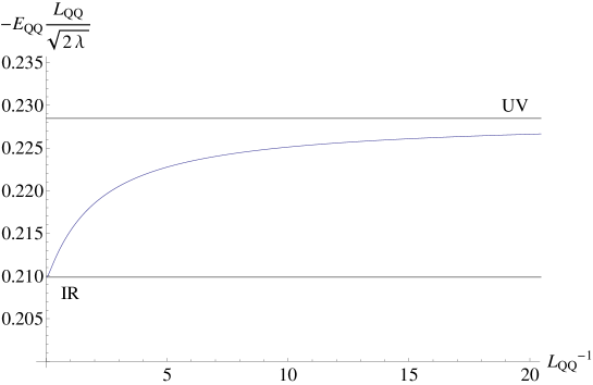
From the plot, we see how the potential interpolates between its UV value at small inter-quark separation and the IR value at very large separation, with

$$E_{\bar{Q}Q}^{UV}=-\frac{4\pi^{2}}{\Gamma\left(\frac{1}{4}\right)^{4}}\,\frac{\sqrt{2\lambda}}{L_{\bar{Q}Q}}\,\,,\qquad\qquad E_{\bar{Q}Q}^{IR}=-\sqrt{\frac{27}{32}}\frac{4\pi^{2}}{\Gamma\left(\frac{1}{4}\right)^{4}}\,\frac{\sqrt{2\lambda}}{L_{\bar{Q}Q}}\,\,,$$ (69)

where we have introduced the ’t Hooft coupling of the UV theory $\sqrt{2\lambda}=L_{UV}^{2}/\alpha^{\prime}$. At the IR and UV fixed points the potential is Coulombic as dictated by conformal invariance. The numerical factors in front of the UV and IR expressions for the potential differ by the quotient of central charges $\sqrt{c_{IR}/c_{UV}}=\sqrt{27/32}$ at the two fixed points.

The Wilson loops can also be used to probe the flows that approach the singular end-points, labelled $S_{\pm}$ and $S_{I}$ in Fig. 3. As expected, explicit computation of these physical obervables shows (see appendix B) that we should not ascribe physical meaning to these singular endpoints.

5 Anomalous dimensions of quark bilinears in the walking region

In this section we will introduce flavour fields into the gauge theory dual to the Pilch-Warner flow. The resulting theory is $SU(N)$ ${\cal N}=4$ SYM coupled to $N_{f}$ ${\cal N}=2$ hypermultiplets in the fundamental representation of the gauge group. The addition of these fields breaks the ${\cal N}=4$ supersymmetry at least down to ${\cal N}=2$. Although the hypermultiplets contain both bosonic (squark) and fermionic (quark) fields, in an abuse of language we will collectively refer to them as ‘quarks’. As usual in the ‘t Hooft limit, we consider $N\to\infty$ with $N_{f}$ fixed, so that $N_{f}\ll N$. As is well known, in this limit the quarks behave as ‘probes’ of the gluon-plus-matter-dominated dynamics. For this reason they do not break the conformal invariance of the UV and IR fixed points at leading order. In other words, their contribution to the beta-function of the theory is suppressed by $N_{f}/N$ relative to the order-$N^{2}$ contribution from the adjoints fields. Correspondingly, in the string description the quarks are described by $N_{f}$ probe D7-branes in the Pilch-Warner geometry that do not backreact on the geometry at leading order. The D7-branes wrap a three-cycle in the compact part of the geometry. The choice of this three-cycle is dual to the choice of couplings between the flavour fields and the adjoint fields in the gauge theory. Depending on the orientation of this three-cycle, these couplings will preserve or break all or part of the superymmetries. Here we will focus on a supersymmetric embedding such that the maximal possible amount of supersymmetry is preserved: ${\cal N}=2$ in the UV and ${\cal N}=1$ all along the flow, including at the IR fixed point. Thus at this point we obtain the large-$N$ Leigh-Strassler SCFT coupled to supersymmetric matter.

As explained above, our goal is to compute the dimensions at the IR fixed point of a number of operators built from quark fields. For this reason, we will focus on the dynamics of the D7-branes in the geometry dual to the LS fixed point, as opposed to the geometry dual to the entire flow. For the UV fixed point, this computation was done in Aharony:1998xz ; Kruczenski:2003be . Comparing with those references we will be able to check how dimensions change due to the RG flow to the Leigh-Strassler CFT. In other words, we will be able to compute the anomalous dimensions of the operators at the IR fixed point with respect to the UV fixed point. As emphasized in Section 1, the anomalous dimensions that we will obtain will be valid for any deformation of the ${\cal N}=4$ SYM theory that ‘walks’ near the LS fixed point. For a large class of operators the anomalous dimensions turn out to be negative and, as expected from the fact that the fixed point is strongly coupled, large. As reviewed in Section 2, large negative anomalous dimensions are an essential ingredient in phenomenologically interesting theories that exhibit walking behaviour. We will not address the departure of the theory from the walking region, i.e. away from the vicinity of the IR fixed point. We will return to this issue in Section 7, where we will discuss the possibility of eventually deviating from the walking region by deforming the D7-branes embedding.

As mentioned above, since $N_{f}\ll N$ we do not need to consider the backreaction of the D7-branes on the background geometry Karch:2002sh (see Nunez:2010sf for a recent review of holographic models in the Veneziano limit, where $N_{f}/N$ is kept fixed). The operators we will discuss are bilinears in the quark fields associated to fluctuations of the D7-branes. There are two primary reasons for focussing on these excitations rather than those of the supergravity fields (which are dual to the adjoint matter). First, this sector is simpler due to the relatively smaller number of degrees of freedom on the D7-branes compared to the number of supergravity modes. In fact, we will be able to find the scaling dimensions of all operators associated to the excitation modes of one D7-brane. Second, quark fields in the form of D7-brane probes can be expected to exhibit interesting behaviour either when the background geometry is deformed (e.g. via supersymetry-breaking deformations) or when the embedding itself is deformed away from the supersymmetric one. In such a stituation, it is possible for the D7-branes to bend and display chiral symmetry breaking as shown in Babington:2003vm ; Kruczenski:2003uq and subsequent papers. Therefore, set-ups with D7-branes can be interesting for modelling walking theories as we will discuss further in Section 7.

From now on we will focus on D7-branes sitting at $\theta=0$. It can be shown via a kappa-symmetry analysis that these branes are supersymmetric — the Killing spinors of the solution are given in Pilch:2004yg . At $\theta=0$, the probe branes wrap the squashed three-sphere with metric $e_{2}^{2}+e_{3}^{2}+e_{4}^{2}$ and $SU(2)\times U(1)$ isometry. From these symmetry considerations it is clear that the flavour D7-branes have the effect of introducing superpotential interactions between $2N_{f}$ fundamental chiral multiplets $(Q^{i},\tilde{Q}_{i})$ of the form

$$W=W_{{\cal N}=4}+\frac{1}{g^{2}_{\textrm{\tiny YM}}}\,\left[m_{3}{\rm Tr}\Phi_{3}^{2}+\sum_{i=1}^{N_{f}}Q^{i}\Phi_{3}\tilde{Q}_{i}\right]\,.$$ (70)

In order to avoid confusion, below we will denote as $q^{i}$ the fermionic component fields of the chiral superfields $Q^{i}$. The matter content and the couplings follow from ${\cal N}=2$ supersymmetry in the UV. Upon integrating out $\Phi_{3}$ we obtain a quartic superpotential that includes terms of the schematic form, $Q\tilde{Q}\,Q\tilde{Q}$. It follows that, at the Leigh-Strassler IR fixed point, we can use the non-anomalous (at large $N$) $U(1)_{R}$ to assign R-charges to the fundamental scalars (the squarks) $R[Q]=R[\tilde{Q}]=1/2$. Eqn. (6) then implies that all the quartic terms in the superpotential have dimension 3 and are therefore marginal.

5.1 Probe D7-brane dynamics

In the rest of this section we will analyze linear oscillations of a single D7-brane around the $\theta=0$ solution in the geometry dual to the LS FP, and compute the dimensions of the associated operators. At leading order in $N$, the generalization to multiple overlapping D7-branes is straightforward Kruczenski:2003uq .

The worldvolume action for the bosonic degrees of freedom of a probe D7-brane is given by the sum of Dirac-Born-Infeld (DBI) and Wess-Zumino (WZ) terms:

$$S_{D7}=-T_{7}\left(\int d^{8}x\,e^{-\phi}\sqrt{-{\rm det}(P[g]+{\cal F})}+\int P[C]\ e^{-{\cal F}}\right)$$ (71)

where $P[\ldots]$ refers to the pull-back onto the brane. From the last term of the action, one only selects the contributions from 8-forms, namely

$$\int P[C]\ e^{-{\cal F}}\equiv\int\left[P[C_{8}]-P[C_{6}]\wedge{\cal F}+\frac{1}{2}P[C_{4}]\wedge{\cal F}\wedge{\cal F}+\cdots\right]\,.$$ (72)

The two-form ${\cal F}$ is defined as:

$${\cal F}=P[B_{2}]+2\pi\alpha^{\prime}F\,,$$ (73)

where $F$ is the Abelian field strength of the worldvolume gauge field. The definition of the pull-back of the metric is:

$$P[g]_{MN}=\partial_{M}X^{A}\partial_{N}X^{B}g_{AB}\,,$$ (74)

where $M,N=1,\dots 8$ are worldvolume indices on the D7-brane, while $A,B=1,\dots,10$ are space-time indices, and the $X^{A}$ are space-time coordinates. The pull-backs of the forms are defined in a similar fashion.

As mentioned above, we want to analyze oscillations around a classical solution given by $\theta=0$, with vanishing worldvolume gauge field. A technical issue is that around $\theta=0$, the $\theta,\varphi$ coordinate system is singular. We make the following change of coordinates to a Cartesian-like system, which is well-defined in the neighbourhood of $\theta=0$:

$$z_{1}=\theta\sin\varphi\,\,,\qquad\qquad z_{2}=\theta\cos\varphi\,.$$ (75)

Since we only need to keep terms in the action which are quadratic in the fluctuations, we expand the metric up to second order in the $z$-coordinates and $B_{2}$ and $C_{6}$ to first order in $z_{1,2}$. We also find it convenient to define

$$y=L_{IR}^{-\frac{1}{4}}\,\exp\left(\frac{r}{L_{IR}}\right)\,\,.$$ (76)

In terms of this the ten-dimensional metric (61) dual to the LS fixed point, expanded to quadratic order in $z_{i}$, reads

$$ds_{10}^{2} = (1+\frac{1}{2}z_{1}^{2}+\frac{1}{2}z_{2}^{2})\left(y^{2}dx_{1,3}^{2}+L_{IR}^{\frac{3}{2}}\,\frac{dy^{2}}{y^{2}}\right)+\frac{\sqrt{3}}{4\sqrt{2}}\Bigg{[}(1-\frac{3}{2}z_{1}^{2}-\frac{3}{2}z_{2}^{2})(\sigma_{1}^{2}+\sigma_{2}^{2})+$$ (77)

$$+ \frac{4}{3}(1-2z_{1}^{2}-2z_{2}^{2})\sigma_{3}^{2}+2dz_{1}^{2}+2dz_{2}^{2}+\frac{4}{3}(z_{2}dz_{1}-z_{1}dz_{2})\sigma_{3}\Bigg{]}\,.$$

Defining $(dx)^{4}\equiv dx_{0}\wedge dx_{1}\wedge dx_{2}\wedge dx_{3}$, to first order in $z_{i}$’s, the potentials for the form fields are

$$B_{2} = -\frac{1}{4}\left[z_{2}\sigma_{1}\wedge\sigma_{3}-z_{1}\sigma_{2}\wedge\sigma_{3}+dz_{2}\wedge\sigma_{2}+dz_{1}\wedge\sigma_{1}\right]\,\,,$$

$$C_{6} = \frac{y^{4}}{16}(dx)^{4}\wedge\left[5z_{2}\sigma_{1}\wedge\sigma_{3}-5z_{1}\sigma_{2}\wedge\sigma_{3}+3dz_{2}\wedge\sigma_{2}+3dz_{1}\wedge\sigma_{1}\right]\,\,,$$

$$C_{4} = -y^{4}(dx)^{4}\,\,.$$ (78)

Here $C_{6}$ is defined by the relation $F_{7}=-{}^{*}F_{3}=dC_{6}-C_{4}\wedge H_{3}$. Notice that $C_{2}$ does not explicitly enter the quadratic action since $C_{2}\wedge B_{2}=0$. The four-form $C_{4}$ has an extra component with legs along the angles which we have not written since it does not couple to the worldvolume of the D7-brane and does not play any role in the following. It is convenient to perform a gauge transformation and to add a total derivative to $B_{2}$, in order to define a new, simpler NS-NS potential, namely:

$$B_{2}=-\frac{1}{2}\left[z_{2}\sigma_{1}\wedge\sigma_{3}-z_{1}\sigma_{2}\wedge\sigma_{3}\right]\,\,.$$ (79)

It is now a lengthy but straightforward computation to find the quadratic action for the fluctuations. We first define the determinant of the worldvolume metric at zeroth order in the fluctuations,

$$\sqrt{-g_{0}}=\frac{3\sqrt{3}}{32}y^{3}\sqrt{\tilde{g}_{3}}\,,$$ (80)

where $\tilde{g}_{3}$ denotes the metric on the squashed $S^{3}$,

$$d\tilde{s}_{3}^{2}=\sigma_{1}^{2}+\sigma_{2}^{2}+\frac{4}{3}\sigma_{3}^{2}=d\alpha_{1}^{2}+\sin^{2}\alpha_{1}d\alpha_{2}^{2}+\frac{4}{3}(d\alpha_{3}+\cos\alpha_{1}d\alpha_{2})^{2}\,.$$ (81)

From now on we will denote the squashed three-spehere as $\tilde{S}^{3}$. The metric (81) is of the type discussed in Appendix C with $a^{2}=1$, $b^{2}=4/3$. Introducing the dreibein for the squashed sphere as:

$$\tilde{e}^{1}=\sigma^{1}\,\,,\qquad\tilde{e}^{2}=\sigma^{2}\,\,,\qquad\tilde{e}^{3}=\frac{2}{\sqrt{3}}\sigma^{3}\,\,,\qquad$$ (82)

or in components $\tilde{e}^{a}=\tilde{e}_{i}^{a}d\alpha^{i}$, and the inverse dreibein as $d\alpha^{i}=e_{a}^{i}\tilde{e}^{a}$ such that $\tilde{e}_{i}^{a}e_{a}^{j}=\delta_{i}^{j}$, we have

$$\tilde{e}=\left(\begin{array}[h]{c c c}\cos\alpha_{3}&\sin\alpha_{3}&0\\ \sin\alpha_{1}\sin\alpha_{3}&-\sin\alpha_{1}\cos\alpha_{3}&\frac{2}{\sqrt{3}}\cos\alpha_{3}\\ 0&0&\frac{2}{\sqrt{3}}\end{array}\right)\,,\quad e=\left(\begin{array}[h]{c c c}\cos\alpha_{3}&\frac{\sin\alpha_{3}}{\sin\alpha_{1}}&-\frac{\sin\alpha_{3}\cos\alpha_{1}}{\sin\alpha_{1}}\\ \sin\alpha_{3}&-\frac{\cos\alpha_{3}}{\sin\alpha_{1}}&\frac{\cos\alpha_{3}\cos\alpha_{1}}{\sin\alpha_{1}}\\ 0&0&\frac{\sqrt{3}}{2}\end{array}\right)\,.$$ (83)

Notice that $\sum_{a}e_{a}^{i}e_{a}^{j}=\tilde{g}^{ij}_{3}$, the inverse metric on the squashed three-sphere. We can now write the full quadratic worldvolume action which, after subtracting a total derivative, reads:

$$-T_{7}^{-1}S_{D7}=\int d^{8}x\sqrt{-g_{0}}\Bigg{(}-\frac{1}{4}(z_{1}^{2}+z_{2}^{2})+\frac{\sqrt{3}}{4\sqrt{2}}g^{MN}(\partial_{M}z_{1}\partial_{N}z_{1}+\partial_{M}z_{2}\partial_{N}z_{2})+$$

$$+\frac{1}{2}(z_{2}\partial_{\alpha_{3}}z_{1}-z_{1}\partial_{\alpha_{3}}z_{2})+\frac{y}{2}(z_{2}\partial_{y}z_{2}+z_{1}\partial_{y}z_{1})+$$

$$+\frac{(2\pi\alpha^{\prime})^{2}}{4}F_{MN}F^{MN}-\frac{64(2\pi\alpha^{\prime})^{2}}{3^{\frac{3}{2}}}\epsilon^{abc}e_{a}^{i}e_{b}^{j}e_{c}^{k}A_{i}\partial_{\alpha_{j}}A_{k}\Bigg{)}.\,$$ (84)

In this expression the indices $M,N=1,2\ldots 8$ label the worldvolume coordinates on the D7-brane, while $i,j,k=1,2,3$ label the angular coordinates $\alpha_{i}$ of the squashed sphere. $F$ is the abelian gauge field strength on the probe D-brane, $F_{MN}=\partial_{M}A_{N}-\partial_{N}A_{M}$. It is remarkable that fluctuations $z_{i}$ of the embedding and the gauge field $A_{M}$ do not mix at quadratic order in (84). We can now extract the spectrum of fluctuations from the equations of motion that follow from (84).

There are two kinds of fluctuations on the probe brane: excitations of the brane embedding in the target space and excitations of the worldvolume gauge field. We will analyze each of these in turn below.

5.2 Fluctuations of the embedding

We first consider the two sets of oscillations transverse to the squashed three-sphere $\tilde{S}^{3}$ wrapped by the D7-brane, including their Kaluza-Klein modes on $\tilde{S}^{3}$. These include excitations of the $\theta$ coordinate around $\theta=0$. At $\theta=0$, we parametrized the transverse fluctuations in terms of the non-singular coordinates $z_{1,2}$. In the UV, the $\theta$-mode (also called the slipping mode) is dual to a dimesion-three, quark bilinear operator of the form $q^{i}{\tilde{q}}_{i}$ (cf. eqn. (70)). At the Leigh-Strassler fixed point, the equations of motion for the $z_{1}$ and $z_{2}$ fields on the D7-brane are

$$\frac{\sqrt{3}}{4\sqrt{2}y^{2}}\partial^{\mu}\partial_{\mu}z_{1}+\frac{y^{2}}{3}\partial_{y}^{2}z_{1}+\frac{5y}{3}\partial_{y}z_{1}+\frac{5}{4}z_{1}+\nabla^{2}z_{1}+\frac{1}{2}\partial_{\alpha_{3}}z_{2}=0\,\,,$$

$$\frac{\sqrt{3}}{4\sqrt{2}y^{2}}\partial^{\mu}\partial_{\mu}z_{2}+\frac{y^{2}}{3}\partial_{y}^{2}z_{2}+\frac{5y}{3}\partial_{y}z_{2}+\frac{5}{4}z_{2}+\nabla^{2}z_{2}-\frac{1}{2}\partial_{\alpha_{3}}z_{1}=0\,\,,$$ (85)

where $\nabla^{2}$ stands for the laplacian on the $\tilde{S}^{3}$ as given in (140). Inserting the scalar harmonics on the squashed sphere (see Appendix C), we can easily decouple the equations for the two modes by writing

$$z_{1}=e^{iq\cdot x}{\cal Z}_{\pm}(y)Y^{l}_{mn}(\alpha)\,\,,\qquad z_{2}=\pm i\,z_{1}\,.$$ (86)

Here $q^{\mu}$ is the four-momentum in the spacetime directions along the boundary gauge theory. We then find

$$-q^{2}\frac{\sqrt{3}}{4\sqrt{2}y^{2}}{\cal Z}_{\pm}(y)+\frac{y^{2}}{3}\partial_{y}^{2}{\cal Z}_{\pm}(y)+\frac{5y}{3}\partial_{y}{\cal Z}_{\pm}(y)+\frac{5}{4}{\cal Z}_{\pm}(y)-(\lambda\mp\frac{n}{2}){\cal Z}_{\pm}(y)=0\,\,.$$ (87)

$\lambda$ is the eigenvalue written in (141) with $a^{2}=1$, $b^{2}=4/3$, so that

$$\lambda=l(l+1)-\frac{1}{4}n^{2}\,.$$ (88)

In order to find the dimensions of the operators dual to these oscillation modes, we follow the standard AdS/CFT rules. First we determine the form of the solution of (87) near the boundary $y\to\infty$, with the result

$${\cal Z}_{\pm}(y)\sim c_{1}\,y^{-2+\frac{1}{2}\sqrt{1+12(\lambda\mp n/2)}}+c_{2}\,y^{-2-\frac{1}{2}\sqrt{1+12(\lambda\mp n/2)}}\,.$$ (89)

From this asymptotic expansion we read off the conformal dimensions of the dual field theory operators:

$$\Delta^{z}_{\pm}=2+\frac{1}{2}\sqrt{1+12l(l+1)-3n^{2}\mp 6n}\,,\qquad l=0,\frac{1}{2},1,\ldots\,,\qquad|n|\leq l\,.$$ (90)

We see that the $l=0$ mode dual to the quark bilinear $q^{i}{\tilde{q}}_{i}$ has dimension $5/2$ at the IR fixed point. The $SU(2)$ isometry of $\tilde{S}^{3}$ is dual to the global $SU(2)$ symmetry of the Leigh-Strassler SCFT, under which the chiral multiplets $\Phi_{1}$ and $\Phi_{2}$ transform as a doublet. Therefore the $SU(2)$ quantum number $l$ specifies appropriate insertions of the components of $\Phi_{1,2}$ into the fermion bilinear yielding operators in an irreducible representation of $SU(2)$. Interestingly, for $n=\pm l$ and for $n=\pm l\mp 1$, the dimensions become rational numbers:

$$\Delta^{z}_{\pm}\big{|}_{n=\pm l}=\frac{5}{2}+\frac{3}{2}l\,\,,\qquad\Delta^{z}_{\pm}\big{|}_{n=\pm l\mp 1}=3+\frac{3}{2}l\,\,.$$ (91)

5.3 Fluctuations of the worldvolume gauge field

We now turn to operators dual to fluctuations of the worldvolume gauge field on the probe D7-brane. To study these, we will first partially fix the gauge by demanding

$$\eta^{\mu\nu}\partial_{\mu}A_{\nu}=0\,.$$ (92)

Inserting this gauge choice into the equations of motion, we obtain relatively simpler expressions. There are three distinct types of gauge field components: the radial mode $A_{y}$, components $A_{i}$ along the internal directions of the $\tilde{S}^{3}$ wrapped by the D7-brane, and the four-vector $A_{\mu}$. The only contribution to the $A_{y}$ equation of motion comes from the $F_{MN}F^{MN}$ term, and it takes the form

$$\frac{\sqrt{3}}{4\sqrt{2}y^{2}}\partial^{\mu}\partial_{\mu}A_{y}+\nabla^{2}A_{y}-\partial_{y}\left[\frac{1}{\sqrt{\tilde{g}_{3}}}\partial_{i}\left(\sqrt{\tilde{g}_{3}}\,\tilde{g}^{ij}A_{j}\right)\right]=0\,.$$ (93)

Similary, the equation of motion for $A_{\nu}$ is

$$\frac{\sqrt{3}\,}{4\sqrt{2}\,y^{2}}\partial^{\mu}\partial_{\mu}A_{\nu}+\frac{1}{3y}\partial_{y}\left(y^{3}\partial_{y}A_{\nu}\right)+\nabla^{2}A_{\nu}-\partial_{\nu}\left[\frac{1}{3y}\partial_{y}(y^{3}A_{y})+\frac{1}{\sqrt{\tilde{g}_{3}}}\partial_{i}\left(\sqrt{\tilde{g}_{3}}\,\tilde{g}^{ij}A_{j}\right)\right]=0\,.$$ (94)

Finally, the linearized equation for $A_{i}$ reads

$$\tilde{g}^{mj}\left[\frac{\sqrt{3}}{4\sqrt{2}y^{2}}\partial^{\mu}\partial_{\mu}A_{j}+\frac{1}{3y^{3}}\partial_{y}(y^{5}\partial_{y}A_{j})-\frac{1}{3y^{3}}\partial_{y}(y^{5}\partial_{j}A_{y})\right]-\frac{4}{\sqrt{3}\sqrt{\tilde{g}_{3}}}\epsilon^{mjk}\partial_{j}A_{k}+$$

$$+\frac{1}{\sqrt{\tilde{g}_{3}}}\partial_{j}\left[\sqrt{\tilde{g}_{3}}\tilde{g}^{jk}\tilde{g}^{ml}(\partial_{k}A_{l}-\partial_{l}A_{k})\right]=0\,.$$ (95)

This can be written in a simpler form after contracting with $\tilde{g}_{im}$:

$$\frac{\sqrt{3}}{4\sqrt{2}y^{2}}\partial^{\mu}\partial_{\mu}A_{i}+\frac{1}{3y^{3}}\partial_{y}(y^{5}\partial_{y}A_{i})-\frac{1}{3y^{3}}\partial_{y}(y^{5}\partial_{i}A_{y})-{\cal O}_{1}({\cal O}_{1}A_{i})-\frac{4}{\sqrt{3}}{\cal O}_{1}A_{i}=0\,\,,$$ (96)

where the differential operator ${\cal O}_{1}$ is defined in (143)

Below, we analyze the spectrum of these three kinds of gauge modes, and classify them using the notation of Kruczenski:2003be .

Type I modes

We set $A_{\mu}=A_{y}=0$ and write $A_{i}$ in terms of the vector spherical harmonics on the $\tilde{S}^{3}$ described in (146)-(149) as

$$A_{i}=h_{1}^{\pm}(y)e^{iq\cdot x}\left({\bf Y}^{\pm}\right)_{i}\,.$$ (97)

With the ansatz (97), the only non-trivial equation of motion is (96), which becomes

$$-q^{2}\frac{\sqrt{3}}{4\sqrt{2}y^{2}}h_{1}^{\pm}(y)+\frac{1}{3y^{3}}\partial_{y}(y^{5}\partial_{y}h_{1}^{\pm}(y))-v_{\pm}^{2}h_{1}^{\pm}(y)-\frac{4}{\sqrt{3}}v_{\pm}\,h_{1}^{\pm}(y)=0\,.$$ (98)

As usual, the contribution from the four-momentum (the $q^{2}$ term) is subleading near the boundary ($y\to\infty$) and therefore this term can be neglected in order to compute the near-boundary solution, which takes the form

$$h_{1}^{\pm}(y)\sim c_{1}y^{-4-\sqrt{3}v_{\pm}}+c_{2}y^{\sqrt{3}v_{\pm}}\,.$$ (99)

The resulting conformal dimensions of the dual operators are then

$$\Delta^{I}_{+}=4+\sqrt{3}v_{+}\,\,,\qquad{\rm and}\,\,\qquad\Delta^{I}_{-}=-\sqrt{3}v_{-}\,\,.$$ (100)

Substituting in the eigenvalues $v_{\pm}$ from (149) we finally find

$$\Delta^{I}_{+} = 5+\frac{1}{2}\sqrt{4+12l+12l^{2}-3n^{2}}\,,\qquad l=0,\frac{1}{2},1,\ldots\,,\qquad|n|\leq l+1\,,$$

$$\Delta^{I}_{-} = -1+\frac{1}{2}\sqrt{4+12l+12l^{2}-3n^{2}}\,,\qquad l=1,\frac{3}{2},2,\ldots\,,\qquad|n|\leq l-1\,.$$ (101)

Notice that $\Delta^{I}_{+}$ becomes rational for some particular values of $n$

$$\Delta^{I}_{+}|_{|n|=l+1}=\frac{11}{2}+\frac{3}{2}l\,\,,\qquad\Delta^{I}_{+}|_{|n|=l}=6+\frac{3}{2}l\,\,.$$ (102)

Type II modes

Next we turn to the Type II modes which are dual to vector operators in the gauge theory, with $A_{y}=A_{i}=0$ and

$$A_{\mu}=\xi_{\mu}e^{iq\cdot x}h_{2}(y)Y^{l}_{mn}\,,$$ (103)

for a constant transverse polarization vector $\xi_{\mu}$. These modes are vectors in the dual field theory, as opposed to the rest of the bosonic fluctuations, which are all scalar operators. It is then clear that the only non-trivial equation is (94), which reduces to

$$-q^{2}\frac{\sqrt{3}}{4\sqrt{2}y^{2}}h_{2}(y)+\frac{1}{3y}\partial_{y}\left(y^{3}\partial_{y}h_{2}(y)\right)-\lambda\,h_{2}(y)=0\,.$$ (104)

For large $y$, the asymptotic solutions are

$$h_{2}\sim c_{1}y^{-1-\sqrt{1+3\lambda}}+c_{2}y^{-1+\sqrt{1+3\lambda}}$$ (105)

and thus, using (88), we arrive at

$$\Delta^{II}=2+\sqrt{1+3l(l+1)-3\frac{n^{2}}{4}}\,,\qquad l=0,\frac{1}{2},1,\ldots\,,\qquad|n|\leq l\,.$$ (106)

For a fixed $l$, the dimension is minimal when $n=\pm l$ and in fact $\Delta^{II}$ becomes a rational number in these cases:

$$\Delta^{II}|_{|n|=l}=3+\frac{3}{2}l\,\,.$$ (107)

Type III modes

Finally we look at the gauge field fluctuations with $A_{\mu}=0$ and

$$A_{y}=e^{iq\cdot x}h_{3}(y)Y^{l}_{mn}\,,\qquad A_{i}=e^{iq\cdot x}\tilde{h}_{3}(y)\partial_{i}Y^{l}_{mn}\,\,\,.$$ (108)

Equation (94) fixes $\tilde{h}_{3}$ in terms of $h_{3}$ as

$$\tilde{h}_{3}=\frac{1}{3y\lambda}\partial_{y}(y^{3}h_{3})\,\,,$$ (109)

and the equation of motion for $h_{3}(y)$ follows from (93):

$$-\frac{\sqrt{3}}{4\sqrt{2}y^{2}}q^{2}h_{3}+\partial_{y}\left(\frac{1}{3y}\partial_{y}(y^{3}h_{3})\right)-\lambda\,h_{3}=0\,\,,$$ (110)

while Eqn. (96) is automatically satisfied. At large $y$, the solution is

$$h_{3}\sim c_{1}y^{-2-\sqrt{1+3\lambda}}+c_{2}y^{-2+\sqrt{1+3\lambda}}$$ (111)

and thus

$$\Delta^{III}=2+\sqrt{1+3l(l+1)-3\frac{n^{2}}{4}}\,,\qquad l=\frac{1}{2},1,\frac{3}{2},\dots\,,\qquad|n|\leq l\,.$$ (112)

We point out that the trivial mode on the sphere, $\lambda=0$, is not allowed due to the factor of $\lambda$ in the denominator of Eqn. (109). This reflects the fact that $l=0$ is excluded in Eqn. (145). Apart from the absence of the $l=0$ mode, the eigenvalues (112) coincide with those for the vectors in Eqn. (106).

5.4 A discussion on the dimensions

We now compare the spectrum of operator dimensions at the IR fixed point to the UV dimensions so that we can identify the anomalous dimensions gained along the RG flow. This is easily done by comparing with the results of Aharony:1998xz ; Kruczenski:2003be , where the dimensions of these operators at the UV fixed point (${\cal N}=4$ SYM coupled to massless ${\cal N}=2$ matter) were computed. In order to translate the results of Kruczenski:2003be to our language one must make the the replacement $l\to 2l$ for all modes, as well as a subsequent shift of $l$ by $\pm 1$ for the type I $\pm$ modes. Note also that the discrete label $n$ used in the analysis of Kruczenski:2003be is unrelated to the quantum number $n$ we are using here. The final result is

$$\Delta^{z,UV}_{\pm}=\Delta^{II,UV}=\Delta^{III,UV}=3+2l\,,\qquad\Delta^{I,UV}_{+}=6+2l\,,\qquad\Delta^{I,UV}_{-}=2l\,.$$

The main points to note are as follows. First, the conformal dimensions at the IR fixed point are irrational numbers in general. At the UV fixed point all dimensions are integer-valued because the D7-brane modes fall into short multiplets of the four-dimensional ${\cal N}=2$ superconformal algebra, and hence their scaling dimensions are completely determined by their transformation properties under the $SU(2)\times U(1)$ R-symmetry of the UV theory. In contrast, the Pilch-Warner flow and the IR SCFT are only invariant under ${\cal N}=1$ supersymmetry. For this reason, the only constraint on scaling dimensions at the IR fixed point arises from holomorphy and from the charges carried by (anti)-holomorphic/chiral operators under the IR $U(1)_{R}$ symmetry. Consequently, most of the operators corresponding to fluctuations of the D7-brane have non-trivial, irrational anomalous dimensions. In particular, all the operators which are non-holomorphic or non-chiral in the ${\cal N}=1$ sense will likely acquire irrational anomalous dimensions.

Second, simple inspection shows that all the IR operators have a smaller dimension than their UV counterparts, except for the lowest type II and type I+ modes, whose dimensions

$$\Delta^{II}|_{l=0}=3\,\,\,\,\,\,\,\,\,\mbox{and}\,\,\,\,\,\,\,\,\,\Delta^{I}_{+}|_{l=0,n=0}=6$$ (113)

remain unchanged. The former is protected because the $l=0$ harmonic of the worldvolume gauge field $A_{\mu}$ is dual to a conserved $U(1)_{B}$ current in the gauge theory, and conserved vector currents must have scaling dimension 3. Under $U(1)_{B}$, which commutes with the supersymmetry generators, the superfields $Q^{i}$ and $\tilde{Q}_{i}$ transform with charges $+1$ and $-1$ respectively. The reason why the dimension of the operator dual to the type I+ mode is not renormalized is unclear to us. All operators other than the two above appear to acquire order-unity, negative anomalous dimensions along the flow.

Third, the dimension of the lowest-lying scalars describing fluctuations of the embedding are reduced from 3 in the UV to $\Delta^{z}_{\pm}|_{l=0}=5/2$ in the IR. Among these is the ‘slipping mode’ which, as discussed previously, is dual to the quark bilinear operator $q^{i}{\tilde{q}}_{i}$ that typically develops a non-trivial expectation value when supersymmetry is broken Babington:2003vm ; Kruczenski:2003uq .

Finally, it is not entirely clear to us why some of the dimensions become rational for special choices of $n$ with fixed $l$. However, it appears that in all such cases the simplified dependence on $l$ can be accounted for by insertions of the adjoint fields $\Phi_{1,2}$ in the mesonic operators. Indeed, these fields effectively have a scaling dimension of $3/4$ at the fixed point and carry ‘spin 1/2’ under the $SU(2)$ symmetry of the theory. Thus we see that $n$ insertions of the form $Q\Phi^{n}{\tilde{Q}}$ amount to increasing $l$ by $n/2$.

6 Spectrum and a light dilaton

In this section we take a first step towards analyzing the Pilch-Warner flow away from the IR fixed point and studying possible deformations driving the theory away from the walking regime. Motivated by hard-wall approaches to confining dynamics, we cut off the Pilch-Warner geometry in the infrared by hand. Because of technical convenience, we also introduce a UV cut-off, but this could be easily removed. As a consequence of the IR cut-off the spectrum becomes discrete and gapped. Our primary goal is to carefully compute this spectrum and to specifically look for a light dilaton-like state. We focus on the supergravity spectrum. In Section 7 we offer a preliminary discussion of possible studies of D7-brane dynamics in the cut-off geometry, but we leave a detailed investigation for the future.

We consider fluctuations of the system of scalars coupled to gravity around the five-dimensional background dual to the LS flow. In the language of Section 4 these are flows that start near $F_{U}$ and evolve towards the fixed point $F_{I}$. In practice, due to finite numerical precision, the flows never actually get to $F_{I}$; they can be made to get arbitrarily close to it, but eventually they all deviate away and end at a singularity. The singularity is actually of a ‘bad’ type (see section (4.3) and Appendix B) and its supergravity description is problematic. However, this will not be an obstacle because we will cut off the geometry in the IR well above the scale where any pathological behaviour sets in.

In order to compute the spectrum we will follow the algorithm and the notation of Ref. EP . In particular, we will compute the spectrum by restricting the radial direction to be compact, $r_{1}<r<r_{2}$, with hard IR and UV cut-offs $r_{1}$ and $r_{2}$, respectively. This in turn means that we will need to add localized boundary actions at the ends of the space, $r=r_{i}$, and choose appropriate boundary conditions for the fluctuations. We will always choose $r_{1}\gg r_{0}$, where $r_{0}$ is the end-of-space where all flows passing arbitrarily close to $F_{I}$ eventually end up. We also choose $r_{1}>r_{I}$, where $r_{I}$ is the scale below which the flow drifts away from the IR fixed point towards $r_{0}$. In a completely consistent walking scenario $r_{I}$ would represent the energy scale $\Lambda_{I}$ depicted in Fig. 1. As the radial dimension is compact, the resulting spectrum will be discrete. In this way, we will study the effects of the walking region on the spectrum. Due to our choice of IR cut-off the results are completely insensitive to any singularity sitting in the deep IR.

The meaning of the two cut-offs needs to be clarified. Since the geometry is asymptotically AdS, the UV cut-off could simply be removed by taking the limit $r_{2}\rightarrow+\infty$ (after inclusion of appropriate counter-terms, along the lines of holographic renormalization HR ). We will not do so because our results are not qualitatively affected by this procedure. The role of the IR cut-off is more interesting. This could be thought of as an IR regulator on the dual field theory. The fact that we choose $r_{1}>r_{I}$ means that the theory is effectively conformal in the IR all the way down to $r_{1}$, at which point confinement abruptly takes place, as modeled by the hard wall. Of course, the theory is not conformal at all scales above $r_{1}$. There is a dynamically-generated scale $r_{\ast}$ between the two cut-offs where the transition between the UV and the IR approximately-conformal dynamics takes place. The difference $r_{\ast}-r_{1}$ can be roughly thought of as the size of the walking region.

We are interested in the dependence of physical observables on $r_{\ast}$. Indeed, although the discretization of the spectrum would survive in a complete string model in which confinement arises truly dynamically, the dependence of the spectrum on the scale $r_{1}$ is likely to change. In contrast, the distortion of the spectrum due to the $r_{\ast}$ scale, provided this is far above the confining scale, would presumably remain. In summary, we wish to understand what changes in the spectrum when we keep the IR and UV cut-offs fixed but vary the boundary conditions so that $r_{\ast}$ changes. In particular, we will see that this has a crucial effect on the lightest state of the spectrum, which we would like to identify with a pseudo-dilaton.

6.1 Gauge-invariant fluctuations and numerical results

In order to determines the spectrum of scalar particles in the gauge theory we must consider fluctuations of the five-dimensional supergravity scalars with well-defined four-momentum, $\phi^{a}(q,r)$, subject to appropriate boundary conditions at $r_{i}$. The particle masses are then the values of $M^{2}=q^{2}$ for which solutions exist. This procedure is complicated by the fact that the fluctuations of the scalars source those of the five-dimensional metric. In other words, all the fluctuations are coupled. Here we will deal with this difficulty following the formalism of BHM ; EP , to which we refer the reader for further details. The idea is to write the equations of motion for the fluctuations in terms of appropiate gauge-invariant combinations of the scalar and metric fluctuations. In terms of these new scalar fields, which we denote as $\mathfrak{a}^{a}(q,r)$ following the references above, one is left (in the scalar sector) with a system of two coupled, second-order, linear differential equations.

In our present case, the formalism is greatly simplified for the following reasons:

• The five-dimensional sigma-model metric is particularly simple: the associated connection is trivial with ${\cal G}^{a}_{\,\,bc}=0$.

• The supergravity model is endowed with a superpotential $W$ (16), and hence the equations can be written in terms of $W$ and its field derivatives.

• There are only two active scalars in the system.

We also make another simplification. In defining the boundary actions, there is some freedom as to the choice of a set of couplings, which can be thought of as effective localized mass matrices for the sigma-model scalars. In general, the spectrum depends on these matrices. Furthermore, there always exist choices of such mass terms that makes one or more of the scalar excitations exactly massless. As we are mainly interested in understanding whether a light scalar excitation is admitted by the backgrounds we are considering, we take the most conservative possible attitude, and take all of these mass terms to diverge. This choice is conservative in the sense that if we find (as we will) a light state, this would still be a light state for any other choice of the boundary masses, and hence it can be taken as a physical result as opposed to an artifact associated to specific choice of boundary conditions.

The equations we have to solve involve two scalar fields $\mathfrak{a}^{a}$ related to the fluctuations of the sigma-model scalars through

$$\mathfrak{a}^{a} \equiv \varphi^{a}+\frac{W^{a}}{4W}h\,,$$ (114)

where $h$ is the trace of the four-dimensional metric fluctuations. The field derivative $W^{a}$ is evaluated on the classical background, and is defined by

$$W^{a}=G^{ab}\frac{\partial W}{\partial\phi^{a}}=\partial_{r}\phi^{a}\,.$$ (115)

The equations can then be written as

$$\begin{split}\Bigg{[}e^{-4A}\left(\delta^{a}_{b}\partial_{r}+N^{a}_{\,\,\,\,b}\right)e^{4A}\left(\delta^{b}_{c}\partial_{r}-N^{b}_{\,\,\,\,c}\right)+\delta^{a}_{c}e^{-2A}\Box\Bigg{]}\mathfrak{a}^{c}=0\,,\end{split}$$ (116)

and the boundary conditions take the form

$$\begin{split}&\left[e^{2A}\Box^{-1}\frac{W^{c}W_{d}}{W}\right]\left(\delta^{d}_{\,\,\,\,b}\partial_{r}-N^{d}_{\,\,\,\,b}\right)\mathfrak{a}^{b}\Big{|}_{r_{i}}=\delta^{c}_{\,\,\,\,b}\mathfrak{a}^{b}\Big{|}_{r_{i}}\,,\end{split}$$ (117)

where $\Box=-K^{2}=q^{2}$ is the four-dimensional momentum and

$$N^{d}_{\,\,b} \equiv G^{dc}\partial_{c}\partial_{b}W-\frac{W^{d}W_{b}}{W}\,.$$ (118)

All the functions $N$, $W$, $W_{c}$, $A$ and $W^{c}_{\,\,\,\,b}$ are evaluated on the classical background (which is known numerically).

As anticipated, the system reduces to two coupled, second-order, linear equations in the functions $\mathfrak{a}^{a}(q,r)$, subject to two sets of boundary conditions in the IR and UV. Note that the boundary conditions have the form of generalized Neumann boundary conditions, involving both the field and its derivative. However, note that in the limit in which the boundaries approach a fixed point ($W_{a}=0$) with non-trivial AdS curvature ($W<0$), the left-hand side of these expressions vanishes, and the boundary conditions reduce effectively to Dirichlet (provided $q^{2}$ is not small).

In order to determine the spectrum we first numerically generate a set backgrounds for the five-dimensional metric and scalars that describe LS flows from $F_{U}$ to $F_{I}$ in the language of Section 4. For all these flows we choose the cut-offs to be $r_{1}=2$ and $r_{2}=28$, making sure that the singularity always appears at some $r_{0}\ll r_{1}$, but vary the boundary conditions so that $r_{\ast}$ changes from flow to flow. We define $r_{\ast}$ as the value of $r$ for which the scalar ${\chi}=(\ln 3)/4$, half-way between its asymptotic UV and IR values — see Eqs. (46) and (47). We could have equivalently fixed $r_{\ast}$ and changed the position of the cut-offs, but this is less convenient numerically. Either way, the size of the walking region changes from flow to flow. We also choose the integration constant in the warp factor so that the UV-asymptotic behavior of $A(r)$ is identical for all the flows. The functions that determine the background solution, ${\alpha}(r)$, ${\chi}(r)$, and ${A}(r)$, are shown in Fig. 5 for two different flows with $r_{\ast}\simeq 0.3$ and $r_{\ast}\simeq 14$. With the flows in hand, we study scalar fluctuations as described above and detrmine the spectrum of scalar particles for each flow using the mid-point determinant method. The results are shown in Fig. 6 and Fig. 7.

Figure 5: The functions ${\alpha}$, ${\chi}$, ${A}$ and ${A}^{\prime}$ defining the backgrounds used in the calculation of the spectrum. In blue the case $r_{\ast}\simeq 14$ and in red the case $r_{\ast}\simeq 0.3$, plotted in the range $r_{1}=2<r<r_{2}=28$ used in computing the spectrum.

Figure 6: Numerical results for the spectrum, $r_{1}=2$, $r_{2}=28$, as a function of $r_{\ast}$ (see text).

Figure 7: Numerical results for the spectrum, for $r_{1}=2$, $r_{2}=28$, as a function of $r_{\ast}$ (see text). Only the lightest state is shown, together with the semi-analytical expectation.

6.2 Interpretation of the results

In order to understand some of the features that emerge from the numerical results it is useful to consider a simplified model in which the solution is a small deviation from AdS. The details are discussed in Appendix D. Here we will just describe the salient aspects of the numerical results and refer the reader to the appendix at some specific points:

• For small values of $r_{\ast}$, the spectrum agrees with the limiting case in which the background is purely AdS, with unit curvature $L=1$. Specifically, precisely as in the RS1 case, there is a massless dilaton accompanied by a tower of equally spaced KK-modes. The reason for this is simply that we are effectively turning off the deformations of the CFT living at the UV fixed point. This can be easily understood in terms of $\alpha(r_{1})$ and $\chi(r_{1})$, which, instead of approaching their IR-asymptotic values, are simply suppressed. In addition, the background has a constant $A^{\prime}=1$. This limit is not very interesting.

• For large values of $r_{\ast}$, the heavy KK states form pairs, for accidental reasons that are explained in Appendix D. When comparing the analytical example with the numerics one should replace the UV cut-off $r_{2}$ in the example, with $r_{\ast}$.

• A cross-over behavior appears at intermediate values of $r_{\ast}$. This is not surprising because the general spectrum has to interpolate between the two spectra obtained at the two fixed points.

• The two lightest states do not show the pairing displayed by the heavy states. One of them is in fact very light for any $r_{\ast}$ and exhibits a strong dependence on $r_{\ast}$ that is most interesting for our purposes. We will comment on this in more detail below. The other state is just the lightest of the $M_{+}$ states (see Appendix D) computed in the vicinity of the IR fixed point.

• The entire spectrum is mildly suppressed at relatively larger values of $r_{\ast}$. This is not an interesting physical feature; it is an artifact of the way in which we set up the calculation. In particular, we chose all the backgrounds to asymptote to AdS with $L=1$ in the far-UV. Since in the IR (below $r_{\ast}$) the background is again AdS, but with a different curvature, fixing the IR cut-off at $r_{1}=2$ corresponds to different choices of the physical IR scale. Hence the spectra computed at different values of $r_{\ast}$ are normalized with slightly different IR scales. For the KK modes, which have mass controlled by $e^{r_{1}}$, this results in a rescaling by a factor of $e^{(1-1/L_{IR})r_{\ast}}$. For the light dilaton, the rescaling is more complicated, and we will explain it later.

Before we focus on the mass of the lightest state, we perform some semi-quantitative checks. The first heavy KK-mode should have a mass (from the approximate results in Appendix D)

$$M_{11} \simeq \frac{2.4}{L_{1}}\,\equiv\,2.4\,\,e^{r_{I}}\,\simeq\,18$$ (119)

in the case in which the background is given by the UV fixed-point. This is in agreement with what we found for small values of $r_{\ast}$. The spacing between KK-modes should be

$$\Delta M \simeq \frac{\pi}{L_{1}}\,\simeq\,23\,,$$ (120)

and hence $M_{1i}\simeq 18,41,64,87\,\cdots$, which is again in remarkable agreement with the numerical results. The second such tower starts at

$$M_{21} \simeq \frac{5\pi}{4L_{1}}\,\simeq\,29\,,$$ (121)

and yields $M_{2i}=29,52,75\,\cdots$, also in agreement with the numerical results. The two towers correspond to the fluctuations of the two scalar fields which have five-dimensional masses $L^{2}M_{\textrm{\tiny scalar}}^{2}=-3,-4$ respectively — see Eqn. (52).

One can perform analogous tests at large values of $r_{\ast}$, and again very good agreement is found with the results obtained by expanding around the IR fixed-point.

Let us now turn to the lightest state in the spectrum, which becomes exactly massless in the $r_{\ast}\rightarrow\infty$ limit. Firstly, we point out that the behavior at low values of $r_{\ast}$ is uninteresting: this parametric regime corresponds to placing the IR cut-off at a very high scale, freezing out the deformations of the CFT living at the UV fixed point. More interesting is what happens when $r_{\ast}\mathrel{\raisebox{-2.58334pt}{$\stackrel{{\scriptstyle\textstyle>}}{{\sim}}$}}3$. The fact that the mass appears to be suppressed by the $r_{\ast}$ scale signals the following interpretation. While it is undoubtedly true that the dual theory is not conformal on all scales, the emergence of the light state is due to the fact that an approximate scale invariance is present in the walking region $r<r_{\ast}$. This scale invariance is approximate as it is explicitly broken by an irrelevant coupling. The spontaneous breaking is the result of our crude attempt to replace the IR with a hard-wall cut-off. This must indeed be the case, since in this region the RG flow is approaching the IR fixed point, and it would not do so if relevant deformations were present.

We can make this statement more quantitative, explicitly using our results. Notice that, because the background was obtained numerically, it does not reach the IR fixed point exactly: both the VEV and the irrelevant coupling are present. However, the former is effectively suppressed by the fact that we are close to the fixed point (and we always choose $r_{1}$ to be far from any deep-IR singularity). In the present case, the model is near-AdS only up to $r_{\ast}$, and hence in the expression Eq. (163), we should make the replacement $r_{2}\rightarrow r_{\ast}$. In order to explain the numerical results, we also need a correction factor for every appearance of $r_{1}$ in the final mass formula. In particular, we expect the lightest mass $M$ to scale as

$$M \propto \exp\left[\left(1-\sqrt{7}+\sqrt{7}(1-1/L_{IR})\right)r_{\ast}\right]\,,$$ (122)

which is in very good agreement with the numerical results, as shown in Fig. 7. Notice that in the figure an overall constant has been chosen to match the data because we are only interested in the functional dependence on $r_{\ast}$, the only physically meaningful scale in this calculation.

6.3 Comparison with Goldberger-Wise

We close with a slight digression aimed at readers who are familiar with the Goldberger-Wise mechanism GW (GW) and recognize that the formal treatment we have followed in this section is similar to what is done in that context. The main point we want to explain is that, while there are certainly analogies with the GW mechanism at the technical level, there are also important physical differences.

The basic physical problem that the GW mechanism is designed to solve is a fine-tuning problem in the basic set-up of five-dimensional effective models in which an AdS bulk is bounded by two physical cut-offs (boundaries), such as RS1 . The presence of such boundaries, and the fact that they support physical degrees of freedom, means that the theory is not scale invariant, and hence leaves open the question of why we should be allowed to assume that the two boundaries are parametrically separated. At face value this is a perfectly valid assumption as long as no other degrees of freedom are present, but it is a fine-tuned choice if we associate the two boundaries to the scales characterizing electro-weak and gravity interactions. The GW mechanism is implemented by adding a five-dimensional scalar with a small five-dimensional mass. Effectively, this can be interpreted in terms of a quasi-marginal deformation being added to the CFT dual to the AdS bulk theory. The marginal character of the deformation means that the separation of scales can be explained dynamically in terms of the exponential of the ratio between VEVs evaluated at the two boundaries, which can be chosen to be of the same order of magnitude without fine-tuning any of the parameters in the initial action. In this sense, the RS1 model, supplemented by the GW mechanism, is a brilliant effective field theory solution to the electro-weak hierarchy problem. Interestingly, this scenario leads to the presence of a light pseudo-dilaton in the spectrum GWspectrum .

What we have done in this section is substantially different for three important reasons. Firstly, the bulk geometry is not AdS, and the dual theory is not conformal; instead the bulk describes the dual of a non-trivial flow between two different fixed points characterized by a physical, dynamically-generated scale $\Lambda_{\ast}$. Second, we do not attribute any physical meaning to the two boundaries, and hence we are not interested in fine-tuning considerations involving the choices of parameters in the boundary actions. Finally, the system of scalars we write in the bulk is not dual to a quasi-marginal deformation, but rather to relevant operators that acquire large anomalous dimensions, and a resulting RG flow containing non-trivial operator-mixing effects. In practice, the above means that we are only interested in the physical effects due to those elements of the five-dmensional supergravity sigma-model that have a fully dynamical physical origin. The presence of the two boundaries is just a technical device, and we would remove them completely from the analysis if a complete flow yielding confinement in the IR were known.

7 Discussion

In this paper we have studied various aspects of the Leigh-Strassler flow and its modifications, with a view towards constructing a holographic model of quasi-conformal dynamics (walking), within a consistent supergravity/string theory framework. We have seen that a combination of the Pilch-Warner supergravity solution and a hard-wall IR cut-off exhibits a light dilaton-like state in the spectrum. We have also seen that the flow towards the strongly interacting Leigh-Strassler CFT generates large (negative) anomalous dimensions for chiral operators and for mesonic operators built from excitations of a flavor D7-brane in the geometry. Both of these are positive results from the viewpoint of using this flow to model WTC dynamics. In particular, this encourages us to look for a complete description of the flow including the departure from the IR fixed-point region to a confining vacuum within the supergravity/string framework.

Perhaps the most important question that we would like to answer in this framework is under what general conditions will a light pseudo-dilaton persist in the spectrum. The appearance of a pseudo-dilaton is associated to spontaneous breaking of approximate conformal invariance. This means that what drives the theory away from the IR fixed point is primarily a condensate for some operator, and this must be a guiding criterion in the search for a complete description of the flow.

7.1 Towards IR completions

In the hard-wall picture, conformal invariance is spontaneously broken by the IR cut-off and the details of which field theory operators condense cannot be addressed. To actually understand this, as we have explained in Section 1, we need to study the deformation of the Pilch-Warner flow by operators that make the field theory confine in the deep IR. The operators should be those that remain relevant or marginally relevant at the IR fixed point. In principle, these include supersymmetric mass deformations, certain cubic and quartic superpotential deformations of the ${\cal N}=4$ theory, or even non-supersymmetric deformations. For the ${\cal N}=1^{*}$ mass deformation, approximate IIB string backgrounds were constructed by Polchinski and Strassler PS (for equal masses), and the dynamics of IR confinement is described by 5-brane configurations that appear in the interior of the geometry. To explore the theory with a walking regime $(m_{1}=m_{2}=m\ll m_{3})$, a further deformation of this background will be necessary (see Appendix A).

For the specific case of the ${\cal N}=1^{*}$ deformation, much can be said based on field theory considerations alone. The magnitudes of all chiral condensates can be exactly computed dorey ; doreykum ; adk ; mm as functions of the masses $m_{i}$ and the gauge coupling. For example, in the confining phase it can be shown that

$$\langle{\rm Tr}\Phi_{3}^{2}\rangle\sim{N}\,m^{2}\,E_{2}\left(\frac{i}{\lambda}\right)\,,\qquad\langle{\rm Tr}\Phi_{1,2}^{2}\rangle\sim N\,m_{3}m\,E_{2}\left(\frac{i}{\lambda}\right)\,,$$ (123)

where $\lambda\equiv{g^{2}_{\textrm{\tiny YM}}N}/{4\pi}$ is the ’t Hooft coupling and $E_{2}$ is the second Eisenstein series, a quasi-modular form. Similarly, the gluino condensate depends on the combination $Nm^{2}m_{3}\,E_{2}^{\prime}\left(\frac{i}{\lambda}\right)$. All the quantities interpolate between weak coupling and the limit of large ’t Hooft coupling, corresponding to the dual supergravity limit. At strong ’t Hooft coupling we expect that the dynamical scale of confinement (set by the gluino condensate, for example) will be $\Lambda_{0}\sim(m^{2}m_{3})^{\frac{1}{3}}$, whilst the largest condensates (after factoring out their $N$-dependence) are set by the scale $\sqrt{mm_{3}}$, which is parametrically larger in the ‘walking limit’ $m_{3}\gg m$. This fact suggests that the ${\cal N}=1^{*}$ flow near the LS fixed point will be forced to deviate by large VEVS for chiral operators, which is precisely the type of situation in which we expect an approximate dilaton-like state.

A useful first step towards the construction of a string dual picture for the deformation of the Pilch-Warner flow would be to study the dual gravity description of a flow that terminates at a point on the Coulomb branch of the IR CFT Gowdigere:2005wq . Such geometries will be sourced by continuous distributions of D3-branes in the IR, encoding the VEVs on the Coulomb branch. Importantly, the flow towards the fixed point will deviate due to VEVs alone and be cut off by the D3-brane distribution. It would be interesting to understand how to extract the Goldstone mode of spontaneously broken dilatation invariance in the IR theory, from such a SUGRA background. The corresponding analysis of the spectrum from the gravity dual viewpoint, for Coulomb branch configurations of ${\cal N}=4$ SYM was perfomed in Brandhuber:2000fr ; Bianchi:2000sm .

7.2 Deformations of D7-brane embeddings

Another direction that would be interesting to explore, to look for a light scalar, lies within the probe-brane sector we have studied in this paper. In this context we would keep the gravitational background (Pilch-Warner) unchanged while having conformal symmetry broken by the embedding of the $N_{f}$ probe D7-branes. In particular, the conformal symmetry is broken in the sector of fundamental matter while the glue theory remains conformal (which is only possible in the ’t Hooft limit $N_{f}/N\to 0$).

It would then be natural to look for situations in which the fermion bilinear $q^{i}{\tilde{q}}_{i}$ condenses, namely, the ‘slipping mode’ of the D7-brane gets a non-trivial vacuum expectation value. This is only possible if supersymmetry is broken. Starting from the ${\cal N}=4$ UV fixed point, one could imagine tilting the D7-brane embedding in such a way that the supersymmetries broken by the fundamental matter fields are incompatible with those broken by the mass deformation $m_{3}$. Put another way, neither the adjoint mass deformation nor the D7-brane alone would break all the supersymmetries on their own, but the combination of both could. This can be achieved without adding an explicit mass for the fundamental flavors and is allowed since the global symmetry of ${\cal N}=4$ theory is $SU(4)$, which is larger than the manifest $SU(3)$ that rotates the three chiral adjoints once their holomorphic structure is fixed. The classical Lagrangian will still be conformally invariant but it is plausible that the slipping mode condenses and spontaneously breaks conformal symmetry of the IR fixed point (of the probe sector).

It would also be interesting to find (possibly non-supersymmetric) D7-brane embeddings which may spontaneously break the conformal symmetry of either the UV or the IR fixed point, in analogy to what was found in Kuperstein:2008cq in a different framework. It would then be very interesting to see how these D7-branes are affected by the flow and to understand how the masses of the Goldstone bosons may be lifted. We would also like to mention that seven-branes in the walking geometry of NPP have been analysed in Anguelova:2010qh .

Appendix A Relating Pilch-Warner to ${\cal N}=1^{*}$

The gravity dual of ${\cal N}=1^{*}$ was discussed by Polchinski and Strassler in PS . It is obtained by deforming ${\cal N}=4$ SYM by masses of the adjoint multiplets $\Phi_{i}$ ($i$=1,2,3). At first order, the deformation amounts to turning on the 3-form. Using notation of PS :

$$T_{3}=m_{1}dz^{1}\wedge d\bar{z}^{2}\wedge d\bar{z}^{3}+m_{2}d\bar{z}^{1}\wedge dz^{2}\wedge d\bar{z}^{3}+m_{3}d\bar{z}^{1}\wedge d\bar{z}^{2}\wedge dz^{3}+m_{4}dz^{1}\wedge dz^{2}\wedge dz^{3}$$ (124)

where we have included $m_{4}$, namely a (supersymmetry breaking) gluino mass. $T_{3}$ is proportional to the complex 3-form. The deformation leading the IR Leigh-Strassler fixed point corresponds to taking a mass for just one of the adjoint multiplets, namely $m_{1}=m_{2}=m_{4}=0$ in (124). We can then write:

$$S_{2}|_{m_{1}=m_{2}=m_{4}=0}=m_{3}\left(\bar{z}^{1}\wedge d\bar{z}^{2}\wedge dz^{3}+\bar{z}^{2}\wedge dz^{3}\wedge d\bar{z}^{1}+z^{3}d\bar{z}^{1}\wedge d\bar{z}^{2}\right)$$ (125)

such that $dS_{2}=3T_{3}$. We now check that, near the UV fixed point, the two-form of the Pilch-Warner solution written in (38) is proportional to this quantity. Using $\alpha\approx 0$, $\tanh\chi\approx m_{3}\,e^{-r}$, $X_{1}\approx 1$, we find the behaviour of (38) in the asymptotic UV:

$$C_{2}+iB_{2}|_{PW}\approx\frac{m_{3}\,e^{-r}}{2}e^{-i\,\varphi}(\cos\theta d\theta+\frac{i}{2}\,\cos^{2}\theta\sin\theta\,\sigma_{3}-i\,\cos^{2}\theta\sin\theta d\varphi)\wedge(\sigma_{1}-i\,\sigma_{2})\,\,,$$ (126)

Making contact between (125) and (126) requires writing the complex coordinates in terms of the angles. Near the UV, we can write:

$$z_{1}=e^{r}\cos\theta\,\cos\frac{\alpha_{1}}{2}e^{\frac{i}{2}(\alpha_{3}+\alpha_{2})}\,\,,\ \ z_{2}=-e^{r}\cos\theta\,\sin\frac{\alpha_{1}}{2}e^{\frac{i}{2}(\alpha_{3}-\alpha_{2})}\,\,,\ \ z_{3}=e^{r}e^{-i\,\varphi}\sin\theta\,\,.$$ (127)

It is now straightforward to check that $S_{2}|_{m_{1}=m_{2}=m_{4}=0}\approx e^{4r}(C_{2}+iB_{2})|_{PW}$.

With the above identifications, one can try to deform the PW flow with by incorporating small masses $m_{1},m_{2}$ or $m_{4}$. It is worth mentioning that in the case of PS , the deformation of ${\cal N}=4$ SYM at first order in the $m_{i}$ only includes the 3-form — for instance, the dilaton is excited only at quadratic order. Conversely, if one deforms the Pilch-Warner flow with, say, a small $m_{1}$, the dilaton is already excited at linear order in the deformation. This happens because in $F_{3}^{2}-H_{3}^{2}$ there would be terms proportional to $m_{1}\,m_{3}$ which cannot be neglected at first order since $m_{3}$ is not small in this case.

Appendix B Singular flows

In this appendix we discuss the behaviour of the classical solutions to the BPS system in Eqs. (14) and (45), in proximity of the end-points of the flows, labelled $S_{\pm}$ and $S_{I}$ in Fig. 3. In particular, we briefly discuss the physics inferred from probing the resulting geometries with strings dual to Wilson-loop operators. The asymptotic solution near $S_{U}$ is not useful for our purposes, and hence it is omitted here.

We begin by noticing that the BPS equations admit a further truncation, by fixing $\chi=0$. In this case, one is perturbing the UV fixed point by introducing mass terms and VEVs for the scalar, but not for the fermion. The resulting equation is

$$\partial_{r}\alpha = -\frac{2}{3}e^{\alpha}\sinh 3\alpha\,,$$ (128)

which admits two possible asymptotic solutions in the IR, depending on the sign of $\alpha$. Expanding the solution with positive $\alpha$ (the $S_{+}$ point in Fig. 3), and fixing an integration constant so that the singularity appears at $r_{0}=0$, at leading order in $r$ one has

$$e^{\alpha} = \left(\frac{4r}{3}\right)^{-\frac{1}{4}}\,+\,\frac{2\sqrt{2}}{15\,3^{1/4}}r^{5/4}\,+\cdots\,,$$ (129)

$$e^{A} = r^{\frac{1}{4}}\,+\,\frac{16r^{7/4}}{15\,\sqrt{3}}\,+\cdots\,.$$ (130)

By inspection of the classical equations derived from the Nambu-Goto action with this background, we find that there is no way to take $L_{QQ}\rightarrow+\infty$, in the sense that the classical system does not admit any solution with arbitrary large separation between the quak-antiquark pair. This cannot hence be interpreted as the dual of a confining theory

The solution to (128) with negative $\alpha$ (the $S_{-}$ point in Fig. 3) yields similar results. Notice however (see again Fig. 3) that the case of negative $\alpha$ is unstable, in the sense that even a small value of $\chi$ drives the flow towards the fixed point with $\chi\rightarrow+\infty$ (the point $S_{I}$). Also, notice that there are no walking flows ending near $S_{-}$, hence we are not really interested in this type of solution.

Reinstating $\chi\neq 0$ in the equations, and choosing one integration constant so that the singularity appears at ${r_{0}}=0$, the asymptotic solution around the point $S_{I}$ can be expanded as

$$e^{2\alpha} = a_{0}r^{1/7}+{\cal O}(r^{4/7})+{\cal O}(r)\,,$$ (131)

$$e^{2\chi} = \frac{6a_{0}}{7}r^{-6/7}+{\cal O}(r^{-3/7})+{\cal O}(1)\,,$$ (132)

Fixing the second integration constant $a_{0}=7/6$ for convenience, we write:

$$e^{2A} = c_{0}r^{2/7}+{\cal O}(r^{5/7})\,,$$ (133)

We may also fix the third integration constant to $c_{0}=1$, which is irrelevant for the upcoming discussion. A careful analysis shows that $L_{QQ}$ is actually finite even when the string tip approaches the singularity ($\hat{r}_{0}\rightarrow 0$), which again means that one cannot take $L_{QQ}\rightarrow+\infty$, and hence this is not interpreted as the dual description of a confining theory. The situation is very similar to that discussed in Apreda:2003sy .

In summary, we conclude that none of the possible flows ends with a healthy behaviour that can be interpreted as a signal of confinement of the dual theory (even though $S_{I}$ might yield the best toy model in that respect), and hence a radical modification of the IR geometry is needed in this respect

Appendix C Scalar and vector harmonics in the Berger sphere

In section 5, we discussed the physics of a D7-brane living in the IR fixed point of the Pilch-Warner solution. The worldvolume of the D7 is $AdS_{5}\times\tilde{S}^{3}$, where $\tilde{S}^{3}$ is the so-called Berger sphere or squashed sphere. For the analysis of section 5, it is important to know the harmonics on $\tilde{S}^{3}$, which we discuss in this appendix. In particular, we are interested in finding the eigenvalues of the Hodge-de Rham operator for scalars and vectors. The Hodge-de Rham operator acting on a $p$-form is defined, using notation of Duff:1986hr , as $\Delta=(-1)^{p}(d*d*+*d*d)$, where $d$ is the usual exterior derivative and the star represents Hodge duality.

Let us start by writing the metric of $\tilde{S}^{3}$ in terms of two constants.

$$d\tilde{s}_{3}^{2}=a^{2}(\sigma_{1}^{2}+\sigma_{2}^{2})+b^{2}\sigma_{3}^{2}=a^{2}(d\alpha_{1}^{2}+\sin^{2}\alpha_{1}d\alpha_{2}^{2})+b^{2}(d\alpha_{3}+\cos\alpha_{1}d\alpha_{2})^{2}\,\,,$$ (134)

such that the unit round $S^{3}$ is recovered with $a^{2}=b^{2}=\frac{1}{4}$ and the metric of (81) has $a^{2}=1$, $b^{2}=\frac{4}{3}$. It is useful to introduce a coordinate $z$ defined as:

$$z=\cos\alpha_{1}$$ (135)

The ranges of the different coordinates are $z\in[-1,1]$, $\alpha_{2}\in[0,2\pi)$, $\alpha_{3}\in[0,4\pi)$. In the following, we will make use of the so-called Wigner functions or $SU(2)$ functions, which we denote as $P^{l}_{mn}(z)$, following vilenkin , where their properties are discussed at length.

$$P^{l}_{mn}(z)=\frac{(-1)^{l-n}i^{n-m}}{2^{l}}\sqrt{\frac{(l+m)!}{(l-n)!(l+n)!(l-m)!}}\times$$

$$(1+z)^{\frac{-m-n}{2}}(1-z)^{\frac{n-m}{2}}\frac{d^{l-m}}{dz^{l-m}}\left[(1-z)^{l-n}(1+z)^{l+n}\right]\,\,,$$ (136)

where the allowed values of $l,m,n$ are

$$l=0,\frac{1}{2},1,\frac{3}{2},\dots,\infty\,,\qquad\ m=-l,-l+1,\dots,l-1,l\,,\qquad\ n=-l,-l+1,\dots,l-1,l\,.$$ (137)

The $P^{l}_{mn}(z)$ are generalizations of the Legendre polynomials and associated Legendre polynomials in the sense that $P_{l}(z)=P^{l}_{00}$ and $P_{l}^{m}(z)$ is a constant number times $P^{l}_{m0}(z)$ (see vilenkin for details). They solve the following second order differential equation:

$$\left[(1-z^{2})\,\partial_{zz}-2z\,\partial_{z}-\frac{m^{2}-2mnz+n^{2}}{1-z^{2}}\right]P^{l}_{mn}(z)=-l(l+1)P^{l}_{mn}(z)$$ (138)

Scalar harmonics

The scalar harmonics of the $\tilde{S}^{3}$ together with some discussion of the geometry of the squashed sphere can be found in appendix A of Zoubos:2004qm . The Hodge-de Rham operator acting on a scalar is just minus the laplacian. The eigenfunctions are given by:

$$Y^{l}_{mn}=e^{-i\,m\,\alpha_{2}-i\,n\,\alpha_{3}}P^{l}_{mn}(z)\,\,,$$ (139)

from where, using (138) we find:

$$\Delta Y_{mn}^{l}=-\nabla^{2}Y^{l}_{mn}=-\frac{1}{\sqrt{{\rm det}[g]}}\partial_{i}\left(\sqrt{{\rm det}[g]}g^{ij}\partial_{j}Y^{l}_{mn}\right)=\lambda\,Y^{l}_{mn}$$ (140)

such that the eigenvalues are:

$$\lambda=\left(\frac{l(l+1)}{a^{2}}+\left(\frac{1}{b^{2}}-\frac{1}{a^{2}}\right)n^{2}\right)$$ (141)

Vector harmonics

We have not been able to find in the literature a discussion of vector harmonics for the Berger sphere, and we present them here. The Hodge-de Rham operator acting on a vector can be written as Duff:1986hr $\Delta f_{i}=-g^{jk}\nabla_{j}\nabla_{k}f_{i}+R_{i}^{j}f_{j}$ where $\nabla$ is the usual covariant derivative and $R_{m}^{n}$ is the Ricci tensor. It can be rewritten as

$$\Delta f_{i}=-g^{jk}\nabla_{j}\nabla_{k}f_{i}+R_{i}^{j}f_{j}={\cal O}_{1}({\cal O}_{1}f_{i})+{\cal O}_{2}f_{i}\,\,,$$ (142)

where we have introduced the differential operators:

$${\cal O}_{1}f_{i}=\frac{g_{ip}}{\sqrt{{\rm det}[g]}}\epsilon^{pjk}\partial_{j}f_{k}\,\,,\qquad{\cal O}_{2}f_{i}=-\partial_{i}\left(\frac{1}{\sqrt{{\rm det}[g]}}\partial_{k}(\sqrt{{\rm det}[g]}\,g^{kj}f_{j})\right)$$ (143)

We now look for eigenvectors of (142), namely

$$\Delta f_{i}=\lambda_{v}f_{i}$$ (144)

The simplest solution to this equation is built by taking the gradient of the scalar harmonics, namely

$$\left({\bf Y}^{l}_{mn}\right)_{i}=\partial_{i}Y^{l}_{mn}\,\,,\qquad l=\frac{1}{2},1,\dots$$ (145)

The eigenvalues are again given by (141). Notice that $l=0$ is not allowed, since $\partial_{i}Y^{0}_{00}=0$.

The rest of vector harmonics are killed by ${\cal O}_{2}$ whereas they are eigenvectors of ${\cal O}_{1}$. There are two families of such solutions which we denote by $\pm$. Let us write

$${\bf Y}^{\pm}=e^{-i\,m\,\alpha_{2}-i\,n\,\alpha_{3}}\left(Y_{1}^{\pm}dz+Y_{2}^{\pm}d\alpha_{2}+Y_{3}d\alpha_{3}\right)$$ (146)

where, explicitly:

$$Y_{3}(z) = P^{l}_{mn}(z)\,\,,$$

$$Y_{2}^{\pm}(z) = \frac{(-m\,n+b^{2}v_{\pm}^{2}z)Y_{3}(z)-b\,v_{\pm}\,(1-z^{2})Y_{3}^{\prime}(z)}{b^{2}v_{\pm}^{2}-n^{2}}\,\,,$$

$$Y_{1}^{\pm}(z) = \frac{i\,(n\,Y_{2}^{\pm}(z)-m\,Y_{3}(z))}{b\,v_{\pm}\,(1-z^{2})}$$ (147)

and the eigenvalues of the ${\cal O}_{1}$ operator

$${\cal O}_{1}{\bf Y}^{\pm}=v_{\pm}{\bf Y}^{\pm}$$ (148)

are given by:

$$v_{\pm}=\frac{b^{2}\pm\sqrt{b^{4}+4a^{4}n^{2}+4a^{2}b^{2}(l^{2}+l-n^{2})}}{2a^{2}b}$$ (149)

The $\lambda_{v}$ are found by squaring these expressions. One can check that, for the $-$ mode, when $|n|=l$, the denominator in the expression for $Y_{2}^{-}$ vanishes, and there is no regular solution. Thus, the minus modes exist only for $|n|<l$. On the other hand, there is an extra solution not included in (147), found by setting $Y_{3}=0$. It can be thought of as the $n=\pm(l+1)$ generalization of the $+$ mode described above. It reads:

$${\bf Y}^{+}|_{n=\pm(l+1)}=e^{-i\,m\,\alpha_{2}\mp i\,(l+1)\,\alpha_{3}}P^{l+1}_{m,\pm(l+1)}\left(\frac{\pm i}{1-z^{2}}dz+d\alpha_{2}\right)\,\,,$$ (150)

which satisfies ${\cal O}_{1}{\bf Y}^{+}|_{n=\pm(l+1)}=(l+1)/b\ {\bf Y}^{+}|_{n=\pm(l+1)}$. Summarizing, the spectrum of the ${\cal O}_{1}$ operator reads

$$v_{+} = \frac{b^{2}+\sqrt{b^{4}+4a^{4}n^{2}+4a^{2}b^{2}(l^{2}+l-n^{2})}}{2a^{2}b}\,,\qquad\left(|n|\leq l+1,\quad l=0,\frac{1}{2},\dots\right)$$ (151)

$$v_{-} = \frac{b^{2}-\sqrt{b^{4}+4a^{4}n^{2}+4a^{2}b^{2}(l^{2}+l-n^{2})}}{2a^{2}b}\,,\qquad\left(|n|\leq l-1,\quad l=1,\frac{3}{2}\dots\right)$$ (152)

with $m=-l,\dots,l$ in all cases. It is interesting that, for $|n|=l$ and $|n|=l+1$ the square root in $v_{+}$ can be explicitly performed and we find

$$v_{+}|_{|n|=l+1}=\frac{l+1}{b}\,\,,\qquad\qquad v_{+}|_{|n|=l}=\frac{b}{a^{2}}+\frac{l}{b}\,\,.$$ (153)

As a final note, let us remark that, using the properties of the $P^{l}_{mn}(z)$, one can check that the harmonics presented are regular on the whole sphere. The easiest way to check it is to rewrite them in terms of a dreibein of (134) and make use of the fact that the leading behaviour of the Wigner function around $z=1$ is $P^{l}_{mn}(z)\sim(1-z)^{|m-n|/2}$ — apart from a multiplicative constant — and around $z=-1$ is $P^{l}_{mn}(z)\sim(1+z)^{|m+n|/2}$.

Appendix D A simplified example: Small deviations from AdS

In order to understand the numerical results presented in this Section 6, it is useful to perform a simplified exercise. We consider the case in which we are given a fully back-reacted 5D model, wherein the sigma-model has trivial kinetic terms, and the superpotential can be approximated as a quadratic function of the scalars. We also assume that the two boundaries $r_{1}$ and $r_{2}$ are chosen in such a way that effectively the whole space between them has a geometry that is close to AdS. In practice, this means that we require the two scalar sigma-model VEVs to have small values at both boundaries (and as a consequence in the whole bulk). We apply to this situation, a slight generalization of the technique used in EP to the case of the two scalars here. We pay particular attention to the calculation of the masses of the two lightest states in the two towers corresponding to the sigma-model scalars.

We begin by writing the superpotential of the canonically normalized $X^{a}$ ($a=+,-$) scalars as

$$W = -\frac{3}{2}-\frac{1}{2}X^{T}\Delta X\,,$$ (154)

where $\Delta={\rm diag}\,\{\Delta_{+},\Delta_{-}\}$ is assumed to be diagonal without loss of generailty. The BPS equations are solved by

$$X_{+} = X_{+}(r_{2})e^{-\Delta_{+}(r-r_{2})}\,,$$ (155)

$$X_{-} = X_{-}(r_{2})e^{-\Delta_{-}(r-r_{2})}\,,$$ (156)

$$A = r-\frac{1}{6}\left(X_{+}(r_{2})^{2}e^{-2\Delta_{+}(r-r_{2})}+X_{-}(r_{2})^{2}e^{-2\Delta_{-}(r-r_{2})}\right)\,,$$ (157)

where an integration constant has been chosen so that for vanishing VEVs one recovers $A=r$.

Because of our assumptions we have that $X_{\pm}(r_{1,2})\ll 1$, which in turn implies that the equations for the fluctuations can be solved perturbatively by expanding in powers of the boundary VEVs. As explained in EP , to look for the lightest solutions one needs to solve the bulk equation (116) after setting $q^{2}=0$ and all the boundary VEVs to zero (to leading order in the small VEVs), subject to the boundary conditions Eq. (LABEL:Eq:BCWinfty) in which $W$, $A$ and $N$ are evaluated by setting the VEVs to zero (leading-order). However in $W^{c}$, one keeps the leading-order dependence on the VEVs, which will then show up in $q^{2}$ as well, ensuring that all terms in all equations are written at the same (leading) order.

The bulk equations decouple from each other in this limit, and read simply

$$\Bigg{[}\left(\partial_{r}-\Delta_{+}+4\right)\left(\partial_{r}+\Delta_{+}\right)\Bigg{]}\mathfrak{a}_{+} = 0\,,$$ (158)

$$\Bigg{[}\left(\partial_{r}-\Delta_{-}+4\right)\left(\partial_{r}+\Delta_{-}\right)\Bigg{]}\mathfrak{a}_{-} = 0\,,$$ (159)

which are solved by

$$\mathfrak{a}_{+} = c_{1}^{+}e^{-\Delta_{+}r}\,+\,c_{2}^{+}e^{-(4-\Delta_{+})r}\,,$$ (160)

$$\mathfrak{a}_{-} = c_{1}^{-}e^{-\Delta_{-}r}\,+\,c_{2}^{-}e^{-(4-\Delta_{-})r}\,.$$ (161)

Note that, although the superpotential seems to suggest that the scalars decouple from each other, this is not the case: the boundary terms form a coupled system. However, at this point the system reduces to a set of four algebraic equations in the variables $q^{2}$ and $c_{i}^{\pm}$, with one arbitrary overall normalization constant:

$$-\frac{2}{3}\frac{e^{2r}}{q^{2}}\left(\begin{array}[]{cc}\Delta_{+}^{2}X_{+}(r)^{2}&\Delta_{+}X_{+}(r)\Delta_{-}X_{-}(r)\cr\Delta_{+}X_{+}(r)\Delta_{-}X_{-}(r)&\Delta_{-}^{2}X_{-}(r)^{2}\end{array}\right)\left(\partial_{r}+\left(\begin{array}[]{cc}\Delta_{+}&\cr&\Delta_{-}\end{array}\right)\right)\mathfrak{a}\Bigg{|}_{r_{i}}=\frac{}{}\mathfrak{a}\Bigg{|}_{r_{i}}\,.$$

This yields

$$q^{2} = \frac{4(\Delta_{+}-2)\Delta_{+}^{2}e^{(\Delta_{-}+5)r_{1}+(\Delta_{-}+2\Delta_{+}+5)r_{2}}X_{+}(r_{2})^{2}\frac{\sinh(r_{1}-r_{2})}{\sinh((\Delta_{+}-2)(r_{1}-r_{2}))}}{3(\cosh((\Delta_{-}+\Delta_{+}+4)(r_{1}+r_{2}))+\sinh((\Delta_{-}+\Delta_{+}+4)(r_{1}+r_{2})))}+\,(+\leftrightarrow-)\,.$$

Let us apply all of this to our example. We begin by assuming that $r_{I}\ll r_{1}\ll r_{2}\ll r_{\ast}$, so that the slice of geometry is well approximated by the IR fixed-point. From (67) we have $\Delta_{\pm}=1\pm\sqrt{7}$. After some algebra we find

$$q^{2} = \frac{8(-1+\sqrt{7})e^{2(\sqrt{7}r_{1}+r_{2})}(-e^{2r_{1}}+e^{2r_{2}})X_{-}(r_{2})^{2}}{-e^{2(1+\sqrt{7})r_{1}}+e^{2(1+\sqrt{7})r_{2}}}+$$

$$+\frac{4(1+\sqrt{7})e^{-2(r_{1}+\sqrt{7}r_{1}+2r_{2})}(-e^{2r_{1}}+e^{2r_{2}})(-e^{2(3+\sqrt{7})r_{2}}+e^{2(r_{1}+\sqrt{7}r_{1}+2r_{2})})X_{+}(r_{2})^{2}}{\cosh 2(r_{1}-r_{2})]-\cosh 2\sqrt{7}(r_{1}-r_{2})}\,,$$

$$\propto e^{2(1-\sqrt{7})r_{2}}\,,$$ (163)

where in the last line we have used the fact that $r_{2}\gg r_{1}$ and the replacement $X_{+}(r_{2})=X_{+}(r_{1})e^{-(1+\sqrt{7})(r_{2}-r_{1})}$. Which is to say that for a given (small) value of the VEV of the operator of dimension $1+\sqrt{7}$ (measured in the IR) and given (small) value for the coupling of the irrelevant operator of dimension $3+\sqrt{7}$ (measured in the UV), there is a parametrically light scalar, with exponentially suppressed mass $\propto e^{(1-\sqrt{7})r_{2}}$ as a function of the UV cut-off.

The same exercise can be carried out in the other extreme case in which $r_{\ast}\ll r_{1}\ll r_{2}$, and hence the whole geometry is close to the UV fixed point, in which case $\Delta_{\pm}=3/2\pm 1/2$. In this case,

$$q^{2} = \frac{4e^{2r_{2}-2r_{1}}}{3(r_{2}-r_{1})}\Big{(}-e^{4r_{1}-2r_{2}}r_{1}X_{-}(r_{1})^{2}+e^{4r_{1}-2r_{2}}r_{2}X_{-}(r_{1})^{2}-2e^{6r_{1}-4r_{2}}X_{+}(r_{1})^{2}+$$ (164)

$$+ 2e^{-2r_{2}+4r_{1}}X_{+}(r_{1})^{2}\Big{)}\simeq\frac{4}{3}e^{2r_{1}}\left(X_{-}(r_{1})^{2}+\frac{2}{r_{2}}X_{+}(r_{1})^{2}\right)\,,$$

where again in the last expression we use the fact that $r_{2}\gg r_{1}$. Notice that in this case one of the two deformations is the insertion of a relevant operator, and hence there is no suppression due to $r_{2}$ (the UV cut-off). The other deformation is the VEV of a dimension-two operator, and hence there is a quasi-marginal double-trace deformation producing an $r_{2}$-suppressed mass proportional to $X_{+}(r_{1})$. However, the quasi-marginal nature of the latter means that the suppression is not exponential (recall that the coordinate $r$ is related to the logarithm of the physical scale in canonical units in the dual field theory). Notice also that in both examples we applied the rule (dictated by common sense) that we express the mass as a function of the VEV of the fields $X_{\pm}$, by evaluating at $r_{1}$ those that would drive the flow away from the fixed point in the IR, while evaluating at $r_{2}$ those that would drive away the flow towards the UV.

We can perform a similar exercise in order to determine the masses of the heavy states. Now we are considering states whose mass is not suppressed by the VEVs of the sigma-model scalars. Hence we need to keep the $q^{2}$-dependence in the bulk equations, while the boundary conditions become Dirichlet:

$$\Bigg{[}\left(\partial_{r}-\Delta_{+}+4\right)\left(\partial_{r}+\Delta_{+}\right)+q^{2}e^{-2r}\Bigg{]}\mathfrak{a}_{+} = 0\,,$$ (165)

$$\Bigg{[}\left(\partial_{r}-\Delta_{-}+4\right)\left(\partial_{r}+\Delta_{-}\right)+q^{2}e^{-2r}\Bigg{]}\mathfrak{a}_{-} = 0\,,$$ (166)

$$\mathfrak{a}\Bigg{|}_{r_{i}} = 0\,.$$ (167)

The solutions can be written in terms of Bessel functions $J$ and $Y$:

$$\mathfrak{a}_{+} = e^{-2r}\left[c_{1}^{+}J_{2-\Delta_{+}}(e^{-r}q)+c_{2}^{+}Y_{2-\Delta_{+}}(e^{-r}q)\right]\,,$$ (168)

$$\mathfrak{a}_{-} = e^{-2r}\left[c_{1}^{-}J_{2-\Delta_{-}}(e^{-r}q)+c_{2}^{-}Y_{2-\Delta_{-}}(e^{-r}q)\right]\,,$$ (169)

and therefore one can easily obtain the entire spectrum.

For the case where the theory is always close to the UV fixed point, one gets for $n=1,2,\cdots$:

$$M_{+} \simeq \pi e^{r_{1}}\left(\frac{3}{4}+n-1\right)\,,$$ (170)

$$M_{-} \simeq \pi e^{r_{1}}\left(\frac{5}{4}+n-1\right)\,.$$ (171)

For the case where the theory is always close to the IR fixed point, one gets for $n=1,2,\cdots$:

$$M_{+} \simeq \pi e^{r_{1}}\left(-\frac{\sqrt{3}}{4}+n+1\right)\,,$$ (172)

$$M_{-} \simeq \pi e^{r_{1}}\left(\frac{\sqrt{3}}{4}+n+1\right)\,,$$ (173)

which fits the numerics very well. Notice in particular that, due to the numerical coincidence $\sqrt{3}/2\sim 0.9$, the two towers appear to be almost degenerate. The exceptions to this are the first light states, where the approximation is somewhat bad, and most importantly the lightest state of the $M_{+}$ series which is not paired to any state in the $M_{-}$ tower. There is no deep symmetry reason for this.