Discrimination for Two Way Models with Insurance Application

Abstract

In this paper, we review and apply several approaches to model selection for analysis of variance models which are used in a credibility and insurance context. The reversible jump algorithm is employed for model selection, where posterior model probabilities are computed. We then apply this method to insurance data from workers’ compensation insurance schemes. The reversible jump results are compared with the Deviance Information Criterion, and are shown to be consistent.

Keywords: Reversible Jump, Loss Ratios, Bayesian Analysis, Model Selection.

1 Introduction

In this paper, we address a problem posed by  klugman1987. We consider an example using the efficient proposals reversible jump method. In this example, we consider a complex two way analysis of variance model using loss ratio. We introduce alternative models of describing the process and perform model discrimination using the reversible jump algorithm.

Throughout our discussion we consider data $R$ which are insurance loss ratios. The motivation for working with loss ratios are given by hogg1984 and klugman1987. The higher levels will reflect the group to group variations in the departure from the expected losses. This will be more stable than the group to group variations in the absolute level of losses. Also we use normal models since we want to compare classical credibility models. By assuming a linear least squares approach, as in classical approach, there is a tacit assumption of normality underlying the modelling process.

Suppose that $\hbox{\boldmath$R$}_{obs}$ are the observed loss ratios, and we seek to minimise the predicted future loss ratios $\hbox{\boldmath$R$}_{new}$. The minimum expected loss is the conditional variance of $\hbox{\boldmath$R$}_{new}$ given $\hbox{\boldmath$R$}_{obs}$ and this minimum variance occurs when the predictor is the regression of $\hbox{\boldmath$R$}_{new}$ on $\hbox{\boldmath$R$}_{obs}$ i.e. the conditional expectation $\mathbb{E}(\hbox{\boldmath$R$}_{new}|\hbox{\boldmath$R$}_{obs})$. Using this decision theoretic approach we could specify a collection of candidate models, $\mathcal{M}=\{M_{i}\}$ say, then construct a decision principle based on some collection of utility functions and select the model which minimises the expected loss. In some cases, however, the specification of a utility function is not always possible and we must seek alternative approaches. In this paper, we show how an approach based on the deviance function can be used for model selection. It is assumed that a collection of plausible models exist, and we begin by asking the questions:

1. Which model explains the data we have observed?

2. Which model best predicts future observations?

3. Which model best describes the underlying process which generated the data?

We briefly review several perspectives on model selection and the connection between them before presenting our models and results.

2 General Perspective

We consider joint modelling of the parameter vector $\hbox{\boldmath$\theta$}_{k}$ and the model $M_{k}$. As noted by rubin1995, the Bayes factor is based on the assumption that one of the models being compared is the true model. However, we cannot assume this to be generally true, and we do no make this assumption. carlin1996 discusses several methods using Markov chain methods for model assessment and selection. We analyse credibility models using some of these methods. We consider model selection using posterior model probabilities based on joint modelling over the model space and parameter space. Prediction is often the ultimate goal in credibility theory. We consider model selection using predictive ability and the overall complexity of the model. We intend to use a decision theoretic approach to prediction using utility theory. We begin by motivating a decision theoretic approach and then show how this approach can be implemented using Markov Chain Monte Carlo (MCMC) methods.

bernardo1994:smith discusses several alternative views of model comparison. They are separated into three principal classes. The first is called the $\mathcal{M}$–closed system; it assumes that one of the models is the true model generating the observed data; however, it does not specifying which model is the true model. In this case, the marginal likelihood of the data is averaged over the specified model. Thus

$$p(\hbox{\boldmath$R$})=\sum_{M_{i}\in\mathcal{M}}p(M_{i})p(\hbox{\boldmath$R$}|M_{i}).$$

In addition madigan1994 show that in posterior predictive terms if $\gamma$ is a quantity of interest, averaging over the candidate models produces better results than relying on any single model.

$$\pi(\gamma|\hbox{\boldmath$R$})=\sum_{i=1}^{K}p(\gamma|M_{i},\hbox{\boldmath$R$})\pi(M_{i}|\hbox{\boldmath$R$})$$ (1)

where $\pi(M_{k}|\hbox{\boldmath$R$})$ is the posterior probability of model $M_{k}$ given the observed data and

$$p(\gamma|M_{k},\hbox{\boldmath$R$})=\int p(\gamma|\hbox{\boldmath$R$},\hbox{\boldmath$\theta$}_{k},M_{k})\pi(\hbox{\boldmath$\theta$}_{k}|\hbox{\boldmath$R$},M_{k})d\hbox{\boldmath$\theta$}_{k}.$$ (2)

For a general review of Bayesian modelling averaging, see clyde1999, and hoeting1999. However, when the set of candidate models $\mathcal{M}$ is not exhaustive, we might not be able to average over all possible models. In that context, placing a prior distribution on $\mathcal{M}$ does not apply, and since we are interested only in predicting future unknown values, this might be more appropriate than selecting a single model.

The second alternative is the so called $\mathcal{M}$-completed view, which simply seeks to compare a set of models which are available at that time. In this case $\mathcal{M}=\{M_{i}\}$ simply constitute a range of specified models to be compared. From this perspective, assigning the probabilities $\{P(M_{i}),\,M_{i}\in\mathcal{M}\}$ does not make sense and the actual overall model specifies beliefs for $R$ of the form $p(\hbox{\boldmath$R$})=p(\hbox{\boldmath$R$}|M_{t})$. Typically, $\{M_{i}\}$ will have been proposed largely because they are attractive from the point of view of tractability of analysis or communication of results, compared with the actual belief model $M_{t}$.

The third alternative is the $\mathcal{M}$-open view. In an $\mathcal{M}$-open system it is assumed that none of the models being considered is the true model which generated the observations. In this case, our goal is to select some model or subset of models which best describe the data. For the $\mathcal{M}$-completed and $\mathcal{M}$-open views, assigning prior probabilities on the model space $\mathcal{M}$ is inappropriate since statements like $p(M_{k})=c$ do not make sense. However, in the $\mathcal{M}$-open case, there is not separate overall belief specification.

3 Decision Theoretic Approach

key1999 argue that any criteria for model comparison should depend on the decision context in which the comparison is taking place, as well as the perspective from which the models are viewed. In particular, an appropriate utility structure is required, making explicit those aspects of the performance of the model that is most important. Using a decision theoretic approach, we can assign utilities to the choice of model $M_{i}$, $u(M_{i},\gamma)$, where $\gamma$ is some unknown of interest. The general decision problem is then to choose the optimal model, $M^{*}$, by maximising expected utilities

$$\bar{u}(M^{*}|\hbox{\boldmath$R$})=\sup_{\begin{subarray}{c}M_{i}\end{subarray}}\bar{u}(M_{i}|\hbox{\boldmath$R$}),$$

where

$$\bar{u}(M_{i}|\hbox{\boldmath$R$})=\int u(M_{i},\gamma)\pi(\gamma|\hbox{\boldmath$R$})d\gamma$$

with $\pi(\gamma|\hbox{\boldmath$R$})$ representing actual beliefs about $\gamma$ after observing $R$ in Equation (1).

spiegelhalter2002 propose their deviance information criterion, $DIC$, as an alternative to Bayes’ factors. In spiegelhalter2002, the $DIC$ is developed to address how well the posterior might predict future data generated by the same mechanism that gave rise to the observed data. Our motivation is that likelihood ratio tests cannot be used when there are unobservables, and that they apply only to nested models. Also likelihood ratio based tests are inconsistent, since as the sample size tends to infinity, the probability that the full model is selected does not approach zero  [GelfandGelfand1996b].

The likelihood ratio gives too much weight to the higher dimensional model, which motivates the discussion on penalised likelihoods using penalty functions. A good penalty function should depend on both the sample size and the dimension of the parameter vector. The decision theoretic approach is general enough to include traditional model selection strategies, such as choosing the model with the highest posterior probability. For example in the $\mathcal{M}$–closed system, where we assume that $\mathcal{M}$ contains the true model, if we assume a utility function of the form

$$u(M_{i},\gamma)=\begin{cases}1&\text{if $\gamma=M_{i}$}\\ 0&\text{if $\gamma\neq M_{i}$},\end{cases}$$

then from (2)

$$p(\gamma|\hbox{\boldmath$R$},M_{k})=\begin{cases}1&\text{if $\gamma=M_{i}$}\\ 0&\text{if $\gamma\neq M_{i}$}\end{cases}$$

and

$$\pi(\gamma|\hbox{\boldmath$R$})=\begin{cases}\pi(M_{i}|\hbox{\boldmath$R$})&\text{if $\gamma=M_{i}$}\\ 0&\text{if $\gamma\neq M_{i}$}.\end{cases}$$

The expected utility is then

$$\bar{u}(M_{i}|\hbox{\boldmath$R$}) =\int u(M_{i},\gamma)\pi(\gamma|\hbox{\boldmath$R$})\,d\gamma$$

$$=\pi(M_{i}|\hbox{\boldmath$R$}).$$

Therefore, the optimal decision is to choose the model with the highest posterior probability. For the $\mathcal{M}$–completed case, bernardo1994:smith shows that the cross validation predictive density yields similar results. The connection between $DIC$ and the utility approach using cross validation predictive densities, has been studied by vehtari2002, and vehtari2002:spiegelhalter who use cross validation to estimate expected utility directly, and also the effective number of parameters. The main differences are, that cross validation can be less numerically stable than the $DIC$ and can also require more computation. However, $DIC$ can underestimate the expected deviance. For a list of specific utilities used when choosing models, see key1999.

4 Computing Posterior Model Probabilities

4.1 Reversible Jump Algorithm

We assume there is a countable collection of candidate models, indexed by $M\in\mathcal{M}=\{M_{1}$, $M_{2}$,…, $M_{k}\}$. We further assume that for each model $M_{i}$, there exists an unknown parameter vector $\hbox{\boldmath$\theta$}_{i}\in\mathbb{R}^{n_{i}}$ where $n_{i}$, the dimension of the parameter vector, can vary with $M_{i}$.

Typically, we are interested in finding which models have the greatest posterior probabilities, in addition to estimates of their parameters. Thus the unknowns in this modelling scenario will include the model index $M_{i}$, as well as the parameter vector $\hbox{\boldmath$\theta$}_{i}$. We assume that the models and corresponding parameter vectors have a joint density $\pi(M_{i},\hbox{\boldmath$\theta$}_{i})$. The reversible jump algorithm constructs a reversible Markov chain on the state space $\mathcal{M}\times\bigcup_{M_{i}\in\mathcal{M}}\mathbb{R}^{n_{i}}$ which has $\pi$ as its stationary distribution [GreenGreen1995]. In many instances, and in particular for Bayesian problems, this joint distribution is

$$\pi(M_{i},\hbox{\boldmath$\theta$}_{i})=\pi(M_{i},\hbox{\boldmath$\theta$}_{i}|\hbox{\boldmath$R$})\propto\hbox{\boldmath$L$}(\hbox{\boldmath$R$}|M_{i},\hbox{\boldmath$\theta$}_{i})\;p(M_{i},\hbox{\boldmath$\theta$}_{i}),$$

where the prior on $(M_{i},\hbox{\boldmath$\theta$}_{i})$ is often of the form

$$p(M_{i},\hbox{\boldmath$\theta$}_{i})=p(\hbox{\boldmath$\theta$}_{i}|M_{i})\;p(M_{i})$$

with $p(M_{i})$ being the density of some counting distribution.

Suppose we are at model $M_{i}$, and a move to model $M_{j}$ is proposed with probability $r_{ij}$. The corresponding move from $\hbox{\boldmath$\theta$}_{i}$ to $\hbox{\boldmath$\theta$}_{j}$ is achieved by using a deterministic transformation $h_{ij}$, such that

$$(\hbox{\boldmath$\theta$}_{j},\hbox{\boldmath$v$})=h_{ij}(\hbox{\boldmath$\theta$}_{i},\hbox{\boldmath$u$}),$$ (3)

where $u$ and $v$ are random variables introduced to ensure dimension matching necessary for reversibility. To ensure dimension matching, we must have

$$\dim(\hbox{\boldmath$\theta$}_{j})+\dim(\hbox{\boldmath$v$})=\dim(\hbox{\boldmath$\theta$}_{i})+\dim(\hbox{\boldmath$u$}).$$

For discussions about possible choices for the function $h_{ij}$, we refer the reader to green1995, and brooks2003. If we denote the ratio

$$\frac{\pi(M_{j},\hbox{\boldmath$\theta$}_{j})}{\pi(M_{i},\hbox{\boldmath$\theta$}_{i})}\frac{q(\hbox{\boldmath$v$})}{q(\hbox{\boldmath$u$})}\frac{r_{ji}}{r_{ij}}\hskip 4.26773pt\biggl{\lvert}\frac{\partial h_{ij}(\hbox{\boldmath$\theta$}_{i},\hbox{\boldmath$u$})}{\partial(\hbox{\boldmath$\theta$}_{i},\hbox{\boldmath$u$})}\biggr{\rvert}$$ (4)

by $A(\hbox{\boldmath$\theta$}_{i},\hbox{\boldmath$\theta$}_{j})$, the acceptance probability for a proposed move from model $(M_{i},\hbox{\boldmath$\theta$}_{i})$ to model $(M_{j},\hbox{\boldmath$\theta$}_{j})$ is:

$$\min\left\{1,A(\hbox{\boldmath$\theta$}_{i},\hbox{\boldmath$\theta$}_{j})\right\}$$

where $q(\hbox{\boldmath$u$})$ and $q(\hbox{\boldmath$v$})$ are the respective proposal densities for $u$ and $v$, and $\lvert\partial h_{ij}(\hbox{\boldmath$\theta$}_{i},\hbox{\boldmath$u$})/\partial(\hbox{\boldmath$\theta$}_{i},\hbox{\boldmath$u$})\rvert$ is the Jacobian of the transformation induced by $h_{ij}$. It can be shown that the algorithm constructed above is reversible [GreenGreen1995] which, again, follows from the detailed balance equation

$$\pi(M_{i},\hbox{\boldmath$\theta$}_{i})q(\hbox{\boldmath$u$})r_{ij}=\pi(M_{j},\hbox{\boldmath$\theta$}_{j})q(\hbox{\boldmath$v$})r_{ji}\hskip 2.84544pt\biggl{\lvert}\frac{\partial h_{ij}(\hbox{\boldmath$\theta$}_{i},\hbox{\boldmath$u$})}{\partial(\hbox{\boldmath$\theta$}_{i},\hbox{\boldmath$u$})}\biggr{\rvert}.$$

Detailed balance is necessary to ensure reversibility and is a sufficient condition for the existence of a unique stationary distribution. For the reverse move from model $M_{j}$ to model $M_{i}$ it is easy to see that the transformation used is $(\hbox{\boldmath$\theta$}_{i},\hbox{\boldmath$u$})=h_{ij}^{-1}(\hbox{\boldmath$\theta$}_{j},\hbox{\boldmath$v$})$, and the acceptance probability for such a move is

$$\min\left\{1,\frac{\pi(M_{i},\hbox{\boldmath$\theta$}_{i})}{\pi(M_{j},\hbox{\boldmath$\theta$}_{j})}\frac{q(\hbox{\boldmath$u$})}{q(\hbox{\boldmath$v$})}\frac{r_{ij}}{r_{ji}}\hskip 4.26773pt\biggl{\lvert}\frac{\partial h_{ij}(\hbox{\boldmath$\theta$}_{i},\hbox{\boldmath$u$})}{\partial(\hbox{\boldmath$\theta$}_{i},\hbox{\boldmath$u$})}\biggr{\rvert}^{-1}\right\}=\min\left\{1,A(\hbox{\boldmath$\theta$}_{i},\hbox{\boldmath$\theta$}_{j})^{-1}\right\}.$$

For inference regarding which model has the greater posterior probability, we can base our analysis on a realisation of the Markov chain constructed above. The marginal posterior probability of model $M_{i}$

$$\pi(M_{i}|\hbox{\boldmath$R$})=\frac{p(M_{i})f(\hbox{\boldmath$R$}|M_{i})}{\sum_{M_{j}\in\mathcal{M}}p(M_{j})f(\hbox{\boldmath$R$}|M_{j})},$$

where

$$f(\hbox{\boldmath$R$}|M_{i})=\int\hbox{\boldmath$L$}(\hbox{\boldmath$R$}|M_{i},\hbox{\boldmath$\theta$}_{i})p(\hbox{\boldmath$\theta$}_{i}|M_{i})\,d\,\hbox{\boldmath$\theta$}_{i}$$

is the marginal density of the data after integrating over the unknown parameters $\theta$. In practice, we estimate $\pi(M_{i}|\hbox{\boldmath$R$})$ by counting the number of times the Markov chain visits model $M_{i}$ in a single long run after becoming stationary.

4.2 Efficient Proposals for TD MCMC

In practice, the between–model moves can be small resulting in poor mixing of the resulting Markov chain. In this section, we discuss recent attempts at improving between–model moves by increasing the acceptance probabilities for such moves. Several authors have addressed this problem, including troughton1997, giudici1998, godsill2001, rotondi2002, and alawadhi2004. green2001:mira proposes an algorithm so that when between–model moves are first rejected, a second attempt is made. This algorithm allows for a different proposal to be generated from a new distribution, that depends on the previously rejected proposal. Methods to improve mixing of reversible jump chains have also been proposed by green2002 and brooks2003; these are extended by ehlers2002.

One strategy proposed by brooks2003, and extended to more general cases by ehlers2002, is based on making the term $A_{ij}(\hbox{\boldmath$\theta$}_{i},\hbox{\boldmath$\theta$}_{j})$ in the acceptance probability for between–model moves given in Equation (4), as close as possible to 1. The motivation is that if we make this term as close as possible to 1, then the reverse move acceptance governed by $1/A_{ij}(\hbox{\boldmath$\theta$}_{i},\hbox{\boldmath$\theta$}_{j})$ will also be maximised resulting in easier between–model moves. In general, if the move from $(M_{i},\hbox{\boldmath$\theta$}_{i})\Rightarrow(M_{j},\hbox{\boldmath$\theta$}_{j})$ involves a change in dimension, the best values of the parameters for the densities $q(\hbox{\boldmath$u$})$ and $q(\hbox{\boldmath$v$})$ in Equation (4), will generally be unknown, even if their structural forms are known.

Using some known point $(\widetilde{\hbox{\boldmath$u$}},\widetilde{\hbox{\boldmath$v$}})$, which we call the centering point, we can solve $A_{ij}(\hbox{\boldmath$\theta$}_{i},\hbox{\boldmath$\theta$}_{j})=1$ to get the parameter values for these densities. Setting $A_{ij}=1$ at some chosen centering point is called the zeroth-order method. Where more degrees of freedom are required, we can expand $A_{ij}$ as a Taylor series about $(\widetilde{\hbox{\boldmath$u$}},\widetilde{\hbox{\boldmath$v$}})$ and solve for the proposal parameters. New parameters are proposed so that the mapping function in Equation (3) is the identity function, i.e.,

$$(\hbox{\boldmath$\theta$}_{j},\hbox{\boldmath$v$})=h_{ij}(\hbox{\boldmath$\theta$}_{i},\hbox{\boldmath$u$})=(\hbox{\boldmath$u$},\hbox{\boldmath$\theta$}_{i})$$

and the acceptance ratio term $A_{ij}(\hbox{\boldmath$\theta$}_{i},\hbox{\boldmath$\theta$}_{j})$ probability in Equation (4) becomes

$$A_{ij}(\hbox{\boldmath$\theta$}_{i},\hbox{\boldmath$\theta$}_{j}) =\frac{\pi(M_{j},\hbox{\boldmath$\theta$}_{j})}{\pi(M_{i},\hbox{\boldmath$\theta$}_{i})}\frac{r_{ji}}{r_{ij}}\frac{q(\hbox{\boldmath$v$})}{q(\hbox{\boldmath$u$})}$$

$$=\frac{\pi(M_{j},\hbox{\boldmath$\theta$}_{j})}{\pi(M_{i},\hbox{\boldmath$\theta$}_{i})}\frac{r_{ji}}{r_{ij}}\frac{q(\hbox{\boldmath$\theta$}_{i})}{q(\hbox{\boldmath$\theta$}_{j})}.$$

Several authors have proposed simulation methods to construct Markov chains which can explore such state spaces. These include the product space formulation given in carlin1995, the reversible jump (RJMCMC) algorithm of green1995, the jump diffusion method of  grenander1994, and phillips1996:mcmcip and the continuous time birth-death method of stephens2000. Also for particular problems involving the size of the regression vector in regression analysis, there is the stochastic search variable selection method of george1993. practice trans–dimensional algorithms work by updating model parameters for the current model, then proposing to change models with some specified probability.

4.3 Deviance Information Criterion

The $DIC$ is based on using the residual information in $X$ conditional on $\theta$, defined up to a multiplicative constant as $-2\log L(\hbox{\boldmath$X$}|\hbox{\boldmath$\theta$})$. If we have some estimate $\widetilde{\hbox{\boldmath$\theta$}}=\widetilde{\hbox{\boldmath$\theta$}}(\hbox{\boldmath$X$})$ of the true parameter, $\hbox{\boldmath$\theta$}^{t}$, then the excess residual information is

$$d(\hbox{\boldmath$X$},\hbox{\boldmath$\theta$}^{t},\widetilde{\hbox{\boldmath$\theta$}})=-2\log\hbox{\boldmath$L$}(\hbox{\boldmath$X$}|\hbox{\boldmath$\theta$}^{t})+2\log\hbox{\boldmath$L$}(\hbox{\boldmath$X$}|\widetilde{\hbox{\boldmath$\theta$}})$$

This can be thought of as the reduction in uncertainty due to estimation or the degree of overfitting due to $\widetilde{\hbox{\boldmath$\theta$}}$ adapting to the data $X$. From a Bayesian perspective $\hbox{\boldmath$\theta$}^{t}$ may be replaced by some random variable $\hbox{\boldmath$\theta$}\in\Theta$. Then $d(\hbox{\boldmath$X$},\hbox{\boldmath$\theta$}^{t},\widetilde{\hbox{\boldmath$\theta$}})$ can be estimated by its posterior expectation with respect to $\pi(\hbox{\boldmath$\theta$}|\hbox{\boldmath$X$})$ denoted

$$p_{D}(\hbox{\boldmath$X$},\Theta,\widetilde{\hbox{\boldmath$\theta$}}) =\mathbb{E}_{\hbox{\boldmath$\theta$}|\hbox{\boldmath$X$}}d(\hbox{\boldmath$X$},\hbox{\boldmath$\theta$},\widetilde{\hbox{\boldmath$\theta$}})$$

$$=\mathbb{E}(-2\log\hbox{\boldmath$L$}(\hbox{\boldmath$X$}|\hbox{\boldmath$\theta$}))+2\log\hbox{\boldmath$L$}(\hbox{\boldmath$X$}|\widetilde{\hbox{\boldmath$\theta$}}).$$

$p_{D}$ is then proposed as the effective number of parameters with respect to a model with focus $\Theta$. Thus, if we take $h(\hbox{\boldmath$X$})$ as some fully specified standardising term that is a function of the data alone, then $p_{D}$ may be written as

$$p_{D} =\overline{D(\hbox{\boldmath$\theta$})}-D(\bar{\hbox{\boldmath$\theta$}})$$

$$=\mathbb{E}_{\hbox{\boldmath$\theta$}|\hbox{\boldmath$X$}}(D(\hbox{\boldmath$\theta$}))-D(\mathbb{E}_{\hbox{\boldmath$\theta$}|\hbox{\boldmath$X$}}(\hbox{\boldmath$\theta$}))$$

where

$$D(\hbox{\boldmath$\theta$})=-2\log\hbox{\boldmath$L$}(\hbox{\boldmath$X$}|\hbox{\boldmath$\theta$})+2\log h(\hbox{\boldmath$X$}).$$ (5)

Using Bayes’ theorem we have

$$p_{D}=\mathbb{E}_{\hbox{\boldmath$\theta$}|\hbox{\boldmath$X$}}-2\log\left(\frac{\pi(\hbox{\boldmath$\theta$}|\hbox{\boldmath$X$})}{p(\hbox{\boldmath$\theta$})}\right)+2\log\left(\frac{\pi(\widetilde{\hbox{\boldmath$\theta$}}|\hbox{\boldmath$X$})}{p(\widetilde{\hbox{\boldmath$\theta$}}}\right)$$

which can be viewed as the posterior estimate of the gain in information provided by the data about $\theta$, minus the plug–in estimate of the gain in information. Having an estimate for the effective number of parameters, $p_{D}$, the quantity

$$DIC =D(\bar{\hbox{\boldmath$\theta$}})+2p_{D}$$

$$=\overline{D(\hbox{\boldmath$\theta$})}+p_{D}$$

can then be used as a Bayesian measure of fit, which when used in models with negligible prior information will be approximately equivalent to the $DIC$ criterion.

If $D(\cdot)$ in Equation (5) is available in closed form, $p_{D}$ may easily be computed using samples from an MCMC run. This is what we propose to do to measure each models complexity and then rank the models in terms of their complexity. Even though we have defined $p_{D}$ in terms of the expectation with respect to some density, other measures such as the mode or median can be used instead.

5 Discrimination for ANOVA Type Models

Quite often, the hierarchical credibility model of jewell1975 can be formulated as an analysis of variance type model. In this paper, we use reversible jump techniques to compute posterior model probabilities and compare various analysis of variance models. The reversible jump results are also compared with the results obtained by using the $DIC$.

Hierarchical models in credibility theory have been considered by jewell1975, taylor1979, zehnwirth1982, and norberg1986. Recent reviews of linear estimation for such models has been presented by goovaerts1987 and dannenburg1996. The results in this paper also have implications for other problems such as the claims reserving run-off triangle method, which we have not considered. This formulation has already been exploited by kremer1982:scandactj and ntzoufras2002, who use MCMC to estimate claim lags.

In this paper, we address a problem posed by  klugman1987 and we consider an example using the efficient proposals reversible jump method. This example is a complex two–way analysis of variance model involving loss ratios . We introduce alternative models for describing the process which generated the data, and perform model discrimination using the reversible jump algorithm.

This paper contributes to the literature on model discrimination based on reversible jumps for reparameterised Bühlmann–Straub model, a two–way model, and the hierarchical model of jewell1975. The general question is whether there is any advantage gained by using a two–way model rather than a simple random effects model in analysing the data. Even though the one–way model is a nested sub-model of the two–way model, the resulting parameter estimates can be different under both models since they have different interpretations. In this example, we see that the the two–way model is vastly superior. In the context of the Bayesian paradigm, we are able to derive posterior model probabilities and use these to discriminate between competing models. For each algorithm, the between–model moves are augmented with within–model moves which can be used to estimated model parameters for each model.

In Section 5.2, we therefore discuss how the choice of parameterisation affects the convergence of the Markov chain algorithm for within–model simulations. The between–model moves are done using the Taylor series expansion of the between–model acceptance probabilities near to some point called the centering point. In some cases using weak non–identifiable centering does not work well. Another approach, which we employ in this example, is the conditional maximisation approach, where the centering point is selected to maximise the posterior density.

5.1 The Basic Two–Way Model

Figure 1: Centred parameterisation

Figure 2: Non-centred parameterisation

The generic hierarchical model can be described as a connected graph as shown in Figure 1. Let $\theta$ denote the collection of parameters, $Y$ represent the observed data, and $X$ can take the role of missing data or other possibilities. The algorithm for sampling from the joint distribution of $\theta$, $X$, given the observed data might proceed by alternating

1. Update $\theta$ from a Markov chain with stationary distribution $\theta|X$

2. Update X from a Markov chain with stationary distribution $X|\theta,Y$

The rate of convergence of the Gibbs sampler is directly related to the choice of parameterisation for such problems. On the other hand, we might be able to find an alternative parameterisation, $(X,\theta)\rightarrow(\tilde{X},\theta)$, of the model in Figure 1 where the new missing data is some function of the previous missing data $X$ and the parameters $\theta$, such that $\tilde{X}$ is a priori independent of $\theta$. The type of parameterisation shown in Figure 2 is called non–centred parameterisation. The corresponding algorithm for simulating from the posterior distribution of $(\tilde{X},\theta)$, is then

1. Update $\theta$ from a Markov chain with stationary distribution $\theta|\tilde{X},Y$

2. Update $\tilde{X}$ from a Markov chain with stationary distribution $\tilde{X}|\theta,Y$ .

For more general discussions, see gelfand1999 and papaspilioppoulos2003.

The general form of the two–way model considered herein is the non–centred parameterisation:

$$y_{ijt}=\mu+\alpha_{i}+\beta_{j}+\gamma_{ij}+\epsilon_{ijt}\quad i=1,\ldots,m;\,j=1,\ldots,n;\,t=1,\ldots,s,$$ (6)

in which there are $s$ replications for factors $i$ and $j$. The error terms in the observations are assumed to be normally distributed and can depend on other known values. Quite often we assume that $s=1$. The interpretation of this model is that there is some overall level common to all observations, $\mu$, and then there are treatment effects that depend on the factors $i$ and $j$, denoted $\alpha_{i}$ and $\beta_{j}$, respectively. The $\gamma_{ij}$ are the interactions between the factors and they are assumed identically equal to zero.

Bayesian analysis of one-way and two-way models and general mixed linear models are studied by scheffe1959, box1973, and smith1973. The analysis of smith1973 is based on the more general normal linear model of  lindley1972. The error term $\epsilon_{ijt}$, is assumed to be normally distributed with $\epsilon_{ijt}\sim\mathcal{N}\left(0,(\sigma E_{ijt})^{-1}\right)$, where $E_{ijt}$ is some scale factor associated with observation $y_{ijt}$. The effects $\alpha_{i}$ and $\beta_{j}$ are assumed to have prior variances $1/\tau_{\alpha}$ and $1/\tau_{\beta}$, respectively. Similar models have been analysed by nobile2000, who modelled the factor terms as mixtures of normal distributions using reversible jump methods to select the number of components in the mixture. ahn1997 uses classical methods to compare their models. For the within–model parameter updates, we use the Gibbs sampler algorithm. We briefly discuss the choice of parameterisation and how different updating schemes can affect the within model convergence properties.

Before discussing how the choice of parameterisation affects the Gibbs sampler for linear mixed models, we note that the centering discussed in this section is related to the parameterisation of the models discussed, and not to the choice of centering point discussed in relation to the efficient proposals methods. For example, let

$$\eta_{i} =\mu+\alpha_{i}$$

$$\zeta_{ij} =\eta_{i}+\beta_{j}.$$

The above stated model could be reparameterised so that

$$y_{ijt} =\zeta_{ij}+\epsilon_{ijt}$$

$$\zeta_{ij} \sim\mathcal{N}\left(\eta_{i},\tau_{1}^{-1}\right)$$

$$\eta_{i} \sim\mathcal{N}\left(\mu,\tau_{2}^{-1}\right).$$

This new $(\mu,\hbox{\boldmath$\eta$},\hbox{\boldmath$\zeta$})$ parameterisation is then called the centred parameterisation, since the $\zeta_{ij}$ are centred about the $\eta_{i}$ and the $\eta_{i}$ are also centred about $\mu$. The original $(\mu,\hbox{\boldmath$\alpha$},\hbox{\boldmath$\beta$})$ parameterisation in (6) is called the non–centred parameterisation. Partial centerings are also possible, see gilks1996:mcmcip for further discussion.

5.2 Hierarchical Centering and Gibbs Updating Schemes

gelfand1995 consider general parameterisations and a hierarchically centred parameterisation by increasing the number of levels in a Bayesian analysis. They show that, if $\tau_{\beta}\rightarrow 0$ with $\tau_{\alpha}$ and $\sigma$ fixed, then the centred parameterisation will be better. If, however, $\sigma\rightarrow 0$ with $\tau_{\alpha}$ and $\tau_{\beta}$ fixed, then the non-centred parameterisation will be better. They make no optimality claims for such centerings, and generally recommend centering the random effects with the largest posterior variance to improve convergence. Thus, in the two–way model, we would centre either the $\alpha_{i}$s or the $\beta_{j}$s, provided that their variability dominated at the data level. In problems where the variance components are unknown this would necessitate a preliminary run of the algorithm to determine the variance components.

roberts1997 show that when the target density is Gaussian a deterministic scheme is most optimal for fast convergence of the Gibbs sampling algorithm for a class of structured hierarchical models. This updating scheme is also optimal for Gaussian target densities when the components can be arranged in blocks and where there is negative partial correlation between the blocks. The model parameters in the hierarchically centred parameterisation have different interpretations than those in the non–centred implementation, so direct comparison is not possible. We, however, compare both implementations using the methods of  roberts1997, whose results extend the results of  gelfand1995. Note that with the blocked parameterisation, the $\alpha_{i}$’s are conditionally independent given $\mu$, $\beta_{j}$ and $\sigma$. Therefore blocking them together does not alter the performance of the Gibbs algorithm. Blocking does not completely overcome the problems.

Block updating of the parameters should result in smaller posterior correlations amit1991,liu1994. roberts1997 and whittaker1990 show that for the parameterisation given in Equation (6), the partial correlation between any component of one block and any component of another block, is negative. In this case a random scan Gibbs algorithm or a random permutation Gibbs sampling algorithm would be expected to perform better than the deterministic scan algorithm that we use. Where the target densities are Gaussian, amit1991 recommend the use random updating strategies. However, for unknown variance components, this is not necessarily true.

When the variance components are unknown, the posterior distribution will cease to be Gaussian. The variance components will be included in the model with their respective prior specifications. The Gibbs sampler needs to sample from the joint posterior distribution of the $\mu$, $\alpha$, and $\beta$ and the variance components. However, the conditional distribution of $\mu$, $\alpha$, and $\beta$ given the variance component will still be Gaussian. Consequently, the behaviour of the Gibbs sampler should still be guided by the above considerations.

Another reason for choosing this parameterisation is that it allows for easy implementation in reversible jump schemes. It allows us to easily construct algorithms to move between models with no parameters in common as we now show, since for the one–way model, the more efficient parameterisation depends on the ratio of variances. Thus, we choose this model only because it allows for easier moves in the reversible jump scheme. For general discussions about parameterisation and MCMC implementation in linear models, see hills1992, gilks1996:mcmcip, gelfand1995, gelfand1996, and gelfand2001. The case of generalized linear models is considered by gelfand1999.

We adopt the non–centred parameterisation for the models analysed in this paper partly because the variance components are unknown. Also the non–centred parameterisation seems more readily implemented for reversible jump algorithm, since there are usually fewer model parameters. In addition, for non–centred models, the proposal distribution can easily be computed using the efficient proposals methods.

6 Example : Workers’ Compensation Insurance

In this section we analyse a set of insurance data from a Workers’ compensation scheme, using a hierarchical random effects model. A typical workers’ compensation scheme exists to provide workers who are injured in the workplace with a guaranteed source of income, until they recover and re-enter the work-force.

6.1 The Data and Model Specification

Our model is fully parametric and can be used to describe data representing workers compensation for 25 classes of occupations across 10 U.S. States, over a period of 7 years. The losses represent frequency counts on workers’ compensation insurance on permanent partial disability and the exposures are scaled payroll totals that have been inflated to represent constant dollars. We use the first 6 years of data for parameter estimation of the model; the 7th year of data is used to test the accuracy of the predictive distribution obtained. We need to estimate the class and occupation parameters, so that we have a basis for estimating future observations. The dataset has previously been analysed by klugman1992 using numerical approximations. Our approach will be hierarchical Bayesian using Markov chain Monte Carlo integration to estimate the model parameters.

The results of klugman1992 are based on matrix analytic arguments and numerical approximations of the posterior estimates of the parameters. In particular klugman1992 uses the method of Gaussian quadrature to approximate the posterior distributions of the model parameters. We present a MCMC based analysis based on the loss ratios, defined as loss / exposure. We let

$$L_{ijt} =\text{ losses for State $i$, Occupation $j$ for year $t$ }$$

$$E_{ijt} =\text{ exposure for State $i$, Occupation $j$ for year $t$ }$$

$$i =1\ldots,10,\quad j=1,\ldots,25,\quad t=1\ldots,7.$$

and the corresponding loss-ratios by $R_{ijt}$, where $R_{ijt}=L_{ijt}/E_{ijt}$.

There is one occupation class with $E_{ijt}=0$ for all $i$ and $t$ ; we removed this value of $j$ from our analysis so that data for $24$ occupation classes are left. We begin by showing how MCMC can be used to implement the original model in  klugman1992, which is a hierarchically centred model. In our analysis, we reparameterise the model and employ a non–centred model so that each level can then be compared with the first level. Other parameterisations are possible (See, for example,  venables1999). The choice of parameterisation does not affect the result, since it is the sum, $\alpha_{i}+\beta_{j}$, that really matters.

6.2 Short Review of the Klugman Model

The model described by klugman1992, which is a special case of jewell1975, has first level given by

$$R_{ijt}|\hbox{\boldmath$\alpha$},\hbox{\boldmath$\beta$},\sigma\sim\mathcal{N}\left(\alpha_{i}+\beta_{j},(\sigma E_{ijt})^{-1}\right),\,\,\,i=1,\ldots,10;j=1,\ldots,24;t=1,\ldots,6,$$ (7)

and prior structure

$$\alpha_{i}|\mu,\tau_{\alpha}\sim\mathcal{N}\left(\tfrac{1}{2}\mu,\tau_{\alpha}^{-1}\right)\quad i=1\ldots,10,$$ (8)

$$\beta_{j}|\mu,\tau_{\beta}\sim\mathcal{N}\left(\tfrac{1}{2}\mu,\tau_{\beta}^{-1}\right)\quad j=1,\ldots,24.$$ (9)

For the hyper-parameters $\sigma$, $\tau_{\alpha}$, and $\tau_{\beta}$, we use conjugate and diffuse $\text{Gamma}\left(a,b\right)$ priors. For $\mu$, we use a diffuse Gaussian prior with mean $0$ and variance $c^{-1}$. The model is a two–way model where we have made the assumption that there is no interaction between classes and occupation. The first level (7) reflects what we think about the data; that the observations are normally distributed about some mean, which does not change with time, but depends only on the class ($i$) and occupation ($j$).

We also assume the variance of any particular observation about its mean is proportional to some measure of the exposure. This assumption is popular among insurance practitioners such as ledolter1991, klugman1992, and ramlau1982. The second level comprising Equations (8) and (9), allows for any interaction between the class and occupation parameters $\hbox{\boldmath$\alpha$}=(\alpha_{1},\ldots,\alpha_{10})^{\prime}$ and $\hbox{\boldmath$\beta$}=(\beta_{1},\ldots,\beta_{24})^{\prime}$ respectively. We assume they are independent, and normally distributed with mean equal to one-half the overall mean. There is apparently no special reason for choosing such a prior for the $\alpha_{i}$ or $\beta_{j}$ parameters, other than their sum should equal the overall mean $\mu$. For our implementation we choose $a=b=c=0.001$.

6.3 The Posterior Conditional Distributions

The joint posterior distribution of the parameters, given the data, up to a constant of proportionality, takes the form:

$$\pi(\mu,\sigma,\tau_{\alpha},\tau_{\beta},\hbox{\boldmath$\alpha$},\hbox{\boldmath$\beta$}|\mathbf{E,R})\propto\\ p(\mu)p(\tau_{\alpha})p(\tau_{\beta})p(\sigma)\prod_{i=1}^{10}p(\alpha_{i}|\mu,\tau_{\alpha})\prod_{j=1}^{24}p(\beta_{j}|\mu,\tau_{\beta})\prod_{i,j,t}f(R_{ijt}|\alpha_{i},\beta_{j},\sigma).$$ (10)

From Equation (10), we can determine the following posterior conditional distributions for implementing a Gibbs updating scheme: The posterior conditional for $\alpha_{i}$ is

$$\pi(\alpha_{i}|\mu,\hbox{\boldmath$\beta$},\tau_{\alpha},\sigma,\mathbf{E,R}) \propto p(\alpha_{i}|\mu,\tau_{\alpha})\prod_{jt}f(R_{ijt}|\alpha_{i},\beta_{j},\sigma)$$

$$\alpha_{i}|\mu,\hbox{\boldmath$\beta$},\tau_{\alpha},\sigma,\mathbf{E,R} \sim\mathcal{N}\left(\frac{\tau_{\alpha}\mu/2+\sigma\sum_{jt}E_{ijt}(R_{ijt}-\beta_{j})}{\tau_{\alpha}+\sigma\sum_{jt}E_{ijt}},\frac{1}{\tau_{\alpha}+\sigma\sum_{jt}E_{ijt}}\right).$$

The posterior conditional distribution for $$\beta_{j}$$ is

$$\pi(\beta_{j}|\mu,\hbox{\boldmath$\alpha$},\tau_{\beta},\sigma,\mathbf{E,R}) \propto p(\beta_{j}|\mu,\tau_{\beta})\prod_{it}f(R_{it}|\alpha_{i},\beta_{j},\sigma)$$

$$\beta_{j}|\mu,\hbox{\boldmath$\alpha$},\tau_{\beta},\sigma,\mathbf{E,R} \sim\mathcal{N}\left(\frac{\tau_{\beta}\mu/2+\sigma\sum_{it}E_{ijt}(R_{ijt}-\alpha_{i})}{\tau_{\beta}+\sigma\sum_{it}E_{ijt}},\frac{1}{\tau_{\beta}+\sigma\sum_{it}E_{ijt}}\right).$$

The posterior conditional for $$\mu$$ is

$$\pi(\mu|\hbox{\boldmath$\alpha$},\hbox{\boldmath$\beta$},\tau_{\alpha},\tau_{\beta},\mathbf{E,R}) \propto p(\mu)\prod_{ij}p(\alpha_{i}|\mu,\tau_{\alpha})p(\beta_{j}|\mu,\tau_{\beta})$$

$$\mu|\hbox{\boldmath$\alpha$},\hbox{\boldmath$\beta$},\tau_{\alpha},\tau_{\beta},\mathbf{E,R} \sim\mathcal{N}\left(\frac{\tau_{\alpha}/2\sum_{i}\alpha_{i}+\tau_{\beta}/2\sum_{j}\beta_{j}}{c+0.25m\tau_{\alpha}+0.25n\tau_{\beta}},\frac{1}{c+0.25m\tau_{\alpha}+0.25n\tau_{\beta}}\right).$$

The posterior conditional for $$\sigma$$ is

$$\pi(\sigma|\hbox{\boldmath$\alpha$},\hbox{\boldmath$\beta$},\mathbf{E,R}) \propto p(\sigma)\prod_{ijt}f(R_{ijt}|\alpha_{i},\beta_{j},\sigma)$$

$$\sigma|\hbox{\boldmath$\alpha$},\hbox{\boldmath$\beta$},\mathbf{E,R} \sim\text{Gamma}\left(a+\frac{mns}{2},b+\tfrac{1}{2}\sum_{ijt}E_{ijt}(R_{ijt}-\alpha_{i}-\beta_{j})^{2}\right).$$

The posterior conditional distribution for $$\tau_{\alpha}$$ is

$$\pi(\tau_{\alpha}|\mu,\tau_{\alpha},\mathbf{E,R}) \propto p(\tau_{\alpha})\prod_{i}p(\alpha_{i}|\mu,\tau_{\alpha})$$

$$\tau_{\alpha}|\mu,\tau_{\alpha},\mathbf{E,R} \sim\text{Gamma}\left(a+\frac{m}{2},b+\tfrac{1}{2}\sum_{i}(\alpha_{i}-\tfrac{1}{2}\mu)^{2}\right).$$

The posterior conditional distribution for $$\tau_{\beta}$$ is

$$\pi(\tau_{\beta}|\hbox{\boldmath$\beta$},\mu,\mathbf{E,R}) \propto p(\tau_{\beta})\prod_{j}p(\beta_{j},|\mu,\tau_{\beta})$$

$$\tau_{\beta}|\hbox{\boldmath$\beta$},\mu,\mathbf{E,R} \sim\text{Gamma}\left(a+\frac{n}{2},b+\tfrac{1}{2}\sum_{j}(\beta_{j}-\tfrac{1}{2}\mu)^{2}\right).$$

6.4 Results

Tables 1 and  2 show the posterior means of the parameters with their corresponding 95% HPD intervals. The autocorrelation plots of the parameters presented in Figure 3 and Figure 4, show that mixing is not very good since there is significant dependence even at lags greater than $30$. The posterior parameter estimates are almost identical to those obtained by klugman1992 even though mixing does not appear to be good.

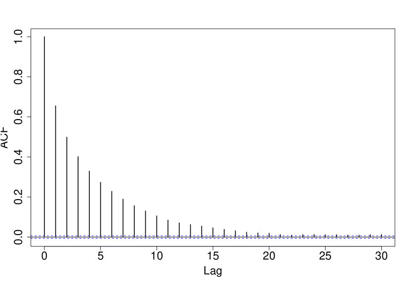
(c) $\alpha_{4}$.

(d) $\alpha_{5}$.

(e) $\alpha_{6}$.

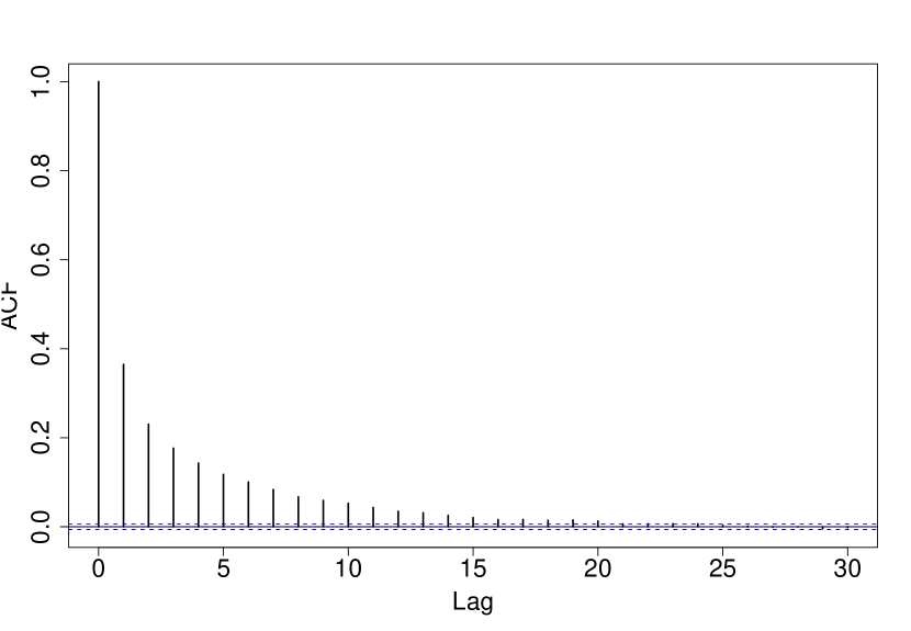
(f) $\alpha_{7}$.

(g) $\alpha_{8}$.

(h) $\alpha_{9}$.

(i) $\alpha_{10}$.

Figure 5: Autocorrelation plots for $\alpha$. The dotted lines are 95% confidence bands.

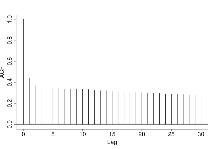
(g) $\beta_{8}$.

(h) $\beta_{9}$.

(i) $\beta_{10}$.

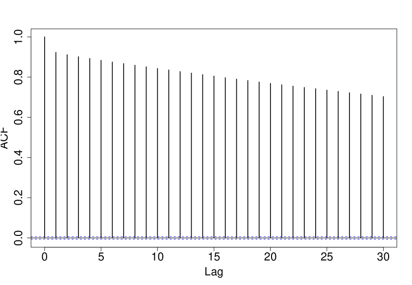
(j) $\beta_{11}$.

(k) $\beta_{12}$.

(l) $\beta_{13}$.

(m) $\beta_{14}$.

(n) $\beta_{15}$.

(o) $\beta_{16}$.

(p) $\beta_{17}$.

(q) $\beta_{18}$.

(r) $\beta_{19}$.

(s) $\beta_{20}$.

(t) $\beta_{21}$.

(u) $\beta_{22}$.

(v) $\beta_{23}$.

(w) $\beta_{24}$.

Figure 6: Autocorrelation plots for $\beta$.

In the next section, we reparameterise the model given in Section 6.2. This reparameterisation results in improved mixing for $\alpha$ and the results were marginally better for $\beta$. Figures 3 and 4 are the autocorrelation plots for the first implementation, while Figures 5 and 6 show the corresponding plots for the reparameterised implementation. The new parameterisation used is the corner point constraint, where one of the state or occupation effects is fixed at zero. Without loss of generality, we assume that $\alpha_{1}$ and $\beta_{1}$ are both identically 0. The reparameterised model is presented in Section 7.1.

(a) $\alpha_{1}$.

(b) $\alpha_{2}$.

(c) $\alpha_{3}$.

(d) $\alpha_{4}$.

(e) $\alpha_{5}$.

(f) $\alpha_{6}$.

(g) $\alpha_{7}$.

(h) $\alpha_{8}$.

(i) $\alpha_{9}$.

(j) $\alpha_{10}$.

Figure 3: Autocorrelation plots for $\alpha$.

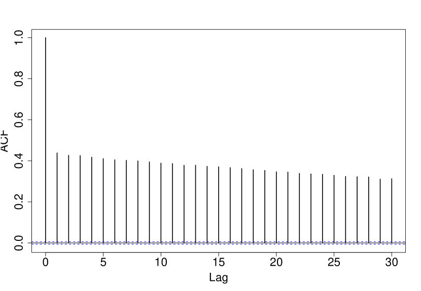
(a) $\beta_{1}$.

(b) $\beta_{2}$.

(c) $\beta_{3}$.

(d) $\beta_{4}$.

(e) $\beta_{5}$.

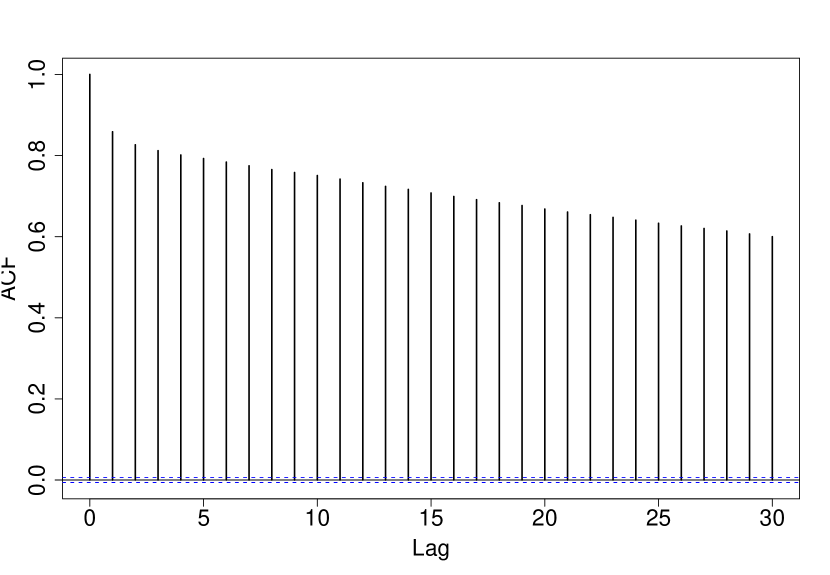
(f) $\beta_{6}$.

(g) $\beta_{7}$.

(h) $\beta_{8}$.

(i) $\beta_{9}$.

(j) $\beta_{10}$.

(k) $\beta_{11}$.

(l) $\beta_{12}$.

(m) $\beta_{13}$.

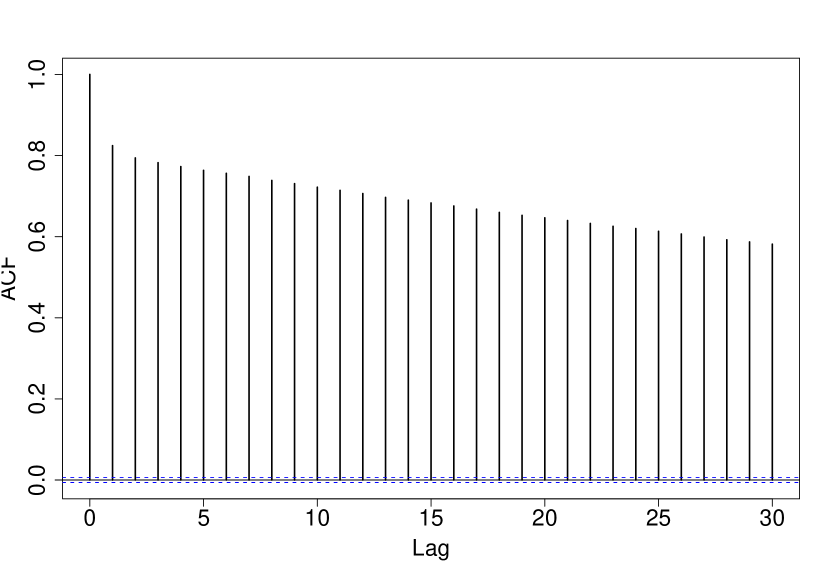
(n) $\beta_{14}$.

(o) $\beta_{15}$.

(p) $\beta_{16}$.

(q) $\beta_{17}$.

(r) $\beta_{18}$.

(s) $\beta_{19}$.

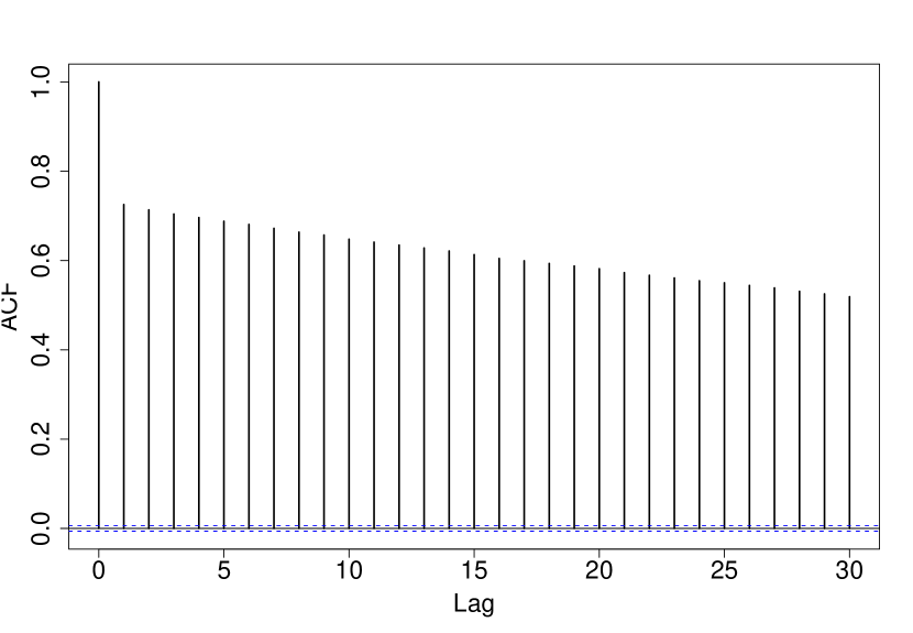
(t) $\beta_{20}$.

(u) $\beta_{21}$.

(v) $\beta_{22}$.

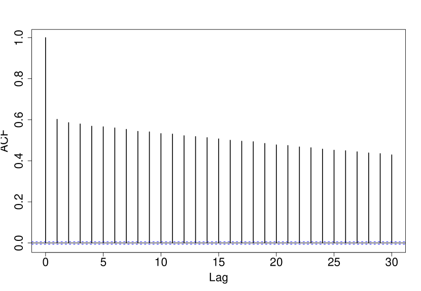
(w) $\beta_{23}$.

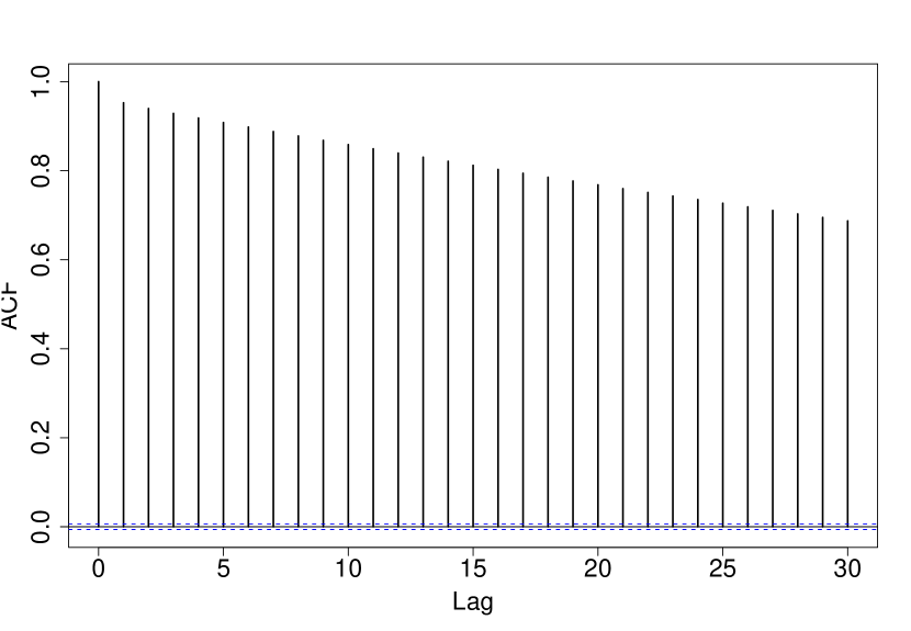
(x) $\beta_{24}$.

Figure 4: Autocorrelation plots for $\beta$.

We also investigate whether the state effects ($i$) are substantial and also whether the occupation effects ($j$) are non–trivial. For this, we employ the reversible jump algorithm. In the absence of a natural jump function, we propose to change all model parameters when moving between models. This is not strictly necessary. However, if parameter values change substantially between models, then keeping such values fixed will result in high reject rates at the accept/reject stage of the Reversible jump algorithm. We discuss the reversible jump algorithm for this example in Section 8.2.

Table 1: Estimates of the model parameters, with 95% HPD Intervals.

	mean	95% HPD Interval
$\alpha_{1}$	0.0095	(-0.0085, 0.0270)
$\alpha_{2}$	0.0492	(0.0310, 0.0676)
$\alpha_{3}$	0.0993	(0.0687, 0.1305)
$\alpha_{4}$	0.0310	(0.0134, 0.0487)
$\alpha_{5}$	0.0068	(-0.0113, 0.0246)
$\alpha_{6}$	0.0322	(0.0131, 0.0507)
$\alpha_{7}$	0.0100	(-0.0090, 0.0290)
$\alpha_{8}$	0.1109	(0.0926, 0.1291)
$\alpha_{9}$	0.0067	(-0.0131, 0.0263)
$\alpha_{10}$	0.0525	(0.0312, 0.0738)

Table 2: Estimates of the model parameters, with 95% HPD Intervals.

	mean	95% HPD Interval
$\beta_{1}$	0.0711	(0.0458, 0.0967)
$\beta_{2}$	0.0792	(0.0545, 0.1042)
$\beta_{3}$	0.0206	(0.0009, 0.0403)
$\beta_{4}$	-0.0269	(-0.0667, 0.0131)
$\beta_{5}$	0.0539	(0.0351, 0.0729)
$\beta_{6}$	0.1873	(0.1684, 0.2060)
$\beta_{7}$	0.0924	(0.0606, 0.1243)
$\beta_{8}$	0.0532	(0.0246, 0.0822)
$\beta_{9}$	0.0120	(-0.0074, 0.0317)
$\beta_{10}$	0.0360	(0.0160, 0.0561)
$\beta_{11}$	0.0206	(0.0026, 0.0387)
$\beta_{12}$	0.0308	(0.0111, 0.0503)
$\beta_{13}$	0.0392	(0.0194, 0.0592)
$\beta_{14}$	0.0515	(0.0326, 0.0708)
$\beta_{15}$	0.0816	(0.0617, 0.1017)
$\beta_{16}$	0.0306	(0.0114, 0.0503)
$\beta_{17}$	0.0222	(-0.0051, 0.0494)
$\beta_{18}$	0.0178	(-0.0162, 0.0516)
$\beta_{19}$	0.0256	(0.0074, 0.0440)
$\beta_{20}$	0.0143	(-0.0058, 0.0346)
$\beta_{21}$	0.0307	(0.0119, 0.0494)
$\beta_{22}$	0.0034	(-0.0170, 0.0237)
$\beta_{23}$	0.0357	(0.0137, 0.0578)
$\beta_{24}$	-0.0003	(-0.0178, 0.0176)

7 Reparameterisation Issues

We reparameterise the model to allow for more freedom of the first level parameters. In model  (7), both $\alpha_{i}$ and $\beta_{j}$ are restricted to have mean $\mu/2$. There is, however, no direct interpretation of the model parameters, given this parameterisation

In addition, we reparameterise the model so that each state effect and occupation effect are compared with the first level. For this, we set both $\alpha_{1}$ and $\beta_{1}$ equal to zero. This is the well known corner point constraint [Venables and RipleyVenables and Ripley1999, Section 6.2]. The reparameterised model is

$$R_{ijt}|\mu,\hbox{\boldmath$\alpha$},\hbox{\boldmath$\beta$},\sigma\sim\mathcal{N}\left(\mu+\alpha_{i}+\beta_{j},(\sigma E_{ijt})^{-1}\right),\quad\alpha_{1}=0,\,\,\beta_{1}=0.$$ (11)

We use multivariate normal priors for $\hbox{\boldmath$\alpha$}=(\alpha_{2},\ldots,\alpha_{m})^{\prime}$ and $\hbox{\boldmath$\beta$}=(\beta_{2},\ldots,\beta_{n})^{\prime}$. The derivation of the posterior conditional distributions are given in the next section.

The reparameterisation does not affect the final interpretation of the model. It could, however, affect the convergence rate of the Gibbs sampler. Problems such as these are considered by  papaspilioppoulos2003 who show that the centered parameterisation is not uniformly superior to the non–centered parameterisation, and indeed that a partially centered parameterisation might give the fastest convergence rate of the Gibbs sampler. We also note that the autocorrelations have decreased because of the parameterisations chosen. Generally the autocorrelation for hierarchical models depends on the parameterisation chosen. See for example gilks1996:mcmcip, gelfand1995, and gelfand1996.

7.1 Using Non–Centred Block Updates

Let $\hbox{\boldmath$\alpha$}=(\alpha_{2},\ldots,\alpha_{m})^{\prime}$, $\hbox{\boldmath$\beta$}=(\beta_{2},\ldots,\beta_{n})^{\prime}$ and, as before, let $\hbox{\boldmath$R$}=\{R_{ijt}\}$ denote the loss ratios. The first level is described as

$$R_{ijt}\sim\mathcal{N}\left(\mu+\alpha_{i}+\beta_{j},(\sigma E_{ijt})^{-1}\right),\quad\alpha_{1}=0,\,\,\,\beta_{1}=0.$$

Given the first above, we choose the following prior distributions for the model parameters

$$\mu\sim\mathcal{N}\left(0,\tau_{\mu}^{-1}\right),\;\hbox{\boldmath$\alpha$}\sim\mathcal{N}\left(\hbox{\boldmath$0$},\tau_{\alpha}^{-1}\hbox{\boldmath$I$}\right),\;\hbox{\boldmath$\beta$}\sim\mathcal{N}\left(\hbox{\boldmath$0$},\tau_{\beta}^{-1}\hbox{\boldmath$I$}\right),\text{ and }\sigma\sim\text{Gamma}\left(a,b\right),$$

where $\tau_{\mu}=\tau_{\alpha}=\tau_{\beta}=0.001$, and $a=b=0.001$, so that these prior distributions are vague and flat. The law of $(\hbox{\boldmath$\alpha$},\hbox{\boldmath$\beta$},\mu,\sigma)$, given the data is

$$\pi(\mu,\hbox{\boldmath$\alpha$},\hbox{\boldmath$\beta$},\sigma|\hbox{\boldmath$R$})\propto p(\sigma)p(\mu)p(\hbox{\boldmath$\alpha$})p(\hbox{\boldmath$\beta$})\hbox{\boldmath$L$}(\hbox{\boldmath$R$}|\mu,\hbox{\boldmath$\alpha$},\hbox{\boldmath$\beta$},\sigma).$$

The updating scheme used is the deterministic updating strategy with components $(\sigma$, $\mu$, $\alpha$, $\hbox{\boldmath$\beta$})$. Other updating schemes are possible such as grouping two or more of the parameters given above [Roberts and SahuRoberts and Sahu1997]. An initial implementation using a random walk metropolis algorithm, which updates all model parameters at once, using a covariance matrix estimated from a trial run, did not perform well. The acceptance rate for that algorithm was $0.857\%$ and the autocorrelations were large even at lags greater than $50$.

7.2 Posterior Conditionals

The posterior conditional for $\mu$ is

$$\pi(\mu|\hbox{\boldmath$\alpha$},\hbox{\boldmath$\beta$},\sigma)\propto p(\mu)\hbox{\boldmath$L$}\left(\hbox{\boldmath$R$}|\mu,\hbox{\boldmath$\alpha$},\hbox{\boldmath$\beta$},\sigma\right).$$

We determine that $\mu$ has a normal distribution with mean

$$\left(\tau_{\mu}+\sigma\sum_{ijt}E_{ijt}\right)^{-1}\left(\sigma\sum_{ijt}E_{ijt}(R_{ijt}-\alpha_{i}-\beta_{j})\right),$$

and variance

$$\left(\tau_{\mu}+\sigma\sum_{ijt}E_{ijt}\right)^{-1}.$$

The posterior conditional of $\alpha$ is

$$\pi(\hbox{\boldmath$\alpha$}|\mu,\hbox{\boldmath$\beta$},\sigma) \propto p(\hbox{\boldmath$\alpha$})\hbox{\boldmath$L$}\left(\hbox{\boldmath$R$}|\mu,\hbox{\boldmath$\alpha$},\hbox{\boldmath$\beta$},\sigma\right)$$

$$\propto\exp\left\{-\tfrac{\tau_{\alpha}}{2}\sum_{i=2}^{m}\alpha_{i}^{2}\right\}\exp\left\{-\tfrac{\sigma}{2}\sum_{ijt}E_{ijt}(R_{ijt}-\mu-\alpha_{i}-\beta_{j})^{2}\right\}.$$

After simplification, we observe that the posterior conditional of $\alpha$, given the other model parameters, is multivariate normal with mean vector given by

$$\begin{pmatrix}\tau_{\alpha}+\sigma\sum_{jt}E_{2jt}&0&\dots&0\\ 0&\tau_{\alpha}+\sigma\sum_{jt}E_{3jt}&\dots&0\\ [2]{4}\\ 0&0&\dots&\tau_{\alpha}+\sigma\sum_{jt}E_{m,jt}\end{pmatrix}^{-1}\begin{pmatrix}\sigma\sum_{jt}E_{2jt}(R_{2jt}-\mu-\beta_{j})\\ \sigma\sum_{jt}E_{3jt}(R_{3jt}-\mu-\beta_{j})\\ \vdots\\ \sigma\sum_{jt}E_{m,jt}(R_{m,jt}-\mu-\beta_{j})\\ \end{pmatrix}$$

and variance matrix

$$\begin{pmatrix}\tau_{\alpha}+\sigma\sum_{jt}E_{2jt}&0&\dots&0\\ 0&\tau_{\alpha}+\sigma\sum_{jt}E_{3jt}&\dots&0\\ [2]{4}\\ 0&0&\dots&\tau_{\alpha}+\sigma\sum_{jt}E_{m,jt}\end{pmatrix}^{-1}$$

The posterior conditional distribution for $\beta$ is given by

$$\pi(\hbox{\boldmath$\beta$}|\mu,\hbox{\boldmath$\alpha$},\sigma) \propto p(\hbox{\boldmath$\beta$})\hbox{\boldmath$L$}\left(\hbox{\boldmath$R$}|\mu,\hbox{\boldmath$\alpha$},\hbox{\boldmath$\beta$},\sigma\right)$$

$$\propto\exp\left\{-\tfrac{\tau_{\beta}}{2}\sum_{j=2}^{n}\beta_{j}\right\}\exp\left\{-\tfrac{\sigma}{2}\sum_{ijt}E_{ijt}(R_{ijt}-\mu-\alpha_{i}-\beta_{j})^{2}\right\}$$

from which we determine that $\beta$ follows a multivariate normal distribution with mean vector

$$\begin{pmatrix}\tau_{\beta}+\sigma\sum_{it}E_{i2t}&0&\dots&0\\ 0&\tau_{\beta}+\sigma\sum_{it}E_{i3t}&\dots&0\\ [2]{4}\\ 0&0&\dots&\tau_{\beta}+\sigma\sum_{it}E_{i,n,t}\end{pmatrix}^{-1}\begin{pmatrix}\sigma\sum_{it}E_{i2t}(R_{i2t}-\mu-\alpha_{i})\\ \sigma\sum_{it}E_{i3t}(R_{i3t}-\mu-\alpha_{i})\\ \vdots\\ \sigma\sum_{it}E_{i,n,t}(R_{i,n,t}-\mu-\alpha_{i})\\ \end{pmatrix}$$

and variance matrix

$$\begin{pmatrix}\tau_{\beta}+\sigma\sum_{it}E_{i2t}&0&\dots&0\\ 0&\tau_{\beta}+\sigma\sum_{it}E_{i3t}&\dots&0\\ [2]{4}\\ 0&0&\dots&\tau_{\beta}+\sigma\sum_{it}E_{i,n,t}\end{pmatrix}^{-1}$$

The precision parameter $\sigma$, has posterior conditional distribution which is a gamma distribution with shape and scale parameters, respectively, given by

$$a+\tfrac{mns}{2}\text{ and }b+\tfrac{1}{2}\sum_{ijt}E_{ijt}(R_{ijt}-\mu-\alpha_{i}-\beta_{j})^{2}.$$

7.3 Results and Model Interpretation

We implemented the Gibbs algorithm for the model described in Equation (11) using the conditional distributions derived above. The resulting mean of the posterior parameter distributions are given in Tables 3  and  4. Posterior 95% HPD intervals for each parameter are also given. Recalling that the quantity of interest is $\mu+\alpha_{i}+\beta_{j}$, the negative values of some of the parameters are irrelevant, as these are off-set by the value of $\mu$. Therefore, the $\alpha$ values are all relative to $\alpha_{1}$ which was fixed at 0. If instead, we fixed $\alpha_{1}$ at some other value, the other $\alpha$ values would have compensated for this by changing. In particular, if we fix $\alpha_{1}$ at the minimum observed value of $0.0035$ ($\alpha_{9}$) then all the $\alpha$’s would be positive. Likewise, fixing $\alpha_{1}$ at $0.1015$ ($\alpha_{8}$) would result in all other $\alpha$’s being negative. In each case ,$\mu$ would also change so that $\mu+\alpha_{i}+\beta_{j}$ remains constant. A similar discussion holds for the $\beta_{j}$ values observed.

In later sections, we allow for models which try to explain the data using only the assumptions of dependence on state (index $i$) or on occupation (index $j$) only. Our results will show that such models are unlikely to give adequate description of the underlying process generating the data.

Table 3: Parameter Estimates for the Non centred Parameterisation.

Parameter	Posterior mean	95% HPD Interval
$\alpha_{2}$	0.0394	(0.0316, 0.0473)
$\alpha_{3}$	0.0966	(0.0680, 0.1245)
$\alpha_{4}$	0.0215	(0.0161, 0.0268)
$\alpha_{5}$	-0.0027	(-0.0099, 0.0041)
$\alpha_{6}$	0.0223	(0.0131, 0.0314)
$\alpha_{7}$	0.0001	(-0.0095, 0.0099)
$\alpha_{8}$	0.1015	(0.0932, 0.1093)
$\alpha_{9}$	-0.0035	(-0.0149, 0.0076)
$\alpha_{10}$	0.0430	(0.0284, 0.0571)

Table 4: Parameter Estimates for the Non centred parameterisation.

Parameter	Posterior mean	95% HPD Interval
$\beta_{2}$	0.0083	(-0.0186 0.0361)
$\beta_{3}$	-0.0524	(-0.0748 -0.0302)
$\beta_{4}$	-0.1140	(-0.1583 -0.0702)
$\beta_{5}$	-0.0186	(-0.0397 0.0031)
$\beta_{6}$	0.1155	( 0.0942 0.1366)
$\beta_{7}$	0.0256	(-0.0089 0.0610)
$\beta_{8}$	-0.0179	(-0.0503 0.0135)
$\beta_{9}$	-0.0610	(-0.0833 -0.0387)
$\beta_{10}$	-0.0367	(-0.0592 -0.0140)
$\beta_{11}$	-0.0522	(-0.0732 -0.0317)
$\beta_{12}$	-0.0419	(-0.0647 -0.0202)
$\beta_{13}$	-0.0333	(-0.0559 -0.0110)
$\beta_{14}$	-0.0208	(-0.0430 0.0005)
$\beta_{15}$	0.0094	(-0.0128 0.0323)
$\beta_{16}$	-0.0421	(-0.0645 -0.0202)
$\beta_{17}$	-0.0518	(-0.0823 -0.0227)
$\beta_{18}$	-0.0581	(-0.0956 -0.0205)
$\beta_{19}$	-0.0471	(-0.0677 -0.0258)
$\beta_{20}$	-0.0587	(-0.0813 -0.0356)
$\beta_{21}$	-0.0420	(-0.0636 -0.0207)
$\beta_{22}$	-0.0699	(-0.0931 -0.0469)
$\beta_{23}$	-0.0371	(-0.0615 -0.0122)
$\beta_{24}$	-0.0731	(-0.0935 -0.0525)

(a) $\alpha_{2}$.

(b) $\alpha_{3}$.

(a) $\beta_{2}$.

(b) $\beta_{3}$.

(c) $\beta_{4}$.

(d) $\beta_{5}$.

(e) $\beta_{6}$.

(f) $\beta_{7}$.

The lag–$k$ autocorrelation values are not directly comparable across the models. However, the smaller the absolute values of the correlation, the better the chain is mixing. A comparative error plots of the state and occupation effects are shown in Figures 7 and  8.

Figure 7: Boxplots on the State effects $\alpha$.

Figure 8: Boxplots on the Occupation effects $\beta$.

8 Model Discrimination

This section introduces other models which are alternative models for explaining the data. We then compare these one–way models with the two–way model using the reversible jump method. The implementation of the reversible jump algorithm will be based on the centering and scaling proposals of  brooks2003, with some modifications. The reversible jump algorithm was introduced in Section 4.1 as a method of model selection and discrimination. Model $M_{1}$ is the full model considered previously and has first level

$$R_{ijt}|\mu,\hbox{\boldmath$\alpha$},\hbox{\boldmath$\beta$},\sigma,\hbox{\boldmath$E$}\sim\mathcal{N}\left(\mu+\alpha_{i}+\beta_{j},(\sigma E_{ijt})^{-1}\right),\quad\alpha_{1}=0,\,\,\,\beta_{1}=0.$$

Model $M_{2}$ seeks to explain the data based on the State only. It has first level description of the data given by

$$R_{ijt}|\mu^{\prime},\hbox{\boldmath$\alpha$}^{\prime},\sigma^{\prime},\hbox{\boldmath$E$}\sim\mathcal{N}\left(\mu^{\prime}+\alpha^{\prime}_{i},(\sigma^{\prime}E_{ijt})^{-1}\right),\quad\alpha^{\prime}_{1}=0.$$

The third model, denoted by $M_{3}$, has first level

$$R_{ijt}|\hbox{\boldmath$\mu$}^{\prime\prime},\hbox{\boldmath$\beta$}^{\prime\prime},\sigma^{\prime\prime},\hbox{\boldmath$E$}\sim\mathcal{N}\left(\mu^{\prime\prime}+\beta^{\prime\prime}_{j},(\sigma^{\prime\prime}E_{ijt})^{-1}\right),\quad\beta^{\prime\prime}_{1}=0,$$

where the explanatory variables now depend on the occupations, indexed by $j$. Model $M_{1}$ is designed to test the hypothesis that both occupation and class effects are observed in the loss data, while models $M_{1}$ and $M_{2}$ are designed to test the hypotheses that one of these factors is missing from the observed data. We could plausibly add a fourth model to test the absence of both class and occupation effects. However, for our analysis, we assume that there is at least one of these effects present.

8.1 DIC Results

We computed the $DIC$ values for each model. The results are tabulated in Table 5.

Table 5: $DIC$ Results.

Model	$\overline{D(\hbox{\boldmath$\theta$}_{k})}$	$D(\bar{\hbox{\boldmath$\theta$}}_{k})$	$p_{D}$	$DIC$
$M_{1}$	-2687.25	-2721.19	33.94	-2653.31
$M_{2}$	-1643.03	-1653.91	10.88	-1632.15
$M_{3}$	-2114.05	-2138.95	24.90	-2089.15

The results are consistent with the number of parameters and the hierarchical levels in each model. They show that by using a hierarchical approach we have essentially lost a fraction of a parameter in each model. Since $|\hbox{\boldmath$\theta$}_{1}|=34$, $|\hbox{\boldmath$\theta$}_{2}|=11$, and $|\hbox{\boldmath$\theta$}_{3}|=24$ the fraction lost is seen to be very small though.

8.2 Reversible Jump using Automatic Proposals

In this section, we use the reversible jump algorithm to explore the possibility that the data are generated by some process which depends on the state only, or even the occupation class only. To implement this, we now introduce two additional models. Both models are actually sub–models of the more general model introduced in Section 7. Proposing $\mu$, $\alpha$, $\beta$ is desired, since we can take correlations into consideration. In all observed cases, the off diagonal elements are negative reflecting the fact that when $\mu$ increases, for example, $\alpha_{i}$ decreases.

For between–model moves, we propose to update all parameters when we change model, so that the acceptance rates are of the form given in Section 4.2. This should help with between–model moves as proposed parameters will be close to their modal values when we change model. The posterior distributions for $(\mu,\hbox{\boldmath$\alpha$},\hbox{\boldmath$\beta$})$, $(\mu^{\prime},\hbox{\boldmath$\alpha$}^{\prime})$, and $(\mu^{\prime\prime},\hbox{\boldmath$\beta$}^{\prime\prime})$ in models $M_{1}$, $M_{2}$ and $M_{3}$, respectively, are not standard. Using the efficient proposal scheme of  brooks2003, we can find a Gaussian density which approximates the posterior conditional for these parameters.

Notice that in all the given acceptance probabilities, the Jacobian term is 1 since we simulate new values for all the model parameters. Given that we are now at model $M_{i}$, we propose a move to model $M_{j}$ according to the probability matrix $(r_{ij})$. For our implementation, we take $r_{ij}=\tfrac{1}{2},\,i\neq j$. The inverse variance parameter $\sigma$ differs across each of the three models. We therefore propose to change $\sigma$ when we change models by simulating new values form its marginal posterior distribution.

An initial attempt using weak non-identifiable centering to derive the parameters for the proposal density, did not work well. The algorithm when started in a particular model, remains in that model and does not explore the entire model space $\mathcal{M}=\{M_{1},M_{2},M_{3}\}$. Further analysis showed that by using non–identifiable centering, the proposed parameters are usually in an area of very small posterior probability, and since there are lots of data, the posterior density of the proposed model is very small compared with the current model and hence a small acceptance probability results. Weak non-identifiable centering does not work well for this example, perhaps because of the large number of parameters which are added or removed at each iteration.

Consequently, we instead propose the conditional maximisation approach. In the conditional maximisation approach, the centering point is chosen close to the posterior mean or mode so that the joint distribution is maximised. The remaining parameters are then derived using the $k^{th}$ order methods described earlier. For implementation of the conditional maximisation scheme, we

• Run each model and compute posterior mean/modes

• Use these posterior estimates as the centering point in the $k^{th}$ order scheme

• The method does not use weak non-identifiability centering since likelihood of both smaller and larger model are not identical at the centering point.

8.3 Moves Between Models $M_{1}$ and $M_{2}$

For moves between models $M_{1}$ and $M_{2}$ we consider the ratio $A_{21}$ defined as

$$A_{21}=\frac{\pi(\mu,\hbox{\boldmath$\alpha$},\hbox{\boldmath$\beta$},\sigma)}{\pi(\mu^{\prime},\hbox{\boldmath$\alpha$}^{\prime},\sigma^{\prime})}\frac{p(M_{1})}{p(M_{2})}\frac{r_{12}}{r_{21}}\frac{q(\mu^{\prime},\hbox{\boldmath$\alpha$}^{\prime},\sigma^{\prime})}{q(\mu,\hbox{\boldmath$\alpha$},\hbox{\boldmath$\beta$},\sigma)}$$

$$=\frac{\pi(\mu,\hbox{\boldmath$\alpha$},\hbox{\boldmath$\beta$},\sigma)}{\pi(\mu^{\prime},\hbox{\boldmath$\alpha$}^{\prime},\sigma^{\prime})}\frac{p(M_{1})}{p(M_{2})}\frac{q(\mu^{\prime},\hbox{\boldmath$\alpha$}^{\prime},\sigma^{\prime})}{q(\mu,\hbox{\boldmath$\alpha$},\hbox{\boldmath$\beta$},\sigma)},$$

when $r_{ij}=\tfrac{1}{2}$. The posterior marginal distributions for $\sigma$ and $\sigma^{\prime}$ are different under both models. Therefore, setting $\sigma=\sigma^{\prime}$ will not work very well for between–model moves. We therefore simulate $\sigma$ from its posterior marginal distribution then simulate $(\mu,\hbox{\boldmath$\alpha$},\hbox{\boldmath$\beta$})$ from $q(\mu,\hbox{\boldmath$\alpha$},\hbox{\boldmath$\beta$}|\sigma)$. Likewise, for the density $q(\mu^{\prime},\hbox{\boldmath$\alpha$}^{\prime},\sigma^{\prime})$, we first simulate $\sigma^{\prime}$ from its posterior marginal distribution, then simulate $(\mu^{\prime},\hbox{\boldmath$\alpha$}^{\prime})\sim q(\mu^{\prime},\hbox{\boldmath$\alpha$}^{\prime}|\sigma^{\prime})$ so that the acceptance term becomes

$$A_{21}=\frac{\pi(\mu,\hbox{\boldmath$\alpha$},\hbox{\boldmath$\beta$},\sigma)}{\pi(\mu^{\prime},\hbox{\boldmath$\alpha$}^{\prime},\sigma^{\prime})}\frac{p(M_{1})}{p(M_{2})}\frac{q(\mu^{\prime},\hbox{\boldmath$\alpha$}^{\prime}|\sigma^{\prime})q(\sigma^{\prime})}{q(\mu,\hbox{\boldmath$\alpha$},\hbox{\boldmath$\beta$}|\sigma)q(\sigma)}.$$

Taking logs, we have $\log A_{21}=$

$$\log\pi(\mu,\hbox{\boldmath$\alpha$},\hbox{\boldmath$\beta$},\sigma)+\log q(\mu^{\prime},\hbox{\boldmath$\alpha$}^{\prime}|\sigma^{\prime})-\log\pi(\mu^{\prime},\hbox{\boldmath$\alpha$}^{\prime},\sigma^{\prime})-\log q(\mu,\hbox{\boldmath$\alpha$},\hbox{\boldmath$\beta$}|\sigma)+K_{12},$$ (12)

where $K_{12}$ contains terms not involving $(\mu,\hbox{\boldmath$\alpha$},\hbox{\boldmath$\beta$})$ or $(\mu^{\prime},\hbox{\boldmath$\alpha$}^{\prime})$. We now recall the updating scheme proposed earlier. We begin by simulating new values for the precision parameters $\sigma$ and $\sigma^{\prime}$ depending on the proposed move. If the move is of type $M_{1}\Rightarrow M_{2}$, then we simulate a new value for $\sigma^{\prime}$; otherwise, if the move is of type $M_{2}\Rightarrow M_{1}$, a new value for $\sigma$ is simulated from the posterior marginal density. Having simulated new values of the precision parameters, we can then simulate new values for the model parameters depending on the type of move. Using this strategy, we can then see that the expression on the right of Equation (12) can be decomposed into four distinct components when deriving the proposal densities. Since

$$A_{21}=\frac{\pi(\mu,\hbox{\boldmath$\alpha$},\hbox{\boldmath$\beta$},\sigma)}{\pi(\mu^{\prime},\hbox{\boldmath$\alpha$}^{\prime},\sigma^{\prime})}\frac{p(M_{1})}{p(M_{2})}\frac{q(\mu^{\prime},\hbox{\boldmath$\alpha$}^{\prime}|\sigma^{\prime})q(\sigma^{\prime})}{q(\mu,\hbox{\boldmath$\alpha$},\hbox{\boldmath$\beta$}|\sigma)q(\sigma)},$$

the proposal density parameters for moves involving model $M_{1}$, $\mu$, $\alpha$ and $\beta$, can be obtained from

$$\nabla^{k}\log\pi(\mu,\hbox{\boldmath$\alpha$},\hbox{\boldmath$\beta$},\sigma)-\log q(\mu,\hbox{\boldmath$\alpha$},\hbox{\boldmath$\beta$}|\sigma)\Biggl{|}_{(\tilde{\mu},\tilde{\hbox{\boldmath$\alpha$}},\tilde{\hbox{\boldmath$\beta$}})}=0,$$

where $\nabla=(\partial/\partial\mu,\partial/\partial\hbox{\boldmath$\alpha$},\partial/\partial\hbox{\boldmath$\beta$})^{\prime}$. Substituting

$$\pi(\mu,\hbox{\boldmath$\alpha$},\hbox{\boldmath$\beta$},\sigma)\propto\\ \exp\left\{-\frac{1}{2}\left(\tau_{\mu}\mu^{2}+\tau_{\alpha}\sum\alpha_{i}^{2}+\tau_{\beta}\sum\beta_{j}^{2}+\sigma\sum_{ijt}E_{ijt}\left(R_{ijt}-\mu-\alpha_{i}-\beta_{j}\right)^{2}\right)\right\}\times\\ \sigma^{\frac{mns}{2}+a-1}\exp\{-b\sigma\}$$

and by also assuming that $q(\mu,\hbox{\boldmath$\alpha$},\hbox{\boldmath$\beta$}|\sigma)$ is a Gaussian density with variance matrix $\varSigma_{1}$ and mean vector $\hbox{\boldmath$m$}_{1}$, we then derive the following proposal density parameters.

$$\varSigma_{1}^{-1}=\begin{pmatrix}\nabla_{\mu}^{2}f&\nabla_{\mu,\hbox{\boldmath$\alpha$}}^{2}f&\nabla_{\mu,\hbox{\boldmath$\beta$}}^{2}f\\ &\nabla_{\hbox{\boldmath$\alpha$}}^{2}f&\nabla_{\hbox{\boldmath$\alpha$},\hbox{\boldmath$\beta$}}^{2}f\\ &&\nabla_{\hbox{\boldmath$\beta$}}^{2}f\end{pmatrix}.$$

The mean vector satisfies

$$\varSigma_{1}^{-1}\left(\begin{pmatrix}\tilde{\mu}\\ \widetilde{\hbox{\boldmath$\alpha$}}\\ \widetilde{\hbox{\boldmath$\beta$}}\end{pmatrix}-\hbox{\boldmath$m$}_{1}\right)=\begin{pmatrix}\nabla_{\mu}f\\ \nabla_{\hbox{\boldmath$\alpha$}}f\\ \nabla_{\hbox{\boldmath$\beta$}}f\end{pmatrix},$$

which can be solved to give

$$\hbox{\boldmath$m$}_{1}=\begin{pmatrix}\tilde{\mu}\\ \widetilde{\hbox{\boldmath$\alpha$}}\\ \widetilde{\hbox{\boldmath$\beta$}}\end{pmatrix}-\varSigma_{1}\begin{pmatrix}\nabla_{\mu}f\\ \nabla_{\hbox{\boldmath$\alpha$}}f\\ \nabla_{\hbox{\boldmath$\beta$}}f\end{pmatrix},$$

where $\nabla_{\mu}=(\partial/\partial\mu)$, $\nabla_{\hbox{\boldmath$\alpha$}}=(\partial/\partial\hbox{\boldmath$\alpha$})$, $\nabla_{\hbox{\boldmath$\beta$}}=(\partial/\partial\hbox{\boldmath$\beta$})$, and

$$f=\tau_{\mu}\mu^{2}+\tau_{\alpha}\sum_{i=2}^{m}\alpha_{i}^{2}+\tau_{\beta}\sum_{j=2}^{n}\beta_{j}^{2}+\sigma\sum_{ijt}E_{ijt}(R_{ijt}-\mu-\alpha_{i}-\beta_{j})^{2}.$$

Using Equation (12), we can also derive the parameters for the proposal density for $(\mu^{\prime},\hbox{\boldmath$\alpha$}^{\prime})$ for moves involving model $M_{2}$. To derive the proposal parameters for jumps involving model $M_{2}$, we consider only the terms involving $\mu^{\prime}$ and $\hbox{\boldmath$\alpha$}^{\prime}$. Thus, we solve

$$\nabla^{k}\log\pi(\mu^{\prime},\hbox{\boldmath$\alpha$}^{\prime},\sigma^{\prime})-\log q(\mu^{\prime},\hbox{\boldmath$\alpha$}^{\prime}|\sigma^{\prime})\Bigl{|}_{(\tilde{\mu}^{\prime},\tilde{\hbox{\boldmath$\alpha$}}^{\prime})}=0,$$

at our chosen centering, $(\tilde{\mu}^{\prime},\tilde{\hbox{\boldmath$\alpha$}}^{\prime})$, point to get proposal parameters for $q(\mu^{\prime},\hbox{\boldmath$\alpha$}^{\prime}|\sigma^{\prime})$, where $\nabla=(\partial/\partial\mu^{\prime},\partial/\partial\hbox{\boldmath$\alpha$}^{\prime})$. Substituting

$$\pi(\mu^{\prime},\hbox{\boldmath$\alpha$}^{\prime},\sigma^{\prime})\propto\\ \exp\left\{-\frac{1}{2}\left(\tau_{\mu}\mu^{\prime 2}+\tau_{\alpha}\sum\alpha^{\prime 2}_{i}+\sigma^{\prime}\sum_{ijt}E_{ijt}\left(R_{ijt}-\mu^{\prime}-\alpha^{\prime}_{i}\right)^{2}\right)\right\}\times\\ \sigma^{\prime\frac{mns}{2}+a-1}\exp\{-b\sigma^{\prime}\}$$

and assuming that $q(\mu^{\prime},\hbox{\boldmath$\alpha$}^{\prime}|\sigma^{\prime})$ is a Gaussian density with variance matrix $\varSigma_{2}$ and mean vector $\hbox{\boldmath$m$}_{2}$.

$$\varSigma_{2}^{-1}=\begin{pmatrix}\nabla_{\mu}^{2}g&\nabla_{\mu,\hbox{\boldmath$\alpha$}}^{2}g\\ &\nabla_{\hbox{\boldmath$\alpha$}}^{2}g\end{pmatrix},$$

and $\hbox{\boldmath$m$}_{2}$ satisfies

$$\varSigma_{2}^{-1}\left(\begin{pmatrix}\tilde{\mu}^{\prime}\\ \widetilde{\hbox{\boldmath$\alpha$}}^{\prime}\end{pmatrix}-\hbox{\boldmath$m$}_{2}\right)=\begin{pmatrix}\nabla_{\mu}g\\ \nabla_{\hbox{\boldmath$\alpha$}}g\end{pmatrix},$$

which gives the mean vector

$$\hbox{\boldmath$m$}_{2}=\begin{pmatrix}\tilde{\mu}^{\prime}\\ \widetilde{\hbox{\boldmath$\alpha$}}^{\prime}\end{pmatrix}-\varSigma_{2}\begin{pmatrix}\nabla_{\mu}g\\ \nabla_{\hbox{\boldmath$\alpha$}}g\end{pmatrix},$$

where $\nabla_{\mu}=(\partial/\partial\mu^{\prime})$, and $\nabla_{\hbox{\boldmath$\alpha$}}=(\partial/\partial\hbox{\boldmath$\alpha$}^{\prime})$ and

$$g=\tau_{\mu}\mu^{\prime 2}+\tau_{\alpha}\sum_{i=2}^{m}{\alpha^{\prime}}_{i}^{2}+\sigma^{\prime}\sum_{ijt}E_{ijt}(R_{ijt}-\mu^{\prime}-{\alpha^{\prime}}_{i})^{2}.$$

8.4 Moves Between Models $M_{1}$ and $M_{3}$

The acceptance probability for a proposed move between models $M_{1}$ and $M_{3}$ is given by $\min\{1,A_{31}\}$ where

$$A_{31}=\frac{\pi(\mu,\hbox{\boldmath$\alpha$},\hbox{\boldmath$\beta$},\sigma)}{\pi(\mu^{\prime\prime},\hbox{\boldmath$\beta$}^{\prime\prime},\sigma^{\prime\prime})}\frac{p(M_{1})}{p(M_{3})}\frac{q(\mu^{\prime\prime},\hbox{\boldmath$\beta$}^{\prime\prime},\sigma^{\prime\prime})}{q(\mu,\hbox{\boldmath$\alpha$},\hbox{\boldmath$\beta$},\sigma)}.$$

Since the parameter values change between models, we first propose a new value of $\sigma$ and then simulate new values for the other parameters given this value of $\sigma$. Thus, the term $A_{31}$ can further be written as

$$\frac{\pi(\mu,\hbox{\boldmath$\alpha$},\hbox{\boldmath$\beta$},\sigma)}{\pi(\mu^{\prime\prime},\hbox{\boldmath$\beta$}^{\prime\prime},\sigma^{\prime\prime})}\frac{p(M_{1})}{p(M_{3})}\frac{q(\mu^{\prime\prime},\hbox{\boldmath$\beta$}^{\prime\prime}|\sigma^{\prime\prime})}{q(\mu,\hbox{\boldmath$\alpha$},\hbox{\boldmath$\beta$}|\sigma)}\frac{q(\sigma^{\prime\prime})}{q(\sigma)}.$$

If we split the term $\log A_{31}$ into terms involving $(\mu,\hbox{\boldmath$\alpha$},\hbox{\boldmath$\beta$})$ and $(\mu^{\prime\prime},\hbox{\boldmath$\beta$}^{\prime\prime})$, we can see that $q(\mu,\hbox{\boldmath$\alpha$},\hbox{\boldmath$\beta$}|\sigma)$ will be identical to those derived in Section 8.3, since $\log A_{31}=$

$$\log\pi(\mu,\hbox{\boldmath$\alpha$},\hbox{\boldmath$\beta$},\sigma)-q(\mu,\hbox{\boldmath$\alpha$},\hbox{\boldmath$\beta$}|\sigma)-\log\pi(\mu^{\prime\prime},\hbox{\boldmath$\beta$}^{\prime\prime},\sigma^{\prime\prime})+q(\mu^{\prime\prime},\hbox{\boldmath$\beta$}^{\prime\prime}|\sigma^{\prime\prime})+K_{13},$$

We therefore refer to Section 8.3 for the proposal parameters involving model $M_{1}$. For moves from model $M_{3}$ to model $M_{1}$, we are increasing the size of the parameter space by $23$ and such big changes in the size of the parameter vector can have small acceptance rates. For the reverse move, we decrease the parameter space from $34$ to $11$, a decrease of $23$. Since the parameter values and interpretations change between models, we propose to change all parameter values when we change models. This means that even though the models are nested, ‘down’ moves are not deterministic.

Assuming now that $q(\mu^{\prime\prime},\hbox{\boldmath$\beta$}^{\prime\prime}|\sigma^{\prime\prime})$ is Gaussian with variance matrix $\varSigma_{3}$ and mean vector $\hbox{\boldmath$m$}_{3}$, then solving

$$\nabla^{k}\log\pi(\mu^{\prime\prime},\hbox{\boldmath$\beta$}^{\prime\prime},\sigma^{\prime\prime})-\log q(\mu^{\prime\prime},\hbox{\boldmath$\beta$}^{\prime\prime}|\sigma^{\prime\prime})\Biggr{|}_{(\tilde{\mu}^{\prime\prime},\tilde{\hbox{\boldmath$\beta$}}^{\prime\prime})},$$

where $(\tilde{\mu}^{\prime\prime},\tilde{\hbox{\boldmath$\beta$}}^{\prime\prime})$ is the centering point, yields

$$\varSigma_{3}^{-1}=\begin{pmatrix}\nabla_{\mu}^{2}h&\nabla_{\mu,\hbox{\boldmath$\beta$}}^{2}h\\ &\nabla_{\hbox{\boldmath$\beta$}}^{2}h\end{pmatrix},$$

and

$$\varSigma_{3}^{-1}\left(\begin{pmatrix}\tilde{\mu}^{\prime\prime}\\ \widetilde{\hbox{\boldmath$\beta$}}^{\prime\prime}\end{pmatrix}-\hbox{\boldmath$m$}_{3}\right)=\begin{pmatrix}\nabla_{\mu}h\\ \nabla_{\hbox{\boldmath$\beta$}}h\end{pmatrix},$$

so that

$$\hbox{\boldmath$m$}_{3}=\begin{pmatrix}\tilde{\mu}^{\prime\prime}\\ \widetilde{\hbox{\boldmath$\beta$}}^{\prime\prime}\end{pmatrix}-\varSigma_{3}\begin{pmatrix}\nabla_{\mu}h\\ \nabla_{\hbox{\boldmath$\beta$}}h\end{pmatrix},$$

where $\nabla_{\mu}=(\partial/\partial\mu^{\prime\prime})$, and $\nabla_{\hbox{\boldmath$\beta$}}=(\partial/\partial\hbox{\boldmath$\beta$}^{\prime\prime})$, and

$$h=\tau_{\mu}\mu^{\prime\prime 2}+\tau_{\beta}\sum_{j=2}^{n}{\beta^{\prime\prime}}_{j}^{2}+\sigma^{\prime\prime}\sum_{ijt}E_{ijt}(R_{ijt}-\mu^{\prime\prime}-{\beta^{\prime\prime}}_{j})^{2}.$$

8.5 Moves Between Models $M_{2}$ and $M_{3}$

The acceptance for moves between models $M_{2}$ and $M_{3}$ is given by $\min\{1,A_{23}\}$ where

$$A_{23}=\frac{\pi(\mu^{\prime\prime},\hbox{\boldmath$\beta$}^{\prime\prime},\sigma^{\prime\prime})}{\pi(\mu^{\prime},\hbox{\boldmath$\alpha$}^{\prime},\sigma^{\prime})}\frac{p(M_{3})}{p(M_{2})}\frac{q(\mu^{\prime},\hbox{\boldmath$\alpha$}^{\prime},\sigma^{\prime})}{q(\mu^{\prime\prime},\hbox{\boldmath$\beta$}^{\prime\prime},\sigma^{\prime\prime})}.$$

We further note that both models have different interpretation, and in addition, there seems to be no natural diffeomorphism between the parameters in both models. The precision parameter $\sigma$ is clearly different under both models. We use again our strategy of simulating $\sigma$ then simulating the remaining model parameters based on this new value of $\sigma$. To reflect this the term $A_{23}$ can therefore be written as

$$\frac{\pi(\mu^{\prime\prime},\hbox{\boldmath$\beta$}^{\prime\prime},\sigma^{\prime\prime})}{\pi(\mu^{\prime},\hbox{\boldmath$\alpha$}^{\prime},\sigma^{\prime})}\frac{p(M_{3})}{p(M_{2})}\frac{q(\mu^{\prime},\hbox{\boldmath$\alpha$}^{\prime}|\sigma^{\prime})q(\sigma^{\prime})}{q(\mu^{\prime\prime},\hbox{\boldmath$\beta$}^{\prime\prime}|\sigma^{\prime\prime})q(\sigma^{\prime\prime})}.$$

For all the derived covariance matrices and mean vectors, the between–model moves seem to be accepted with greater frequency, if we use a point close to the posterior modes as the centering point. Using values dispersed with respect to the posterior modes still result in the same stationary distribution. However, the proposal parameters decline in quality if we do so. This results in fewer between–model moves being accepted. For example when moving between models $M_{2}$ and $M_{3}$, centering at $\mathrm{𝟎}$ will result in the same covariance matrix, since the covariance matrix depends only on the data and $\sigma$. However, in computing the mean vector $\hbox{\boldmath$m$}_{k}$, the values may not be close to the posterior modes which may also result in proposed values being in a part of the space with very low probability.

These values will not affect the prior ratio or the proposal ratio. However, these values will result in a small value for the likelihood and consequently a small value for the acceptance probability. This seems to be dependent on the data, as in this case, there are lots of data available which leads to a dominating likelihood. Thus small changes in the value of parameters can lead to disproportionately large changes in the likelihood function. In fact, no such between–model moves were observed in our simulations when the centering point was not near the posterior modes.

8.6 Simulation Study

To investigate the possibility that model $M_{1}$ is superior simply because it has more parameters, we simulate several datasets from models $M_{2}$ and $M_{3}$, and apply the algorithm to see which model has greatest posterior probability. To test the accuracy of the reversible jump model selection we simulate several datasets from models $M_{2}$ and $M_{3}$. We then apply the algorithm to these datasets to observe the posterior model probabilities. If the algorithm is working correctly then the model from which the data are simulated should have the highest posterior probability. For datasets that are simulated from model $M_{2}$, both models $M_{1}$ and $M_{2}$ were able to estimate these parameters; however model $M_{3}$ could not. For the reversible jump algorithm however model $M_{2}$ had posterior probability equal to 1.

For data simulated from model $M_{3}$, both models $M_{1}$ and $M_{3}$ are able to estimate accurately the parameter values. Model $M_{3}$ had posterior probability equal to 1. These results are consistent with what we expect. The model $M_{1}$ was able to fit the data simulated from both models $M_{2}$ and $M_{3}$, since both are sub–models of the bigger model. However model $M_{2}$ could not adequately describe the data simulated from model $M_{3}$; likewise model $M_{3}$ could not adequately describe the data simulated from model $M_{2}$. For data that are simulated from model $M_{1}$ both models $M_{2}$ and $M_{3}$ provided rather poor fits. In each case the algorithm chose the model from which the data was simulated with probability 1. This means that having additional parameters does not provide a better fit to the data simulated from the smaller models.

Table 6: Simulation Studies.

Data Origin	Fit
	$M_{1}$	$M_{2}$	$M_{3}$
$M_{1}$	✓	❌	❌
$M_{2}$	✓	✓	❌
$M_{3}$	✓	❌	✓

8.7 Sensitivity to Prior Parameters and Centering Point

The results of our analysis are not sensitive to the prior distributions, which is good. The convergence of our algorithm, however, depends on the choice of a suitable centering point. A choice of centering point close to the posterior mean of the model parameters results in an algorithm which converges much faster. Our method is firstly to run each model individually and record the posteriors means once the algorithm has converged. These values are then used as our centering point.

Centering at the posterior modes is not strictly necessary for the algorithm to work. However, since moves of type $(M_{2}\Leftrightarrow M_{3})$ are not between nested models, centering at the posterior modes provides a useful guide for determining the mean vector and covariance matrix of the proposal densities $q(\mu^{\prime},\hbox{\boldmath$\alpha$}^{\prime}|\sigma^{\prime})$ and $q(\mu^{\prime\prime},\hbox{\boldmath$\beta$}^{\prime\prime}|\sigma^{\prime\prime})$ since models $M_{2}$ and $M_{3}$ are not nested. Generally, centering at posterior modes allow for non-nested model moves. If we considered only moves of type $(M_{1}\Leftrightarrow M_{2})$ or $(M_{1}\Leftrightarrow M_{3})$ then the choice of a centering point would not matter since both models $M_{2}$ and $M_{3}$ are nested sub–models of model $M_{1}$.

8.8 Reversible Jump Results

The full model with both state and occupation parameters is preferred to the restricted models with either state only or occupation only parameters. The posterior probability of the full model is approximately 1. It could be the case that $M_{1}$ is preferred simply because it has more parameters and so is better at explaining the data. However, as we shall explore in Section 8.6 with simulated data, if the data are from models $M_{2}$ or $M_{3}$ both models would be selected with probability 1 and would be preferred to the more complex model $M_{1}$.

Even though the posterior model probabilities for $M_{2}$ and $M_{3}$ are very small, practically 0, we can still get the reversible jump algorithm to explore the model space by choosing appropriate prior model probabilities. For convenience, i.e. for the algorithm to jump between models we take $p(M_{1})/p(M_{2})$ = $e^{-334}$, $p(M_{1})/p(M_{3})$ = $e^{-206}$ and hence $p(M_{3})/p(M_{2})$ = $e^{-128}$. These priors allow the algorithm to explore all three models. The resulting transition matrix, where the $(i,j)$ term gives the probability of moving between model $M_{i}$ and $M_{j}$, is

$$\bordermatrix{&M_{1}&M_{2}&M_{3}\cr M_{1}&0.554&0.233&0.213\cr M_{2}&0.208&0.565&0.227\cr M_{3}&0.198&0.246&0.556\cr}$$

which has limiting probabilities $(0.308,0.358,0.334)$. Taking into consideration the prior model probabilities, the results clearly indicate that the full model $M_{1}$ is more likely to describe the process which generated the data. Models $M_{2}$ and $M_{3}$ are less likely to describe such a process.

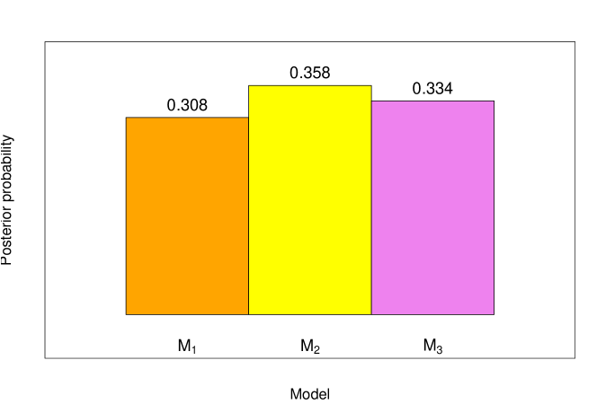
Figure 9: Posterior model probabilities. The prior probabilities have been chosen so that the models have approximately equal posterior probabilities.

Figure 10: Model trace indicator for the reversible jump algorithm.

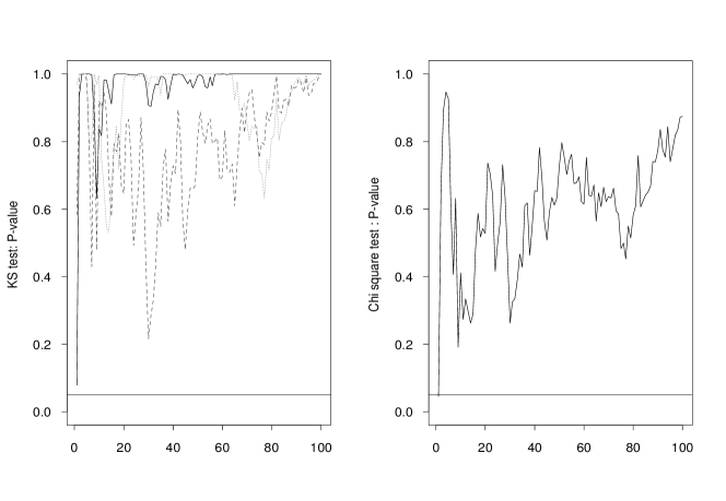
Figure 11: Convergence diagnostics.

The centering points used are the posterior means of the model parameters. For the scale parameters, we simulate those from their marginal posterior distributions, and then simulate the other proposal parameters conditional on this value of the scale parameter. The results clearly show the $\pi(M_{1}|\hbox{\boldmath$R$})\approx 1$, $\pi(M_{2}|\hbox{\boldmath$R$})\approx 0$, and $\pi(M_{3}|\hbox{\boldmath$R$})\approx 0$. To assess convergence of the algorithm, we simulate 3 chains using different starting values and different random number seeds for a total of 100000 iterations. Both the $\chi$-square and Kolmogorov–Smirnov diagnostics are computed. These diagnostics are plotted in Figure 11. In both cases, the diagnostic is well above the critical 5% value. The methods employed in this paper are not exactly weak non-identifiable centering methods. The approach that we use is general enough so that down moves, say from model $M_{1}$ to models $M_{2}$ or $M_{3}$, are not deterministic. This approach also allow the use of the posterior mean as the mean of or proposal density, from which the posterior variance matrix can be derived using the centering methods described.

9 Summary

Anova models arise in many areas of insurance credibility theory. The Bühlmann–Straub model can be reparameterised as a one–way model. In this paper, we use posterior model probabilities to compare one–way and two–way models. The results can be extended to cover yet more general models such as the jewell1975 and taylor1974 models. Using the conditional maximisation scheme of brooks2003, we constructed an algorithm which can be used to compute posterior model probabilities for model discrimination. When applied to loss ratios extracted from datasets of worker’s compensation insurance in the United States, there is overwhelming posterior odds in favour of the full model. This seems quite plausible given the structure and size of the data used. Model discrimination measures computed using the deviance information criterion, $DIC$, give results which are consistent with the reversible jump model probabilities obtained.

References

- [\citeauthoryearAhn, Chen, and LinAhn et al.1997] Ahn, H., J. J. Chen, and T. Lin (1997). A two–way analysis of covariance model for classification of stability data. Biometrical Journal 39(5), 559–576.
- [\citeauthoryearAl-Awadhi, Jennison, and HurnAl-Awadhi et al.2004] Al-Awadhi, F., C. Jennison, and M. Hurn (2004). Statistical image analysis for a confocal microscopy two–dimensional section of a cartilage growth. Journal of the Royal Statistical Society, Series C 53, 31–49.
- [\citeauthoryearAmit and GrenanderAmit and Grenander1991] Amit, Y. and U. Grenander (1991). Comparing sweep strategies for stochastic relaxation. Journal of Multivariate Analysis 37, 197–222.
- [\citeauthoryearBernardo and SmithBernardo and Smith1994] Bernardo, J. M. and A. F. M. Smith (1994). Bayesian Theory. Wiley.
- [\citeauthoryearBox and TiaoBox and Tiao1973] Box, G. E. P. and G. C. Tiao (1973). Bayesian inference in Statistical Analysis. Wiley Classics Library. Wiley.
- [\citeauthoryearBrooks, Giudici, and RobertsBrooks et al.2003] Brooks, S. P., P. Giudici, and G. O. Roberts (2003). Efficient construction of reversible jump MCMC proposal distributions (with discussion). Journal of the Royal Statistical Society, Series B 65(1), 3–55.
- [\citeauthoryearCarlin and ChibCarlin and Chib1995] Carlin, B. P. and S. Chib (1995). Bayesian Model Choice via Markov chain Monte Carlo methods. Journal of the Royal Statistical Society, Series B 57, 473–484.
- [\citeauthoryearCarlin and LouisCarlin and Louis1996] Carlin, B. P. and T. A. Louis (1996). Bayes and Empirical Bayes Methods for Data Analysis. Chapman and Hall.
- [\citeauthoryearClydeClyde1999] Clyde, M. A. (1999). Bayesian model averaging and model search strategies. In J. M. Bernardo, J. O. Berger, A. P. Dawid, and A. F. M. Smith (Eds.), Bayesian Statistics 6, pp. 157–185. Oxford University Press.
- [\citeauthoryearDannenburg, Kaas, and GoovaertsDannenburg et al.1996] Dannenburg, D. R., R. Kaas, and M. J. Goovaerts (1996). Practical Actuarial Credibility Models. University of Amsterdam: Institute for Actuarial Science.
- [\citeauthoryearEhlers and BrooksEhlers and Brooks2002] Ehlers, R. S. and S. P. Brooks (2002). Efficient Construction of Reversible Jump MCMC Proposals for ARMA Models. Technical report, Universidade Federal do Parana, Department de Estatistica.
- [\citeauthoryearGelfandGelfand1996a] Gelfand, A. E. (1996a). Efficient parametrizations for generalised linear mixed models (with discussion). In J. M. Bernardo, J. O. Berger, A. P. Dawid, and A. F. M. Smith (Eds.), Bayesian Statistics 5, pp. 165–180. Oxford University Press.
- [\citeauthoryearGelfandGelfand1996b] Gelfand, A. E. (1996b). Model determination using sampling-based methods. In W. R. Gilks, S. Richardson, and D. J. Spiegelhalter (Eds.), Markov chain Monte Carlo in Practice, pp. 145–161. Chapman and Hall.
- [\citeauthoryearGelfand, Carlin, and TrevisaniGelfand et al.2001] Gelfand, A. E., B. P. Carlin, and M. Trevisani (2001). On computation using Gibbs sampling for multilevel models. Statistica Sinica 11(4), 981–1003.
- [\citeauthoryearGelfand and SahuGelfand and Sahu1999] Gelfand, A. E. and K. Sahu (1999). Identifiability, improper priors, and Gibbs sampling for generalized linear models. Journal of the American Statistical Society 94(445), 247–253.
- [\citeauthoryearGelfand, Sahu, and CarlinGelfand et al.1995] Gelfand, A. E., S. K. Sahu, and B. P. Carlin (1995). Efficient Parametrisations for Normal Linear Mixed Models. Biometrika 82(3), 479–488.
- [\citeauthoryearGeorge and McCullochGeorge and McCulloch1993] George, E. I. and R. E. McCulloch (1993). Stochastic Search Variable Selection. Journal of the American Statistical Society 88, 881–889.
- [\citeauthoryearGilks and RobertsGilks and Roberts1996] Gilks, W. R. and G. O. Roberts (1996). Strategies for improving MCMC. In W. R. Gilks, S. Richardson, and D. J. Spiegelhalter (Eds.), Markov Chain Monte Carlo in Practice, pp. 89–114. Chapman and Hall.
- [\citeauthoryearGiudici and RobertsGiudici and Roberts1998] Giudici, P. and G. O. Roberts (1998). On the automatic choice of reversible jumps. In J. M. Bernardo, J. O. Berger, A. P. Dawid, and A. F. M. Smith (Eds.), Bayesian Statistics 6. Oxford University Press.
- [\citeauthoryearGodsillGodsill2001] Godsill, S. J. (2001). On the relationship between Markov chain Monte Carlo methods for model uncertainty. Journal of Computational and Graphical Statistics 10(2), 230–248.
- [\citeauthoryearGoovaerts and HoogstadGoovaerts and Hoogstad1987] Goovaerts, M. J. and W. J. Hoogstad (1987). Credibility Theory, Surveys of Actuarial Studies. Number 4 in Surveys of Actuarial Studies. Rotterdam: Nationale–Nederlanden.
- [\citeauthoryearGreenGreen1995] Green, P. J. (1995). Reversible jump Markov chain Monte Carlo computation and Bayesian model determination. Biometrika 82(4), 711–732.
- [\citeauthoryearGreenGreen2002] Green, P. J. (2002). Trans-dimensional Markov chain Monte Carlo. In Highly Structured Stochastic Systems, pp. 179–198. Oxford University Press.
- [\citeauthoryearGreen and MiraGreen and Mira2001] Green, P. J. and A. Mira (2001). Delayed rejection in reversible jump Metropolis–Hastings. Biometrika 88(4), 1035–1053.
- [\citeauthoryearGrenander and MillerGrenander and Miller1994] Grenander, U. and M. I. Miller (1994). Representations of knowledge in complex systems. Journal of the Royal Statistical Society, Series B 56, 549–603.
- [\citeauthoryearHills and SmithHills and Smith1992] Hills, S. E. and A. F. M. Smith (1992). Parameterization issues in Bayesian inference (with discussion). In J. M. Bernardo, A. F. M. Smith, A. P. Dawid, and J. O. Berger (Eds.), Bayesian Statistics 4, pp. 641–649. Oxford University Press.
- [\citeauthoryearHoeting, Madigan, Raftery, and VolinskyHoeting et al.1999] Hoeting, J. A., D. Madigan, A. E. Raftery, and C. T. Volinsky (1999). Bayesian model averaging. Statistical Science 14(4), 382–401.
- [\citeauthoryearHogg and KlugmanHogg and Klugman1984] Hogg, R. and S. A. Klugman (1984). Loss Distributions. New York: Wiley.
- [\citeauthoryearJewellJewell1975] Jewell, W. S. (1975). The use of collateral data in credibility theory: A hierarchical model. Giornale dell’Insituto Italiano degli Attuari 38, 1–16.
- [\citeauthoryearKey, Pericchi, and SmithKey et al.1999] Key, J. T., L. R. Pericchi, and A. F. M. Smith (1999). Bayesian Model Choice: What and Why. In J. M. Bernardo, J. O. Berger, A. P. Dawid, and A. F. M. Smith (Eds.), Bayesian Statistics 6, pp. 343–370. Oxford University Press.
- [\citeauthoryearKlugmanKlugman1987] Klugman, S. A. (1987). Credibility for classification ratemaking via the hierarchical normal linear model. Proceedings of the Casual Actuarial Society LXXIV, 272–321.
- [\citeauthoryearKlugmanKlugman1992] Klugman, S. A. (1992). Bayesian Statistics in Actuarial Science. Boston, MA: Kluwer Academic Publishers.
- [\citeauthoryearKremerKremer1982] Kremer, E. (1982). IBNR-Claims and the Two–Way Model of ANOVA. Scandinavian Actuarial Journal 1982(1), 47–55.
- [\citeauthoryearLedolter, Klugman, and LeeLedolter et al.1991] Ledolter, J., S. Klugman, and C.-S. Lee (1991). Credibility models with time-varying trend components. ASTIN Bulletin 21(1), 73–91.
- [\citeauthoryearLindley and SmithLindley and Smith1972] Lindley, D. V. and A. F. M. Smith (1972). Bayes estimates for the linear model. Journal of the Royal Statistical Society, Series B 4(1), 1–41.
- [\citeauthoryearLiu, Wong, and KongLiu et al.1994] Liu, J., W. Wong, and A. Kong (1994). Covariance structure of the Gibbs sampler with applications to the comparisons of estimators and augmentation schemes. Biometrika 81, 27–40.
- [\citeauthoryearMadigan and RafteryMadigan and Raftery1994] Madigan, D. and A. E. Raftery (1994). Model Selection and Accounting for Model Uncertainty in Graphical Models Using Occam’s Window. Journal of the American Statistical Society 89(428), 1535–1546.
- [\citeauthoryearNobile and GreenNobile and Green2000] Nobile, A. and P. J. Green (2000). Bayesian analysis of factorial experiments by mixture modelling. Biometrika 87(1), 15–35.
- [\citeauthoryearNorbergNorberg1986] Norberg, R. (1986). Hierarchical credibility: Analysis of a random effect linear model with nested classification. Scandinavian Actuarial Journal 1986, 204–222.
- [\citeauthoryearNtzoufras and DellaportasNtzoufras and Dellaportas2002] Ntzoufras, I. and P. Dellaportas (2002). Bayesian modelling of outstanding liabilities incorporating claim count uncertainty. North American Actuarial Journal 6(1), 113–128.
- [\citeauthoryearPapaspiliopoulos, Roberts, and SköldPapaspiliopoulos et al.2003] Papaspiliopoulos, O., G. O. Roberts, and M. Sköld (2003). Non-centered parameterizations for hierarchical models and data augmentation. In J. M. Bernardo, M. J. Bayarri, J. O. Berger, and A. P. Dawid (Eds.), Bayesian Statistics, Volume 7, pp. 307–326. Oxford University Press.
- [\citeauthoryearPhillips and SmithPhillips and Smith1996] Phillips, D. B. and A. F. M. Smith (1996). Bayesian model comparison via jump diffusions. In W. R. Gilks, S. Richardson, and D. J. Spiegelhalter (Eds.), Markov Chain Monte Carlo in Practice, pp. 215–239. Chapman and Hall.
- [\citeauthoryearRamlau-HansenRamlau-Hansen1982] Ramlau-Hansen, H. (1982). An Application of Credibility Theory to Solvency Margins. Some comments on a Paper by G. W. De Wit and W. M. Kastelijn. ASTIN Bulletin 13(1), 37–45.
- [\citeauthoryearRoberts and SahuRoberts and Sahu1997] Roberts, G. O. and S. K. Sahu (1997). Updating schemes, correlation structure, blocking and parametrization for the Gibbs sampler. Journal of the Royal Statistical Society, Series B 59(2), 291–317.
- [\citeauthoryearRotondiRotondi2002] Rotondi, R. (2002). On the influence of the proposal distributions on a reversible jump MCMC algorithm applied to the detection of multiple change–points. Computational Statistics and Data Analysis 40(3), 633–653.
- [\citeauthoryearRubinRubin1995] Rubin, D. (1995). Discussion of “Fractional Bayes Factors for Model Comparison” by A. O’Hagan. Journal of the Royal Statistical Society, Series B 57(1), 133.
- [\citeauthoryearSchefféScheffé1959] Scheffé, H. (1959). The Analysis of Variance. New York: Wiley.
- [\citeauthoryearSmithSmith1973] Smith, A. F. M. (1973). Bayes Estimates in One-Way and Two-Way Models. Biometrika 60(2), 319–329.
- [\citeauthoryearSpiegelhalter, Best, Carlin, and van der LindeSpiegelhalter et al.2002] Spiegelhalter, D. J., N. G. Best, B. P. Carlin, and A. van der Linde (2002). Bayesian measures of model complexity and fit. Journal of the Royal Statistical Society, Series B 64(3), 1–34.
- [\citeauthoryearStephensStephens2000] Stephens, M. (2000). Bayesian analysis of mixture models with an unknown number of components-an alternative to reversible jump methods. Annals of Statistics 28(1), 40–74.
- [\citeauthoryearTaylorTaylor1974] Taylor, G. C. (1974). Experience rating with credibility adjustment of the manual premium. ASTIN Bulletin 7(3), 323–336.
- [\citeauthoryearTaylorTaylor1979] Taylor, G. C. (1979). Credibility analysis of a general hierarchical model. Scandinavian Actuarial Journal 1979, 1–12.
- [\citeauthoryearTroughton and GodsillTroughton and Godsill1997] Troughton, P. T. and S. J. Godsill (1997). A reversible jump sampler for autoregressive time series, employing full conditionals to achieve efficient model space moves. Technical report, Department of Engineering, University of Cambridge, Signal Processing and Communications Laboratory.
- [\citeauthoryearVehtariVehtari2002] Vehtari, A. (2002). Discussion of “Bayesian measures of model complexity and fit”. Journal of the Royal Statistical Society, Series B 64(4), 620.
- [\citeauthoryearVehtari and LampinenVehtari and Lampinen2002] Vehtari, A. and J. Lampinen (2002). Bayesian model assessment and comparison using cross–validation predictive densities. Neural Computation 14(10), 2439–2468.
- [\citeauthoryearVenables and RipleyVenables and Ripley1999] Venables, W. N. and B. D. Ripley (1999). Modern Applied Statistics with S-Plus (Third ed.). Springer.
- [\citeauthoryearWhittakerWhittaker1990] Whittaker, J. (1990). Graphical models in applied multivariate statistics. Chichester: Wiley.
- [\citeauthoryearZehnwirthZehnwirth1982] Zehnwirth, B. (1982). Conditional linear Bayes rules for hierarchical models. Scandinavian Actuarial Journal 1982, 143–154.