Light Cone Sum Rules for the $\pi^{0}\gamma^{*}\gamma$ Form Factor Revisited

Abstract

We provide a theoretical update of the calculations of the $\pi^{0}\gamma^{*}\gamma$ form factor in the LCSR framework, including up to six polynomials in the conformal expansion of the pion distribution amplitude and taking into account twist-six corrections related to the photon emission at large distances. The results are compared with the calculations of the $B\to\pi\ell\nu$ decay and pion electromagnetic form factors in the same framework. Our conclusion is that the recent BaBar measurements of the $\pi^{0}\gamma^{*}\gamma$ form factor at large momentum transfers BABAR are consistent with QCD, although they do suggest that the pion DA may have more structure than usually assumed.

I Introduction

Despite a solid theory background Chernyak:1977as ; Radyushkin:1977gp ; Lepage:1979zb , phenomenological success of QCD in exclusive reactions has been rather modest. A problem is that, since the quarks carry only some fractions of hadron momenta, virtualities of the internal lines of the hard subprocess appear to be essentially smaller than $Q^{2}$, the nominal momentum transfer to the hadron. As a result, at accessible $Q^{2}$, the bulk part of the hard QCD contribution comes from the regions where the “hard” virtualities are much smaller than the typical hadronic scale of 1 GeV² Efremov:1980mb ; Isgur:1988iw ; Radyushkin:1990te . According to the factorization principle, contributions from such regions have to be subtracted from the hard coefficient function and included separately as additive “soft” or “end-point” nonperturbative contributions. The standard power counting suggests that “soft” terms are suppressed by extra powers of $1/Q^{2}$. However, they do not involve small coefficients $\sim\alpha_{s}(Q)/\pi$ which are endemic for factorizable QCD contributions based on hard gluon exchanges. As the result, the onset of the perturbative regime may be postponed to very large momentum transfers.

The pion transition form factor ${\gamma^{*}\gamma^{(*)}\to\pi^{0}}$ with at least one virtual photon plays a very special rôle as it is the simplest hard exclusive process where the above mentioned difficulties are absent or, at least, moderated. There is only one hadron (pion) involved, and the large $Q^{2}$ behavior of this form factor is determined Lepage:1979zb by the operator product expansion (OPE) of the product of two electromagnetic currents near the light cone which is very well studied in the context of inclusive deep-inelastic scattering (DIS). In this case the leading contribution to the hard coefficient function is of order one (i.e. not suppressed) as no gluon exchanges are involved, and at the same time “soft” (end-point) contributions either do not exist — for the case of two virtual photons — or are likely to be suppressed, if one photon is real. These features make the pion transition form factor an ideal place to test the QCD factorization approach and determine the pion distribution amplitude (DA) which can then be used to describe other exclusive hard reactions. This task is as important as ever, the most high-profile application being at present to exclusive weak $B$-decays, $B\to\pi\ell\nu_{\ell}$, $B\to\pi\pi$ etc. which are the main source of precision information on quark flavor mixing parameters in the Standard Model. These are the aim of an extensive experimental study: It addresses the question whether there is New Physics in flavor-changing processes and where it manifests itself.

Whereas the case of two virtual photons offers crucial simplifications for the theory, the transition form factors with one real and one virtual photon are much easier to study experimentally. They can be measured for space-like momentum transfers in the process $e^{+}e^{-}\to e^{+}e^{-}\pi^{0},\eta,\ldots$ and in $e^{+}e^{-}\to\gamma\pi^{0},\eta,\ldots$ for time-like ones. Till 1995 only the CELLO data Behrend:1990sr were available at relatively low, space-like momentum transfer: $Q^{2}<2.5$ GeV² for $\pi^{0}(\eta)\gamma^{*}\gamma$ and somewhat higher for $\eta^{\prime}\gamma^{*}\gamma$. The covered region was extended to $Q^{2}\sim 9-15$ GeV² by CLEO collaboration Gronberg:1997fj which allowed, for the first time, a quantitative comparison with the perturbative QCD. The CLEO data appeared to be consistent with the predicted scaling behavior $\sim 1/Q^{2}$ setting in for momentum transfers of the order of a few GeV² and also suggested that the pion DA is somewhat broader compared to its asymptotic shape at large scales, which was, again, expected based on the corresponding studies using QCD sum rules. More recently, BaBar reported Aubert:2006cy a measurement of the time-like transition form factors $\eta\gamma^{*}\gamma$ and $\eta^{\prime}\gamma^{*}\gamma$ at very large $q^{2}=112$ GeV². No significant tension with the theory was observed, although predictions in the time-like region are generally more difficult.

The situation changed in 2009 when the BaBar collaboration presented BABAR the measurement of the $\pi^{0}\gamma^{*}\gamma$ form factor up to photon virtualities of the order of 40 GeV². These new data created considerable excitement in the theory community as they do not show the expected scaling behavior. The most popular explanation so far has been Radyushkin:2009zg ; Polyakov:2009je that the pion DA has an unexpected “flat” shape and does not vanish at the end points. This, on one hand, triggered speculations on the breakdown of QCD factorization Dorokhov:2010bz and, on the other hand, claims that the BaBar data are in contradiction with light-cone sum rules (LCSRs) and with the common wisdom on the lowest moments of the pion DA Mikhailov:2009kf ; Mikhailov:2010aq ; Mikhailov:2010ud . The aim of this work is to reexamine these claims by making an updated analysis of the $\pi^{0}\gamma^{*}\gamma$ form factor within the LCSR approach including up to six polynomials in the conformal expansion of the pion distribution amplitude and taking into account twist-six corrections. The photon emission at large distances is discussed in detail. The results are compared with the calculations of pion electromagnetic form factor and $B\to\pi\ell\nu$ decay in the same framework. Our conclusion is that the recent BaBar measurements BABAR are consistent with QCD and with the bulk of the available information on the pion distribution amplitude. In particular we argue that the “flat” DA Radyushkin:2009zg ; Polyakov:2009je is not warranted and in fact no conclusion on the end–point behavior of the DA can be inferred on the basis of the existing experimental data.

The presentation is organized as follows. Sect. 2 contains a concise review of the QCD (collinear) factorization approach to the $\pi^{0}\gamma^{*}\gamma$ form factor and the existing information on the pion DA. The LCSR approach is motivated and explained in detail in Sect. 3. In this work we go beyond the existing analysis Khodjamirian:1997tk ; Schmedding:1999ap ; Bakulev:2001pa ; Bakulev:2002uc ; Bakulev:2003cs ; Agaev:2005rc ; Mikhailov:2009kf in two aspects. First, we calculate a new, twist-six contribution to LCSRs which proves to be sizeable. This contribution is related to photon emission from large distances for which we also derive the leading-order perturbative expression. Second, we extend the existing formalism to allow for the contributions of higher-order Gegenbauer polynomials, which allows one to consider DAs of arbitrary shape and also address the question of convergence of the Gegenbauer expansion which generated some confusion. The second task was already addressed in Ref. Mikhailov:2009kf , but our expressions do not agree, unfortunately. Sect. 4 contains the numerical study of the LCSRs to the NLO accuracy. We consider various uncertainties of the method in some detail and provide error estimates for our predictions. The final Sect. 5 is reserved for a summary and conclusions.

II QCD factorization and pion DA

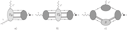
Figure 1: Schematic structure of the QCD factorization for the $F_{\gamma^{*}\gamma\to\pi^{0}}(Q^{2})$ factor factor.

The form factor $F_{\gamma^{*}\gamma^{*}\to\pi^{0}}(q_{1}^{2},q_{2}^{2})$ describing the pion transition in two (in general virtual) photons can be defined by the matrix element of the product of two electromagnetic currents

$$\int d^{4}ye^{iq_{1}y}\langle\pi^{0}(p)|T\{j^{\rm em}_{\mu}(y)j^{\rm em}_{\nu}(0)\}|0\rangle=$$ (1)

$$\hskip 42.67912pt=\,ie^{2}\varepsilon_{\mu\nu\alpha\beta}q_{1}^{\alpha}q_{2}^{\beta}F_{\gamma^{*}\gamma^{*}\to\pi^{0}}(q_{1}^{2},q_{2}^{2})$$

where

$$j^{\rm em}_{\mu}(y)=e_{u}\bar{u}(y)\gamma_{\mu}u(y)+e_{d}\bar{d}(y)\gamma_{\mu}d(y)+\ldots,$$

$p$ is the pion momentum and $q_{2}=q_{1}+p$. We will consider the space-like form factor, in which case the both photon virtualities are negative. The experimentally relevant situation is when one virtuality is large and the second one small (or zero). For definiteness we take

$$q_{1}^{2}=-Q^{2}\,,\qquad q_{2}^{2}=-q^{2}\,,$$ (2)

assuming that $q^{2}\ll Q^{2}$. Most of the equations are written for $q^{2}=0$ and we use a shorthand notation $F_{\gamma^{*}\gamma\to\pi^{0}}(Q^{2})\equiv F_{\gamma^{*}\gamma^{*}\to\pi^{0}}(q_{1}^{2}=-Q^{2},q^{2}=0)$.

In general, a power-like falloff of the form factor $F_{\gamma^{*}\gamma\to\pi^{0}}(Q^{2})$ in the large-$Q^{2}$ limit can be generated by the three different possibilities of the large-momentum flow as indicated schematically in Fig. 1 Musatov:1997pu . The first possibility, Fig. 1a, corresponds to the hard subgraph that includes both photon vertices. This is the dominant contribution that starts at order $\sim 1/Q^{2}$. For zero (or small, $q^{2}\leq\Lambda^{2}_{\rm QCD}$) virtuality of the second photon there exists another possibility shown in Fig. 1b: In this case the low-virtual photon is emitted at large distances and the large momentum flows through a subgraph corresponding to hard gluon exchange between the quarks. The power counting for this contribution shows that it is at most ${\mathcal{O}}(1/Q^{4})$, i.e. subleading compared to the first regime. Finally, the third possible regime shown in Fig. 1c corresponds to the Feynman mechanism, i.e. the possibility that the quark interacting with the hard photon carries almost all the momentum whereas the quark spectator is soft. This contribution can intuitively be thought of as an overlap of nonperturbative wave functions describing the initial (photon) and final (pion) states. In perturbation theory, this contribution also scales as ${\mathcal{O}}(1/Q^{4})$ in the large-$Q^{2}$ limit.

The contribution in Fig. 1a by construction involves a time-ordered product of two electromagnetic currents at small light-cone separations. Hence it can be studied using Wilson operator product expansion. The leading contribution ${\mathcal{O}}(1/Q^{2})$ to the form factor corresponds to the contribution of the leading twist-two operators and can be written in the factorized form

$$F_{\gamma^{*}\gamma\to\pi^{0}}(Q^{2})=\frac{\sqrt{2}f_{\pi}}{3}\!\int_{0}^{1}\!dx\,T_{H}(x,Q^{2},\mu,\alpha_{s}(\mu))\phi_{\pi}(x,\mu)\,,$$ (3)

where $\phi_{\pi}(x,\mu)$, the pion distribution amplitude at the scale $\mu$, is defined by the matrix element of the nonlocal quark-antiquark operator stretched along the light-like direction $n_{\mu}$, $n^{2}=0$:

$$\langle 0|\bar{q}(0)[0,\alpha n]\not\!n\gamma_{5}q(\alpha n)|\pi^{+}(p)\rangle=$$ (4)

$$\hskip 14.22636pt=\,if_{\pi}p\cdot n\int_{0}^{1}dx\,e^{-ix\alpha p\cdot n}\,\phi_{\pi}(x,\mu)\,.$$

Here and below $\bar{q}\,\not{n}\gamma_{5}q=(1/\sqrt{2})[\bar{u}\,\not{n}\gamma_{5}u-\bar{d}\,\not{n}\gamma_{5}d]$. To this accuracy (leading twist) all gluon attachments to the hard subgraph (cf. Fig. 1a) can be absorbed in the path-ordered gauge link (Wilson line):

$$[0,\alpha n] = ~{}\mbox{\rm Pexp}\left\{-ig\int_{0}^{\alpha}du\,n^{\mu}A_{\mu}(un)\right\}.$$ (5)

The normalization is such that

$$\langle 0|\bar{q}(0)\gamma_{\nu}\gamma_{5}q(0)|\pi^{0}(p)\rangle\,=\,if_{\pi}p_{\nu}\,,\quad\int_{0}^{1}dx\,\phi_{\pi}(x,\mu)\,=\,1\,,$$ (6)

where $f_{\pi}\simeq 131$ MeV is the usual pion decay constant.

The coefficient function in (3) is known in the $\overline{MS}$ scheme to the next-to-leading order (NLO) in the strong coupling delAguila:1981nk ; Braaten:1982yp ; Kadantseva:1985kb . Taking into account the symmetry of the pion DA $\phi_{\pi}(x)=\phi_{\pi}(1-x)$ it can be written as

$$T_{H}^{\rm NLO} = \frac{1}{xQ^{2}}\Big{\{}1+C_{F}\frac{\alpha_{s}(\mu)}{2\pi}\Big{[}\frac{1}{2}\ln^{2}x-\frac{x\ln x}{2(1-x)}$$ (7)

$${}-\frac{9}{2}+\left(\frac{3}{2}+\ln x\right)\ln\frac{Q^{2}}{\mu^{2}}\Big{]}\Big{\}}.$$

Symmetry properties of the renormalization-group (RG) equation which governs the scale dependence of the pion DA Radyushkin:1977gp ; Lepage:1979zb suggest the series expansion of the DA in Gegenbauer polynomials

$$\phi_{\pi}(x,\mu) = \sum_{n=0}^{\infty}a_{n}(\mu)\,\varphi_{n}(x)\,,$$

$$\varphi_{n}(x) = 6x(1-x)C_{n}^{3/2}(2x-1)\,.$$ (8)

The first coefficient $a_{0}(\mu)=1$ is fixed by the normalization condition whereas the remaining ones, $a_{n}(\mu_{0})$ for $n=2,4,\ldots$, have to be determined by some nonperturbative method (or taken from experiment).

To leading order (LO) the Gegenbauer coefficients are renormalized multiplicatively whereas to the NLO accuracy the mixing pattern becomes more complicated. One obtains Dittes:1983dy ; Sarmadi:1982yg ; Katz:1984gf ; Mikhailov:1984ii ; Mueller:1993hg ; Mueller:1994cn

$$a^{\rm NLO}_{n}(\mu) = a_{n}(\mu_{0})\,E^{\rm NLO}_{n}(\mu,\mu_{0})$$ (9)

$${}+\frac{\alpha_{s}(\mu)}{4\pi}\sum_{k=0}^{n-2}a_{k}(\mu_{0})\,E^{\rm LO}_{k}(\mu,\mu_{0})\,d_{n}^{k}(\mu,\mu_{0})\,,$$

Explicit expressions for the RG factors $E^{\rm(N)LO}_{n}(\mu,\mu_{0})$ and the off-diagonal mixing coefficients $d_{n}^{k}(\mu,\mu_{0})$ in the $\overline{\rm MS}$ scheme are collected in Appendix A.

The NNLO calculations of the transition pion form factor exist in the so-called conformal scheme $\overline{\rm CS}$ Melic:2002ij ; Braun:2007wv but they cannot be converted to $\overline{\rm MS}$ lacking the full NNLO result for the trace anomaly term, which is so far not available. An extensive discussion of scheme dependence can be found in Refs. Mueller:1993hg ; Mueller:1994cn ; Melic:2002ij .

The existing information on the pion DA comes from QCD sum rules, lattice calculations and light-cone sum rules. The first nontrivial Gegenbauer coefficient $a_{2}$ is related to the second moment of the DA

$$\langle\xi^{2}\rangle\equiv\int_{0}^{1}dx\,(2x-1)^{2}\phi_{\pi}(x)\,,\qquad a_{2}=\frac{7}{12}\big{(}5\langle\xi^{2}\rangle-1\big{)}$$ (10)

and can be evaluated as a matrix element of the local operator with two derivatives between vacuum and the pion state. There exists overwhelming evidence that this coefficient is positive, meaning that the pion DA is broader than its asymptotic expression $\phi_{\pi}^{\rm as}=6x(1-x)$, see Table 1.

Method	$\mu=1$ GeV	$\mu=2$ GeV	Reference
LO QCDSR, CZ model	$0.56$	$0.39$	Chernyak:1981zz ; CZreport
QCDSR	$0.26^{+0.21}_{-0.09}$	$0.18^{+0.15}_{-0.06}$	Khodjamirian:2004ga
QCDSR	$0.28\pm 0.08$	$0.19\pm 0.06$	Ball:2006wn
QCDSR, NLC	$0.19\pm 0.06$	$0.13\pm 0.04$	Mikhailov:1991pt ; Bakulev:1998pf ; Bakulev:2001pa
$F_{\pi\gamma\gamma^{*}}$, LCSR	$0.19\pm 0.05$	$0.12\pm 0.03$  $(\mu=2.4)$	Schmedding:1999ap
$F_{\pi\gamma\gamma^{*}}$, LCSR	$0.32$	$0.21$ $(\mu=2.4)$	Bakulev:2002uc
$F_{\pi\gamma\gamma^{*}}$, LCSR, R	$0.44$	$0.31$	Bakulev:2005cp
$F_{\pi\gamma\gamma^{*}}$, LCSR, R	$0.27$	$0.19$	Agaev:2005rc
$F^{\rm em}_{\pi}$,LCSR	$0.24\pm 0.14\pm 0.08$	$0.17\pm 0.10\pm 0.05$	Braun:1999uj ; Bijnens:2002mg
$F^{\rm em}_{\pi}$,LCSR, R	$0.20\pm 0.03$	$0.14\pm 0.02$	Agaev:2005gu
$F_{B\to\pi\ell\nu}$, LCSR	$0.19\pm 0.19$	$0.13\pm 0.13$	Ball:2005tb
$F_{B\to\pi\ell\nu}$, LCSR	$0.16$	$0.11$	Duplancic:2008ix
LQCD, $N_{f}=2$, CW	$0.289\pm 0.166$	$0.201\pm 0.114$	QCDSF/UKQCD Braun:2006dg
LQCD, $N_{f}=2\!+\!1$, DWF	$0.334\pm 0.129$	$0.233\pm 0.088$	RBS/UKQCD Donnellan:2007xr

Table 1: The Gegenbauer moment $a_{2}(\mu^{2})$. The CZ model involves $a_{2}=2/3$ at the low scale $\mu=500$ MeV; for the discussion of the extrapolation to higher scales, see Ref. Bakulev:2002uc . The abbreviations stand for: QCDSR: QCD sum rules; NLC: non-local condensates; LCSR: light-cone sum rules; R: renormalon model for twist-4 corrections; LQCD: lattice calculation; $N_{f}=2(+1)$: calculation using $N_{f}=2(+1)$ dynamical quarks; CW: non-perturbatively ${\mathcal{O}}(a)$ improved Clover–Wilson fermion action; DWF: domain wall fermions. For convenience we present the results for two scales, $\mu=1$ GeV and $\mu=2$ GeV, the relation is calculated in NLO.

Such calculations where pioneered in 1981 by Chernyak and Zhitnitsky Chernyak:1981zz who derived the corresponding sum rule and obtained $a_{2}\sim 0.5$ at the scale of order $\mu^{2}=1-1.5$ GeV². Extrapolating this number to a very low scale $\mu^{2}=0.25$ GeV² and adding a simplifying assumption that higher-order coefficients $a_{4},\ldots$ vanish, they have formulated a simple model for the low-energy pion DA, which has become known as the Chernyak-Zhitnitsky (CZ) model:

$$\phi^{\rm CZ}_{\pi}(x) = 30x(1-x)(2x-1)^{2}$$ (11)

$$= 6x(1-x)\left[1+\frac{2}{3}C_{2}^{3/2}(2x-1)\right].$$

This model corresponds to a very asymmetric momentum fraction distribution which vanishes at the point where the pion momentum is shared equally between the quark and the antiquark $\phi^{\rm CZ}_{\pi}(x=1/2)=0$. The striking difference of the CZ model and the asymptotic DA has been fuelling an extensive and sometimes heated discussion for many years.

Newer estimates of $a_{2}$ following the CZ approach yield a somewhat smaller value Khodjamirian:2004ga ; Ball:2006wn $a_{2}(1$ GeV$)\sim 0.3$, the difference being due to a combination of several factors: writing the sum rules for $a_{2}$ directly instead of the second moment $\langle\xi^{2}\rangle$, taking into account the NLO corrections and using slightly different values of the parameters.

Light-cone sum rules Balitsky:1989ry ; Braun:1988qv ; Chernyak:1990ag are a modification of the general SVZ approach SVZ , in which the pion DA serves as the main input in calculations of form factors (or hadron matrix elements). The Gegenbauer coefficient $a_{2}$ is not calculated directly, but is extracted from the comparison of the LCSR calculations with the experimental data. Note that in the case of the pion transition form factor these fits are based on CLEO data Gronberg:1997fj only. The results for $a_{2}$ are consistent with the direct calculations, see Table 1.

Finally, two independent lattice calculations of $a_{2}$ are now available Braun:2006dg ; Donnellan:2007xr . The largest part of the uncertainty in these results is due to the chiral extrapolation. Overall, the results in Table 1 show a consistent picture

$$a^{\rm NLO}_{2}(\mu^{2}=1~{}\mbox{GeV}^{2})=0.25\pm 0.10$$ (12)

and one can expect that the accuracy will increase in near future when lattice calculations with physical pion mass become available.

Very little, unfortunately, is known about the next Gegenbauer coefficient, $a_{4}$. The LCSR fits of heavy meson decay form factors indicate a small positive value, $a_{4}\sim 0.04$ Duplancic:2008ix , whereas the similar approach applied to pion transition form factor (CLEO data only) favors small negative values Bakulev:2002uc ; Bakulev:2005cp ; Agaev:2005rc . Lattice calculations of this coefficient suffer from large (lattice) artifacts in the operator renormalization and are not feasible at present.

The calculation of $a_{4}$ within the QCD sum rule approach has been attempted in the so-called nonlocal condensate model (NLC) Mikhailov:1991pt ; Bakulev:1998pf ; Bakulev:2001pa which involves a resummation of a tower of condensates of a certain type. This approach leads to a sizeable negative value $a_{4}\sim-0.1$ which is included in the so-called Bakulev-Mikhailov-Stefanis (BMS) model of the pion DA. A large negative value for $a_{4}$ in the NLC approach can be traced back to the basic feature of this model that nonperturbative corrections to the DA get smeared over a finite interval of momentum fractions $\Delta x\sim\lambda_{q}^{2}/(2M^{2})\sim 0.2$ where $\lambda^{2}_{q}=\langle\bar{q}D^{2}q\rangle/\langle\bar{q}q\rangle\sim 0.4$ GeV² is the average virtuality of quarks in QCD vacuum and $M^{2}\sim 1$ GeV² is the Borel parameter. To our opinion, appearance of $\Delta x$ is an artifact of the NLC model: contributions of this type would produce “bumps” at large values of Bjorken variable in quark parton distributions in the nucleon Braun:1994jq (which are absent) and also a finite smearing proves not sufficient to cure the QCD sum rules for heavy-to-light decay form factors Ali:1993vd (which is the reason why this technique was eventually abandoned and replaced by LCSRs). It seems much more natural to assume that the nonperturbative contributions get smeared over the whole interval of momentum fractions $0<x<1$. A possible mechanism for such “complete” smearing is considered on the example of a photon DA in Appendix B in Ref. Ball:2002ps . We believe, therefore, that the NLC-model-based predictions for $a_{4}$ have to be viewed with caution.

Last but not least, we mention the LCSR calculation Braun:1988qv for the pion DA in the middle point:

$$\phi_{\pi}(x=0.5,\mu^{2}=1~{}\mbox{GeV}^{2})=1.2\pm 0.3\,,$$ (13)

which is only available result beyond the Gegenbauer expansion. This result excludes a large “dip” in the pion DA in the center region and thus contradicts the CZ and BMS models. It is, however, consistent with most of the parameterizations of the pion DA that are used in vast literature on $B$-decays. Smaller values of $\phi_{\pi}(x=0.5)$ are also strongly disfavored by numerous LCSR calculations of pion-hadron couplings $g_{\pi NN},g_{\pi DD^{*}},g_{\rho\omega\pi},\ldots$, see e.g. Braun:1988qv ; Belyaev:1994zk ; Khodjamirian:1999hb ; Aliev:1999ce ; Aliev:2006xr ; Aliev:2009kg .

It has been suggested Radyushkin:2009zg ; Polyakov:2009je that the BaBar data BABAR indicate an unusual “flat” DA $\phi_{\pi}(x)\simeq 1$ which does not vanish at the end points so that the Gegenbauer expansion is not convergent (more precisely: not uniformly convergent at the end points). We believe that this conclusion is not warranted and in fact no conclusion on the end–point behavior of the pion DA can be inferred on the basis of the existing experimental data.

To explain our statement, let us examine the argumentation in Radyushkin:2009zg more closely. It is based on the elegant model for the transition form factor suggested by Musatov and Radyushkin (MR) in an earlier work Musatov:1997pu , which is derived from the exact two-body (e.g. quark-antiquark) contribution in the noncovariant light-cone formalism of Brodsky and Lepage Lepage:1979zb under certain simplifying assumptions on the shape of the pion wave function:

$$F^{\rm MR}_{\gamma^{*}\gamma\to\pi^{0}}(Q^{2})=\frac{\sqrt{2}f_{\pi}}{3Q^{2}}\int_{0}^{1}\!\frac{dx}{x}\phi_{\pi}(x)\left[1-\exp\left(-\frac{xQ^{2}}{2\bar{x}\sigma}\right)\right].$$ (14)

The first term in the square brackets corresponds to the usual leading-order contribution to Fig. 1a, whereas the second term is entirely a soft contribution of the type Fig. 1c. Note that this second term is exponentially small in $Q^{2}$ for each finite quark momentum fraction, so it is absent in any order of the operator product expansion. Using Eq. (14) with $\sigma=0.53~{}\mbox{GeV}^{2}$ Radyushkin:2009zg and the “flat” pion DA $\phi_{\pi}(x)=1$ allows one to describe the apparent scaling violation in the BaBar data, as illustrated by the solid curve in Fig. 2.

Figure 2: Pion transition form factor in the MR model (14) calculated using flat pion DA (solid red curve) and CZ-type DA with $a_{2}=0.5$ and higher Gegenbauer moments set to zero (dashed blue curve). The nonperturbative parameter $\sigma=0.53~{}\mbox{GeV}^{2}$ in both cases. The experimental data are from BABAR (full circles) and Gronberg:1997fj (open triangles).

The caveat with this argument (and a very similar argumentation in Ref. Polyakov:2009je ) is that flat DA is not necessary; in fact a CZ-type DA with $a_{2}=0.5$

$$\phi_{\pi}(x)=6x(1-x)\left[1+\frac{1}{2}C_{2}^{3/2}(2x-1)\right]$$

yields a very similar (or even better) description of the data, see the dashed (blue) curve in the same figure. Moreover, it is seen that the two DA models can hardly be discriminated at all unless precise data with $Q^{2}>20$ GeV² are available!

It is easy to see why this happens. The flat DA $\phi^{\rm flat}_{\pi}(x)=1$ can be expanded in Gegenbauer polynomials as follows:

$$1=\sum_{k=0,2,\ldots}a_{k}^{\rm flat}\varphi_{k}(x)\,,\qquad a_{k}^{\rm flat}\,=\,\frac{2(2k+3)}{3(k+1)(k+2)}\,.$$ (15)

This equation has to be understood in the sense of distributions: The equality holds when both sides are integrated with a test function that is finite (or does not increase too fast) at the end points.

In perturbation theory (LO) the form factor is proportional to the sum of the Gegenbauer coefficients

$$\int_{0}^{1}\!\frac{dx}{x}\phi_{\pi}(x)=3\Big{[}1+a_{2}+a_{4}+\ldots\Big{]}\,.$$

For the flat DA this series diverges, which motivates introduction of a certain regulator, e.g. the soft correction given by second, exponential, term in Eq. (14) or effective quark mass in Ref. Polyakov:2009je . Our observation is, however, that if such a regulator is included, the Gegenbauer expansion for the form factor is converging very rapidly and contributions of higher-order terms in this series are in fact negligible. For illustration, consider the MR model with a flat DA for, say $Q^{2}=20$ GeV², and check how much is being contributed by each successive Gegenbauer polynomial. One obtains

$$Q^{2}F^{\rm MR,flat}_{\gamma^{*}\gamma\to\pi^{0}}(Q^{2}=20) = \frac{\sqrt{2}f_{\pi}}{3}\cdot 3.56513$$ (16)

$${}=\frac{\sqrt{2}f_{\pi}}{3}\Big{[}2.724+0.649+0.162+0.028+\ldots\Big{]}$$

where the first term on the r.h.s. is the contribution of the asymptotic DA, the second term is due to $a^{\rm flat}_{2}$ etc. One sees that all contributions beyond $n=4$ are tiny.

Our conclusion is that a good description of the BaBar data BABAR achieved in Radyushkin:2009zg ; Polyakov:2009je is not due to an unusual end-point behavior of the DA, but rather to a (model dependent) large nonperturbative soft correction to the form factor. Such a large correction effectively suppresses contributions of higher order terms in the Gegenbauer expansion and makes the question of the end-point behavior of the pion DA irrelevant. The problem is, therefore, whether such a large nonperturbative correction can be expected, and whether it can be estimated in a model-independent way. This is the question that we address in the next Section.

III Light Cone Sum Rules for the pion-photon transition

III.1 Dispersion approach

The technique that we adopt in what follows has been suggested originally by Khodjamirian in Khodjamirian:1997tk . It is to calculate the pion transition form factor for two large virtualities, $Q^{2}$ and $q^{2}$, using the OPE, and make the analytic continuation to the real photon limit $q^{2}=0$ using dispersion relations. In this way explicit evaluation of contributions of the type in Fig. 1b,c is avoided (since they do not contribute for sufficiently large $q^{2}$) and effectively replaced by certain assumptions on the physical spectral density in the $q^{2}$-channel.

The starting observation Khodjamirian:1997tk is that $F_{\gamma^{*}\gamma^{*}\to\pi^{0}}(Q^{2},q^{2})$ satisfies an unsubtracted dispersion relation in the variable $q^{2}$ for fixed $Q^{2}$. Separating the contribution of the lowest-lying vector mesons $\rho,\omega$ one can write

$$F_{\gamma^{*}\gamma^{*}\to\pi^{0}}(Q^{2},q^{2}) = \frac{\sqrt{2}f_{\rho}F_{\gamma^{*}\rho\to\pi^{0}}(Q^{2})}{m^{2}_{\rho}+q^{2}}$$ (17)

$${}+\frac{1}{\pi}\int_{s_{0}}^{\infty}ds\,\frac{\mathrm{Im}F_{\gamma^{*}\gamma^{*}\to\pi^{0}}(Q^{2},-s)}{s+q^{2}}$$

where $s_{0}$ is a certain effective threshold. Here, the $\rho$ and $\omega$ contributions are combined in one resonance term assuming $m_{\rho}\simeq m_{\omega}$ and the zero-width approximation is adopted; $f_{\rho}\sim 200$ MeV is the usual vector meson decay constant. Note that since there are no massless states, the real photon limit is recovered by the simple substitution $q^{2}\to 0$ in (17).

On the other hand, the same form factor can be calculated using QCD perturbation theory and the OPE. The QCD result satisfies a similar dispersion relation

$$F^{\rm QCD}_{\gamma^{*}\gamma^{*}\to\pi^{0}}(Q^{2},q^{2})=\frac{1}{\pi}\int_{0}^{\infty}ds\,\frac{\mathrm{Im}F^{\rm QCD}_{\gamma^{*}\gamma^{*}\to\pi^{0}}(Q^{2},-s)}{s+q^{2}}\,.$$ (18)

The basic assumption of the method is that the physical spectral density above the threshold $s_{0}$ coincides with the QCD spectral density as given by the OPE:

$$\mathrm{Im}F_{\gamma^{*}\gamma^{*}\to\pi^{0}}(Q^{2},-s)=\mathrm{Im}F^{QCD}_{\gamma^{*}\gamma^{*}\to\pi^{0}}(Q^{2},-s)$$ (19)

for $s>s_{0}$. This is the usual approximation of local quark-hadron duality.

We expect that the QCD result reproduces the “true” form factor for large values of $q^{2}$. Equating the two representations (17),(18) at $q^{2}\to-\infty$ and subtracting the contributions of $s>s_{0}$ from both sides one obtains

$$\sqrt{2}f_{\rho}F_{\gamma^{*}\rho\to\pi^{0}}(Q^{2})=\frac{1}{\pi}\int_{0}^{s_{0}}\!\!ds\,\mathrm{Im}F^{\rm QCD}_{\gamma^{*}\gamma^{*}\to\pi^{0}}(Q^{2},-s)\,.$$ (20)

This relation explains why $s_{0}$ is usually referred to as the interval of duality (in the vector channel). The (perturbative) QCD spectral density $\mathrm{Im}F^{QCD}_{\gamma^{*}\gamma^{*}\to\pi^{0}}(Q^{2},-s)$ is a smooth function and does not vanish at small $s\to 0$. It is very different from the physical spectral density $\mathrm{Im}F_{\gamma^{*}\gamma^{*}\to\pi^{0}}(Q^{2},-s)\sim\delta(s-m_{\rho}^{2})$. However, the integral of the QCD spectral density over a certain region of energies coincides with the integral of the physical spectral density over the same region; in this sense the QCD description of correlation functions in terms of quark and gluons is dual to the description in terms of hadronic states.

In practical applications of this method one uses an additional trick, borrowed from QCD sum rules SVZ , which allows one to reduce the sensitivity on the duality assumption in Eq. (19) and also suppress contributions of higher orders in the OPE. The idea is essentially to make the matching between the “true” and calculated form factor at a finite value $q^{2}\sim 1-2$ GeV² instead of the $q^{2}\to\infty$ limit. This is done going over to the Borel representation $1/(s+q^{2})\to\exp[-s/M^{2}]$ the net effect being the appearance of an additional weight factor under the integral

$$\sqrt{2}f_{\rho}F_{\gamma^{*}\rho\to\pi^{0}}(Q^{2}) = \frac{1}{\pi}\int_{0}^{s_{0}}ds\,e^{-(s-m^{2}_{\rho})/M^{2}}\,$$ (21)

$${}\times\mathrm{Im}F^{\rm QCD}_{\gamma^{*}\gamma^{*}\to\pi^{0}}(Q^{2},-s)\,.$$

Varying the Borel parameter within a certain window, usually 1-2 GeV² one can test the sensitivity of the results to the particular model of the spectral density.

With this refinement, substituting Eq. (21) in (17) and using Eq. (19) one obtains for $q^{2}\to 0$ Khodjamirian:1997tk

$$F^{\rm LCSR}_{\gamma^{*}\gamma\to\pi^{0}}(Q^{2}) \!=\! \frac{1}{\pi}\!\int_{0}^{s_{0}}\!\!\!\frac{ds}{m_{\rho}^{2}}\mathrm{Im}F^{\rm QCD}_{\gamma^{*}\gamma^{*}\to\pi^{0}}(Q^{2}\!,-s)e^{(m^{2}_{\rho}-s)/M^{2}}$$ (22)

$${}+\frac{1}{\pi}\int_{s_{0}}^{\infty}\frac{ds}{s}\mathrm{Im}F^{\rm QCD}_{\gamma^{*}\gamma^{*}\to\pi^{0}}(Q^{2},-s)\,.$$

This expression contains two nonperturbative parameters — vector meson mass $m_{\rho}^{2}$ and effective threshold $s_{0}\simeq 1.5$ GeV²— as compared to the “pure” QCD calculation, and the premium is that one does not need to evaluate the contributions of Fig. 1b,c explicitly: They are taken into account effectively via the nonperturbative modification of the spectral density.

As an illustration, consider the leading twist QCD expression at the leading order

$$F^{\rm QCD}_{\gamma^{*}\gamma^{*}\to\pi^{0}}(Q^{2},q^{2})=\frac{\sqrt{2}f_{\pi}}{3}\,\int_{0}^{1}\frac{dx\,\phi_{\pi}(x)}{xQ^{2}+\bar{x}q^{2}}\,.$$ (23)

In this case the momentum fraction integral can easily be converted to the form of a dispersion relation by the change of variables $x\to s=Q^{2}\bar{x}/x$. The resulting LO and leading twist LCSR expression is Khodjamirian:1997tk

$$F^{\rm LCSR}_{\gamma^{*}\gamma\to\pi^{0}}(Q^{2}) = \frac{\sqrt{2}f_{\pi}}{3}\left\{\int_{0}^{x_{0}}\!\!\frac{dx\,\phi_{\pi}(x)}{\bar{x}m_{\rho}^{2}}e^{(\bar{x}m_{\rho}^{2}-xQ^{2})/(\bar{x}M^{2})}\right.$$ (24)

$${}\left.+\frac{1}{Q^{2}}\int_{x_{0}}^{1}\frac{dx\,\phi_{\pi}(x)}{x}\right\}\,,$$

where

$$x_{0}=\frac{s_{0}}{s_{0}+Q^{2}}\,.$$ (25)

Note that the modification of the perturbative expression only concerns the region $x<x_{0}\sim s_{0}/Q^{2}$ so this is a soft contribution in our classification. Since $\phi_{\pi}(x)\sim x$ for $x\to 0$, this contribution (first term in (24)) corresponds to a power correction of the order of $s_{0}/Q^{4}$ for $Q^{2}\to\infty$, in agreement with usual reasoning based on the power counting.

III.2 NLO perturbative corrections

The NLO perturbative corrections to the $\gamma^{*}\gamma^{*}\pi^{0}$ form factor for arbitrary photon virtualities were calculated in Refs. delAguila:1981nk ; Braaten:1982yp ; Kadantseva:1985kb :

$$F^{\rm QCD}_{\gamma^{*}\gamma^{*}\to\pi^{0}}(Q^{2},q^{2})=\frac{\sqrt{2}f_{\pi}}{3}\!\!\!\int_{0}^{1}\!\!\frac{dx\,\phi_{\pi}(x)}{xQ^{2}\!+\!\bar{x}q^{2}}\Big{[}1+\frac{C_{F}\alpha_{s}}{2\pi}t(\bar{x},w)\Big{]}.$$ (26)

The function $t(x,w)$ where $w=Q^{2}/(Q^{2}+q^{2})$ is given in Eq. (5.2) in Braaten:1982yp .

Following Ref. Schmedding:1999ap we write the required imaginary part of $F^{\rm QCD}_{\gamma^{*}\gamma^{*}\to\pi^{0}}(Q^{2},q^{2})$ as the sum of terms corresponding to the expansion of the pion DA $\phi_{\pi}(x,\mu)$ in Gegenbauer polynomials (8):

$$\frac{1}{\pi}\mathrm{Im}F^{\rm QCD}_{\gamma^{*}\gamma^{*}\to\pi^{0}}(Q^{2},-s)=$$

$$= \frac{\sqrt{2}f_{\pi}}{3}\sum_{n=0}^{\infty}a_{n}(\mu)\left[\rho_{n}^{(0)}(Q^{2},s)+\frac{C_{F}\alpha_{s}}{2\pi}\rho_{n}^{(1)}(Q^{2},s;\mu)\right]$$

where the LO partial spectral density is proportional to the pion DA

$$\rho^{(0)}_{n}(Q^{2},s)=\frac{\varphi_{n}(x)}{Q^{2}+s}\,,\qquad x=\frac{Q^{2}}{Q^{2}+s}\,.$$ (28)

The NLO spectral density

$$\rho^{(1)}_{n}(Q^{2},s) = \int_{0}^{1}dx\,\varphi_{n}(x)\frac{1}{\pi}\mathrm{Im}\left[\frac{t(\bar{x},w)}{xQ^{2}\!+\!\bar{x}q^{2}}\right]_{q^{2}=-s}$$ (29)

can be written in the following form:

$$\rho_{n}^{(1)}(Q^{2},s) = \frac{1}{2(Q^{2}+s)}\left\{\left\{-3\Big{[}1+2\big{(}\psi(2)-\psi(2+n)\big{)}\Big{]}+\frac{\pi^{2}}{3}-\ln^{2}\left(\frac{\bar{x}}{x}\right)-\tilde{\gamma}^{(0)}_{n}\ln\left(\frac{s}{\mu^{2}}\right)\right\}\varphi_{n}(x)\right.$$ (30)

$$\left.{}+\tilde{\gamma}^{(0)}_{n}\int_{0}^{\bar{x}}du\frac{\varphi_{n}(u)-\varphi_{n}(\bar{x})}{u-\bar{x}}-2\left[\int_{x}^{1}du\frac{\varphi_{n}(u)-\varphi_{n}(x)}{u-x}\ln\left(1-\frac{x}{u}\right)+(x\rightarrow\bar{x})\right]\right\},$$

where, as above, $x\equiv Q^{2}/(Q^{2}+s)$, $\psi(x)=d\ln\Gamma(x)/dx$ and $\tilde{\gamma}^{(0)}_{n}$ is related to the leading-order anomalous dimension $\gamma^{(0)}_{n}$ (A.70) as

$$\gamma^{(0)}_{n}\equiv 2C_{F}\tilde{\gamma}^{(0)}_{n}\,.$$ (31)

Our result is similar but does not agree with the corresponding expression in Ref. Mikhailov:2009kf . The difference is that the first term in the second line in (30) is not symmetrized in $(x\rightarrow\bar{x})$ and hence the whole expression in braces is not symmetric under this substitution. We have checked that the spectral densities in (30) reproduce the corresponding expressions for $n=0,2,4$ in Schmedding:1999ap : $\rho_{n}^{(1)}(Q^{2},s)=-A_{n}$. We also checked by numerical integration for $n\leq 12$ that the dispersion relation

$$\int_{0}^{1}dx\frac{\varphi_{n}(x)\,t(\bar{x},w)}{xQ^{2}\!+\!\bar{x}q^{2}}=\int_{0}^{\infty}\!\frac{ds}{s+q^{2}}\,\rho_{n}^{(1)}(Q^{2},s)$$ (32)

is indeed satisfied.

As noticed in Mikhailov:2009kf , the integrals appearing in Eq. (30) can be expanded in terms of $\varphi_{n}(x)$ with rational coefficients:

$$\left[\int_{x}^{1}\!\!du\frac{\varphi_{n}(u)\!-\!\varphi_{n}(x)}{u-x}\ln\left(1\!-\!\frac{x}{u}\right)+(x\rightarrow\bar{x})\right]=$$

$$\hskip 95.3169pt=-\sum_{k=0,2,\ldots}^{n}\!\!G_{n}^{k}\,\varphi_{k}(x)\,,$$ (33)

$$\int_{0}^{\bar{x}}\!\!du\frac{\varphi_{n}(u)-\varphi_{n}(\bar{x})}{u-\bar{x}}\,=\,-3\bar{x}+\!\!\!\sum_{k=0,1,\ldots}^{n}\!\!H_{n}^{k}\,\varphi_{k}(x)\,.$$ (34)

The matrices $G_{n}^{k}$ and $H_{n}^{k}$ can easily be calculated using orthogonality relations for the Gegenbauer polynomials, e.g.

$$H_{n}^{k} = \mathcal{N}_{k}^{-1}\int_{0}^{1}dx\,C_{k}^{3/2}(2x\!-\!1)$$ (35)

$$\times\left[\int_{0}^{\bar{x}}du\frac{\varphi_{n}(u)-\varphi_{n}(\bar{x})}{u-\bar{x}}+3\bar{x}\right],$$

where $\mathcal{N}_{k}=(3/2)(k+1)(k+2)/(2k+3)$. Explicit expressions for $n,k\leq 12$ are collected in App. B.

III.3 Twist-four corrections

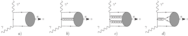
Figure 3: Twist-4 corrections to the pion transition form factor

Twist-four corrections to the form factor, by definition, correspond to the contributions of twist-four operators in the OPE of the time-ordered product of the two electromagnetic currents in Eq. (1). Such contributions are of order $1/Q^{4}$, but, as we will see later, are not the only ones that have to be taken into account to this accuracy: Twist counting does not coincide in the present case with the counting of powers of large momentum, so they should not be mixed.

Intuitively, twist-four effects can be thought of as due to quark transverse momentum (or virtuality) in the handbag diagram shown in Fig. 3a and quark-antiquark-gluon components in the pion wave function, Fig. 3b. These two contributions are related by exact QCD equations of motion Braun:1989iv ; hence they must be taken into account simultaneously. The corresponding calculation was done in Ref. Khodjamirian:1997tk . The result (for two virtual photons) can be written as

$$F_{\gamma^{*}\gamma^{*}\to\pi^{0}}(Q^{2},q^{2}) = \frac{\sqrt{2}f_{\pi}}{3}\Big{(}\int_{0}^{1}dx\frac{\phi_{\pi}(x)}{Q^{2}x+q^{2}\bar{x}}$$ (36)

$${}-\int_{0}^{1}dx\frac{\mathbb{F}_{\pi}(x)}{(Q^{2}x+q^{2}\bar{x})^{2}}\Big{)}.$$

and therefore

$$\frac{1}{\pi}\mathrm{Im}F_{\gamma^{\ast}\gamma^{\ast}\rightarrow\pi^{0}}(Q^{2},-s)=\frac{\sqrt{2}f_{\pi}}{3}\left[\frac{\phi_{\pi}(x)}{s+Q^{2}}-\frac{1}{Q^{2}}\frac{d\mathbb{F}_{\pi}(x)}{ds}\right]$$ (37)

with the usual substitution $x\equiv Q^{2}/(s+Q^{2})$. The first term on the r.h.s. of (36), (37) is the leading order twist-two contribution and ${\mathbb{F}_{\pi}(x)}$ is given in terms of the twist-4 pion DAs

$$\mathbb{F}_{\pi}(x,\mu)=\frac{1}{4}\phi_{4;\pi}(x)+\int_{0}^{\bar{x}}\!\!\!d\alpha_{1}\int_{0}^{x}\!\!\!d\alpha_{2}\left[\frac{1}{\alpha_{3}}\left(\frac{x\!-\!\bar{x}\!+\!\alpha_{1}\!-\!\alpha_{2}}{\alpha_{3}}\Phi_{4;\pi}(\underline{\alpha})-\widetilde{\Phi}_{4;\pi}(\underline{\alpha})\right)\right]_{\alpha_{3}=1-\alpha_{1}-\alpha_{2}}$$ (38)

where $\underline{\alpha}=\{\alpha_{1},\alpha_{2},\alpha_{3}\}$. The two-particle twist-4 DA $\phi_{4;\pi}(x)$ is defined by the light-cone expansion $y^{2}\to 0$ of the bilocal quark-antiquark operator Braun:1989iv ; Ball:1998je ; Ball:2006wn

$$\langle 0|\bar{q}(0)\gamma_{\mu}\gamma_{5}q(y)|\pi(p)\rangle=$$ (39)

$$= if_{\pi}p_{\mu}\!\int_{0}^{1}\!\!dx\,e^{-ixp\cdot y}\Big{[}\phi_{\pi}(x)+\frac{y^{2}}{16}\phi_{4;\pi}(x)\Big{]}+\ldots$$

and the three-particle DAs $\Phi_{4;\pi}(\underline{\alpha})$, $\widetilde{\Phi}_{4;\pi}(\underline{\alpha})$ correspond to the matrix elements

$$\langle 0|\bar{q}(0)\gamma_{\mu}\gamma_{5}gG_{\alpha\beta}(vn)q(un)|\pi(p)\rangle=$$

$$= p_{\mu}(p_{\alpha}n_{\beta}-p_{\beta}n_{\alpha})\,\frac{1}{pn}\,f_{\pi}\Phi_{4;\pi}(u,v;pn)+\dots,$$

$$\langle 0|\bar{q}(0)\gamma_{\mu}ig\widetilde{G}_{\alpha\beta}(vn)q(un)|\pi(p)\rangle=$$ (40)

$$= p_{\mu}(p_{\alpha}n_{\beta}-p_{\beta}n_{\alpha})\,\frac{1}{pn}\,f_{\pi}\widetilde{\Phi}_{4;\pi}(u,v:pn)+\dots,$$

with the shorthand notation

$${\cal F}(u,v;pn)=\int{\cal D}\underline{\alpha}\,e^{-ipn(u\alpha_{1}+v\alpha_{3})}{\cal F}(\underline{\alpha}).$$

The Wilson lines in the definitions of the nonlocal operators in (39), (40) are not shown for brevity. The integration measure is defined as ${\cal D}\underline{\alpha}=d\alpha_{1}d\alpha_{2}d\alpha_{3}\delta(1-\alpha_{1}-\alpha_{2}-\alpha_{3})$ and the dots denote contributions of other Lorentz structures that drop out and also terms of twist 5 and higher. Our notation follows Ref. Ball:2006wn .

Strictly speaking, there exist also twist-4 contributions from the wave function components containing two gluons or an extra quark-antiquark pair, Fig. 3c and Fig. 3d, but they are usually assumed to be small and neglected. The relevant argument is based on the specific property of four-particle twist-4 distributions: They do not allow for a factorization in terms of two-particle distributions and, say, quark or gluon condensate.

Higher-twist DAs can be studied using the conformal partial wave expansion, which is a generalization of the Gegenbauer polynomial expansion for the leading twist DAs Braun:1989iv . The contribution of the lowest conformal spin (asymptotic DAs) is

$$\mathbb{F}^{\rm as}_{\pi}(x,\mu) = \left(\frac{50}{3}+10\right)\delta_{\pi}^{2}(\mu)x^{2}(1-x)^{2}$$ (41)

$$= \frac{80}{3}\delta_{\pi}^{2}(\mu)x^{2}(1-x)^{2}$$

where the first and the second contribution in the parenthesis are the contributions of the two-particle and three-particle DAs in (38), respectively. We stress that these two contributions are related by exact equations of motion; taking into account e.g. the twist-4 correction to the handbag diagram and omitting contributions of three-particle DAs is inconsistent with QCD. One can show Braun:2007wv that the next-to-leading order conformal spin contributions to the relevant DAs do not contribute to $\mathbb{F}_{\pi}(x,\mu)$ so that this result is valid to NLO in the conformal expansion. The coupling $\delta_{\pi}^{2}$ is defined by the matrix element

$$\langle 0|\bar{q}g\widetilde{G}_{\mu\nu}\gamma^{\nu}q|\pi(p)\rangle=ip_{\mu}f_{\pi}\delta_{\pi}^{2}\,,$$

$$\delta_{\pi}^{2}(\mu)=\left(\frac{\alpha_{s}(\mu)}{\alpha_{s}(\mu_{0})}\right)^{32/(9\beta_{0})}\delta_{\pi}^{2}(\mu_{0})\,.$$ (42)

This parameter was estimated using the QCD sum rule approach in Novikov:1983jt (see also Bakulev:2002uc ):

$$\delta_{\pi}^{2}(\mu^{2}=1~{}\mbox{GeV}^{2})\simeq 0.2~{}\mbox{GeV}^{2}\,.$$ (43)

III.4 Twist-six corrections

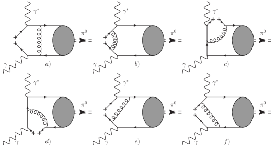
Figure 4: Factorizable twist-6 corrections to the $F_{\gamma^{*}\gamma\to\pi^{0}}(Q^{2})$ form factor.

The calculation of twist-six corrections to the transition form factor presents a new result of this work. To explain why such corrections may be important, consider an example of the Feynman diagram shown in Fig. 4a. The broken quark line with crosses stands for the quark condensate. If both photon virtualities are large, this diagram contributes to the OPE of the product of the two electromagnetic currents (the so-called cat-ears contribution) which involves the twist-6 four-quark pion DA in the factorization approximation: One quark-antiquark pair is put in the condensate and the other one forms a twist-3 chiral-odd quark-antiquark DA. Explicit calculation gives (cf. Khodjamirian:1997tk )

$$F^{\rm Fig.\,4a}_{\gamma^{*}\gamma^{*}\to\pi^{0}}(Q^{2},q^{2})=\frac{\sqrt{2}f_{\pi}}{3}\,\frac{32\pi\alpha_{s}\langle\bar{q}q\rangle^{2}}{9f_{\pi}^{2}q^{2}Q^{2}}\int_{0}^{1}\frac{dx\,\phi^{p}_{3;\pi}(x)}{xQ^{2}+\bar{x}q^{2}},$$ (44)

where Braun:1989iv ; Ball:1998je ; Ball:2006wn

$$\langle 0|\bar{q}(0)i\gamma_{5}q(\alpha n)|\pi(p)\rangle=\frac{f_{\pi}m_{\pi}^{2}}{m_{u}+m_{d}}\,\int_{0}^{1}dx\,e^{-ix\alpha pn}\,\phi^{p}_{3;\pi}(x)\,.$$ (45)

The DA $\phi^{p}_{3;\pi}(x)$ is related to the contribution of three-particle (quark-antiquark-gluon) Fock state by equations of motion Braun:1989iv . If the contributions of the twist-3 three-particle DA are neglected, $\phi^{p}_{3;\pi}(x)=1$ must be taken Braun:1989iv ; Ball:1998je ; Ball:2006wn . In Eq. (44) we used the Gell-Mann-Oakes-Renner relation $(m_{u}+m_{d})(\langle\bar{u}u\rangle+\langle\bar{d}d\rangle)=-f_{\pi}^{2}m_{\pi}^{2}$ which is exact in the chiral limit.

For the case of two equal large virtualities $q^{2}=Q^{2}$ this contribution is of order $\langle\bar{q}q\rangle^{2}/Q^{6}$, so it is suppressed by two extra powers of $1/Q^{2}$ compared to the leading term, as expected from dimension (twist) counting. On the other hand, the real photon limit $q^{2}\to 0$ of (44) cannot be taken in a straightforward way since the pole at $q^{2}=0$ is clearly unphysical. This singularity appears, obviously, because the quark interacting with the soft photon comes close to the mass shell. Thus the distance it travels becomes large and the OPE cannot be applied. In the full theory, this singularity will be tamed by nonperturbative corrections corresponding to photon emission from large distances, Fig. 1b. In the simplest, vector meson dominance (VDM) approximation (in the LCSR method in addition the continuum contribution is taken into account) nonperturbative corrections amount to a replacement $1/q^{2}\to 1/(m_{\rho}^{2}+q^{2})$ so that for $q^{2}\to 0$ the singular factor $1/q^{2}$ is replaced by $1/m_{\rho}^{2}$. One obtains

$$F^{\rm Fig.\,4a}_{\gamma^{*}\gamma\to\pi^{0}}(Q^{2})\simeq\frac{\sqrt{2}f_{\pi}}{3}\,\frac{32\pi\alpha_{s}\langle\bar{q}q\rangle^{2}}{9f_{\pi}^{2}m_{\rho}^{2}Q^{4}}\int_{0}^{1}\!dx\,\frac{\phi^{p}_{3;\pi}(x)}{x+\bar{x}m_{\rho}^{2}/Q^{2}}\,.$$ (46)

Note that this is a $1/Q^{4}$ correction to the form factor, not $1/Q^{6}$ as for equal virtualities. The factor $1/m_{\rho}^{2}$ can be identified with the magnetic susceptibility of the quark condensate (in the VDM approximation) Ioffe:1983ju ; Belyaev:1984ic ; Balitsky:1985aq ; Balitsky:1989ry ; Ball:2002ps

$$\chi\simeq\frac{2}{m_{\rho}^{2}}\simeq 3.3~{}\mbox{GeV}^{-2}.$$ (47)

which enters the definition of the leading twist DA of a real photon Balitsky:1989ry ; Ball:2002ps so that this contribution can be rewritten as a convolution of photon and pion DAs with the coefficient function corresponding to a hard gluon exchange, cf. Fig. 1b. The direct calculation of this contribution gives

$$F^{\rm Fig.\,1b}_{\gamma^{*}\gamma\to\pi^{0}}(Q^{2}) = \frac{\sqrt{2}f_{\pi}}{3}\,\frac{16\pi\alpha_{s}\chi\langle\bar{q}q\rangle^{2}}{9f_{\pi}^{2}Q^{4}}$$ (48)

$${}\times\int_{0}^{1}\!dx\,\frac{\phi^{p}_{3;\pi}(x)}{x}\int_{0}^{1}\!dy\,\frac{\phi_{\gamma}(y)}{\bar{y}^{2}}\,,$$

where $\phi_{\gamma}(y)\simeq 6y(1-y)$ is the leading-twist photon DA Balitsky:1989ry ; Ball:2002ps . The integrals over the quark momentum fractions in (48) are both logarithmically divergent at the end-points $x\to 0$, $y\to 1$, which signals that there is an overlap with the soft region, Fig. 1c.

Another twist-6 contribution comes from the diagram in Fig. 4b

$$F^{\rm Fig.\,4b}_{\gamma^{*}\gamma^{*}\to\pi^{0}}(Q^{2},q^{2})=\frac{\sqrt{2}f_{\pi}}{3}\frac{64\pi\alpha_{s}\langle\bar{q}q\rangle^{2}}{27f_{\pi}^{2}}\!\int_{0}^{1}\!\!\frac{dx\,\phi^{\sigma}_{3;\pi}(x)}{(xQ^{2}\!+\!\bar{x}q^{2})^{3}},$$ (49)

where the DA $\phi^{\sigma}_{3;\pi}(x)$ is defined as

$$\langle 0|\bar{q}(0)\sigma_{\mu\nu}\gamma_{5}q(\alpha n)|\pi(p)\rangle = \frac{i}{6}(p_{\mu}x_{\nu}-p_{\nu}x_{\mu})\frac{f_{\pi}m_{\pi}^{2}}{m_{u}+m_{d}}$$ (50)

$$\times \!\int_{0}^{1}\!dx\,e^{-ix\alpha pn}\,\phi^{\sigma}_{3;\pi}(x)\,.$$

In the considered approximation (neglecting the quark-antiquark-gluon DAs) the asymptotic form $\phi^{\sigma}_{3;\pi}(x)\,=\,6x(1-x)$ must be taken Braun:1989iv ; Ball:1998je ; Ball:2006wn . Note that this contribution is also of the order of $1/Q^{4}$ and not $1/Q^{6}$ as suggested by the naive power counting, since the limit $q^{2}\to 0$ leads to a quadratic divergence $\int dx/x^{2}$ at small momentum fractions. As above, this divergence is regulated in the LCSR approach by correcting the spectral density to include the $\rho(\omega)$-resonance and the continuum.

Next, the diagrams in Figs. 4c,d can be calculated using the light-cone expansion of the quark propagator in a background gluon field Balitsky:1987bk and picking up terms containing covariant derivatives of the gluon field strength $D^{\mu}G_{\mu\nu}$. These can be reduced to a quark-antiquark pair via equations of motion. We have checked that there are no terms with additional derivatives compared to the expression given in Balitsky:1987bk contributing at the required twist 6 level. A straightforward albeit rather lengthy calculation gives

$$F^{\rm Fig.\,4c,d}_{\gamma^{*}\gamma^{*}\to\pi^{0}}(Q^{2},q^{2}) = -\dfrac{\sqrt{2}f_{\pi}}{3}\frac{16\pi\alpha_{s}\langle\bar{q}q\rangle^{2}}{27f_{\pi}^{2}}\int_{0}^{1}dv(v-\bar{v})v\int_{0}^{1}du\dfrac{u-v}{\bar{u}}\phi^{\sigma}_{3;\pi}(u)$$ (51)

$$\times \left\{\dfrac{1}{[uvq^{2}+(1-uv)Q^{2}]^{3}}+\dfrac{1}{[(1-uv)q^{2}+uvQ^{2}]^{3}}\right\},$$

where it was used that to our accuracy

$$\frac{x}{2}\left(\phi^{p}_{3;\pi}(x)+\frac{1}{6}\frac{d\phi^{\sigma}_{3;\pi}(x)}{dx}\right) = \frac{1}{6}\phi^{\sigma}_{3;\pi}(x)$$

$$\frac{\bar{x}}{2}\left(\phi^{p}_{3;\pi}(x)-\frac{1}{6}\frac{d\phi^{\sigma}_{3;\pi}(x)}{dx}\right) = \frac{1}{6}\phi^{\sigma}_{3;\pi}(x).$$ (52)

Finally, the diagrams in Figs. 4e,f vanish. This is in difference to the similar calculation for the pion electromagnetic form factor in Ref. Braun:1999uj where only these diagrams contributed.

III.5 The complete sum rule

Collecting all contributions, we present here the complete light-cone sum rule with twist-6 accuracy, which will be used in numerical analysis in the next section.

The sum rule for the $\pi^{0}\gamma^{*}\gamma$ form factor can be written in terms of the full QCD spectral density $\rho(Q^{2}\!,s)$ as

$$F_{\gamma^{\ast}\gamma\to\pi^{0}}(Q^{2}) = \frac{\sqrt{2}f_{\pi}}{3}\Big{[}\int_{s_{0}}^{\infty}\frac{ds}{s}\rho(Q^{2},s)$$ (53)

$$+\frac{1}{m_{\rho}^{2}}\int_{0}^{s_{0}}\!\!ds\,\rho(Q^{2}\!,s)e^{(m_{\rho}^{2}-s)/M^{2}}\Big{]}$$

$$\equiv F^{\rm hard}_{\gamma^{\ast}\gamma\to\pi^{0}}(Q^{2})+F^{\rm soft}_{\gamma^{\ast}\gamma\to\pi^{0}}(Q^{2})\,.$$

Here we define the “hard” and the “soft” contributions as coming from large $s>s_{0}$ and small $s<s_{0}$ invariant masses in the dispersion integral, respectively. Note that the hard part is model-independent whereas the soft part is obtained under the assumption that the contribution of small invariant masses can be represented by a single narrow resonance. The continuum threshold $s_{0}$ can be viewed as the separation scale between hard and soft contributions; the dependence on $s_{0}$ has to cancel in the sum.

The QCD spectral density, in turn, can be calculated as a sum of contributions of different twists, $t$=2,4,6

$$\rho(Q^{2}\!,s)=\rho^{(2)}(Q^{2}\!,s)+\rho^{(4)}(Q^{2}\!,s)+\rho^{(6)}(Q^{2}\!,s)+\ldots$$ (54)

The leading-twist spectral density to the NLO accuracy is given by

$$\rho^{(2)}(Q^{2},s) = \frac{x}{Q^{2}}\sum_{n=0.2\ldots}^{\infty}a_{n}(\mu)\Bigg{\{}\varphi_{n}(x)+\frac{C_{F}\alpha_{s}(\mu)}{4\pi}$$ (55)

$$\times \Bigg{[}R_{n}(Q^{2},s)\varphi_{n}(x)+\tilde{\gamma}_{n}^{0}\sum_{k=0,1..}^{n}H_{n}^{k}\varphi_{k}(x)$$

$$+2\sum_{k=0,2..}^{n}G_{n}^{k}\varphi_{k}(x)-3\tilde{\gamma}_{n}^{0}\bar{x}\Bigg{]}\Bigg{\}},$$

where

$$R_{n}(Q^{2},s) = -3\Big{[}1+2(\psi(2)-\psi(2+n)\Big{]}$$ (56)

$${}+\frac{\pi^{2}}{3}-\ln^{2}\left(\frac{\bar{x}}{x}\right)-\tilde{\gamma}_{n}^{(0)}\ln\left(\frac{s}{\mu^{2}}\right).$$

The integrals corresponding to the “hard” part, $s>s_{0}$, in Eq. (53) can be taken analytically. The corresponding expression in Eq. (E.17) in Bakulev:2002uc contains a misprint: the term $-3\ln^{2}(s_{0}/u)$ has to be replaced by $-3\ln(s_{0}/u)$.

The twist-4 spectral density is equal to

$$\rho^{(4)}(Q^{2},s)=\frac{160}{3Q^{4}}\delta_{\pi}^{2}(\mu)x^{3}\bar{x}(1-2x)\,.$$ (57)

Finally, the twist-6 contribution can be written as:

$$\rho^{(6)}(Q^{2}\!,s) = 8\pi C_{F}\alpha_{s}(\mu)\dfrac{\langle\bar{q}q\rangle^{2}}{N_{c}f_{\pi}^{2}}\dfrac{x^{2}}{Q^{6}}\Bigg{[}2x\log x+2x\log\bar{x}$$ (58)

$${}-x+2\delta(\bar{x})-\frac{1}{\bar{x}}+\delta(\bar{x})\int_{0}^{1}\frac{dx^{\prime}}{\bar{x}^{\prime}}\Bigg{]}.$$

Note that the last two terms combine to a “plus” distribution, $1/[1-x]_{+}$. In all expressions (55)–(58) $x\equiv Q^{2}/(Q^{2}+s)$.

We want to emphasize that the twist-6 contribution is not suppressed compared to the twist-4 one by an extra power of $Q^{2}$, and the same is true for all higher-twist corrections. The twist expansion in LCSRs goes in powers of $\Lambda^{2}_{\rm QCD}/s_{0}$, $\Lambda^{2}_{\rm QCD}/M^{2}$ where $\Lambda^{2}_{\rm QCD}$ is a generic dimensionful parameter that characterizes the size of higher-twist matrix elements.

IV Numerical Analysis

IV.1 The parameters

All numerical results in this work are obtained using the two-loop running QCD coupling with $\Lambda_{\rm QCD}^{(4)}=326$ MeV and $n_{f}=4$ active flavors. Unless stated otherwise, all nonperturbative parameters and models of the pion DA refer to the renormalization scale $\mu_{0}=1$ GeV; $\alpha_{s}(\mu_{0})=0.494$.

A natural factorization and renormalization scale $\mu$ in the calculation of the $\pi^{0}\gamma^{*}\gamma^{*}$ form factor with two large virtualities is given by the virtuality of the quark propagator $\mu^{2}\sim xQ^{2}+\bar{x}q^{2}$ and depends on the quark momentum fraction. If $q^{2}\to 0$, in the LCSR framework the relevant factorization scale becomes $\mu^{2}\sim xQ^{2}+\bar{x}M^{2}$ or $\mu^{2}\sim xQ^{2}+\bar{x}s_{0}$ for large values of the Borel parameter, see e.g. Braun:1999uj . Note that in the first integral in (53) the quark virtuality is never large, of order $Q^{2}$: The restriction $s<s_{0}$ translates to $\bar{x}<s_{0}/(s_{0}+Q^{2})$ and hence $\mu^{2}\simeq 2s_{0}$ as $Q^{2}\to\infty$, in agreement with the interpretation of this term as the “soft” contribution. Numerical calculations with the $x$-dependent factorization scale are rather slow so in this work we use a fixed scale, replacing $x$ by the constant $\langle x\rangle$ which is varied within a certain range:

$$\mu^{2}=\langle x\rangle\,Q^{2}+\langle\bar{x}\rangle\,s_{0}\,,\qquad 1/4<\langle x\rangle<3/4\,.$$ (59)

The choice of the Borel parameter in LCSRs is discussed in Ali:1993vd ; Ball:1997rj . The subtlety is that the twist expansion in LCSRs goes in powers of $1/(xM^{2})$ rather than $1/M^{2}$ in the classical SVZ approach. Hence one has to use somewhat larger values of $M^{2}$ compared to the QCD sum rules for two-point correlation functions in order to ensure the same hierarchy of contributions. We choose as the “working window”

$$1<M^{2}<2~{}\text{GeV}^{2}$$ (60)

and $M^{2}=1.5$ GeV² as the default value in our calculations.

We use the standard value $s_{0}=1.5$ GeV² for the continuum threshold as the central value, and the range

$$1.3<s_{0}<1.7~{}\text{GeV}^{2}$$ (61)

in the error estimates. We did not attempt to consider corrections due to the finite width of the $\rho,\omega$ resonances. The estimates in Ref. Mikhailov:2009kf suggest that such corrections may result in the enhancement of the form factor by 2-4% in the small-to-mediate $Q^{2}$ region where the resonance part dominates. We believe that such uncertainties are effectively covered by our (conservative) choice of the continuum threshold.

Finally, we use the values $\delta_{\pi}^{2}=0.2\pm 0.4$ GeV² and $\langle\bar{q}q\rangle=-(240\pm 10~{}\text{MeV})^{3}$ (at the scale 1 GeV) for the normalization parameter for twist-4 DAs (43) and the quark condensate, respectively.

IV.2 Testing simple models

We start our analysis with the comparison of the LCSR predictions for the $\pi^{0}\gamma^{*}\gamma$ form factor for three simple models of the pion DA that are often quoted in the literature:

$$\phi_{\pi}^{\rm as}(x) = 6x(1-x)\,,$$

$$\phi_{\pi}^{\rm hol}(x) = \frac{8}{\pi}\sqrt{x(1-x)}\,,$$

$$\phi_{\pi}^{\rm flat}(x) = 1\,.$$ (62)

The asymptotic $\phi_{\pi}^{\rm as}(x)$ and flat $\phi_{\pi}^{\rm flat}(x)$ DAs have already been discussed above; the “holographic” model $\phi_{\pi}^{\rm hol}(x)$ is inspired by the AdS/QCD correspondence Brodsky:2007hb (see, however, Grigoryan:2008up ).

Apart from the general interest, considering these models allows one to test the applicability of the Gegenbauer expansion. To this end, consider the approximations to $\phi_{\pi}^{\rm flat}(x)$, $\phi_{\pi}^{\rm hol}(x)$ by the truncated series at order $n$:

$$\phi_{\pi}^{\rm flat(\rm hol),(n)}(x) = \sum_{k=0,2,\ldots}^{n}a_{k}^{\rm flat(\rm hol)}\varphi_{k}(x)\,,$$ (63)

where

$$a_{k}^{\rm hol}=\frac{2n+3}{3\pi}\left(\frac{\Gamma[(n+1)/2]}{\Gamma[(n+4)/2]}\right)^{2}$$ (64)

and $a_{k}^{\rm flat}$ are given in Eq. (15).

The expressions collected in Sect. 3 and App. A,B allow us to construct the sum rules using up to seven terms $k=0,2,\ldots,12$ corresponding to the $n=12$ truncation. The resulting DAs $\phi_{\pi}^{\rm flat,(n=12)}(x)$, $\phi_{\pi}^{\rm hol,(n=12)}(x)$ are compared with the exact ones, $\phi_{\pi}^{\rm flat}(x)$, $\phi_{\pi}^{\rm hol}(x)$, in Fig. 5. Note that the $n=12$ approximation is very good for the “holographic” DA, whereas for the “flat” one the convergence is slow and there are large oscillations.

Figure 5: The $n=12$ truncations (63) of the pion DAs $\phi_{\pi}^{\rm hol}(x)$ and $\phi_{\pi}^{\rm flat}(x)$ compared to the exact expressions.

Next, we use the three DAs in Eq. (62) (the last two ones truncated at order $n=12$) to calculate the $\pi^{0}\gamma^{*}\gamma$ form factor. The results are shown in Fig. 6.

Figure 6: The pion transition form factor for the “flat” (solid red line), “holographic” (dashed blue line) and “asymptotic” (dash-dotted blue line) models for the pion DA, cf. Eq. (62). The experimental data are from BABAR (full circles) and Gronberg:1997fj (open triangles).

One sees that both the asymptotic and holographic models fail to describe the BaBar data BABAR . The flat DA fares better for the largest $Q^{2}$ values, but is considerably above the experiment at intermediate $Q^{2}\sim 5-15$ GeV². In order to understand this behavior, we compare in Fig. 7 the predictions for three different truncations of the flat DA: $\phi_{\pi}^{\rm flat,(n=12)}(x)$, $\phi_{\pi}^{\rm flat,(n=8)}(x)$ and $\phi_{\pi}^{\rm flat,(n=4)}(x)$.

Figure 7: The pion transition form factor for three different approximations for the “flat” DA: $n=12$ (solid red line), $n=8$ (dashed blue line), and $n=4$ (dash-dotted). The experimental data are from BABAR (full circles) and Gronberg:1997fj (open triangles).

We observe that all three calculations are very close to each other for $Q^{2}\leq 18$ GeV² so that in this region contributions of Gegenbauer polynomials starting with $n=6-8$ play no role. This conclusion is in agreement with our discussion of the MR model in Sect. 2 and also supports the usual procedure of modelling the pion DA by the asymptotic expression and contributions of first two Gegenbauer polynomials in applications to $B$-decays and pion electromagnetic form factor, e.g. Khodjamirian:1997tk ; Schmedding:1999ap ; Bakulev:2001pa ; Bakulev:2002uc ; Bakulev:2003cs ; Agaev:2005rc ; Mikhailov:2009kf . We also see that contributions of the Gegenbauer polynomials $n=6\,,8$ become significant for the momentum transfers $Q^{2}>18\,{\rm GeV}^{2}$. In the region $Q^{2}>30\,{\rm GeV}^{2}$ higher-order polynomials should be included into analysis as well, but the accuracy of the existing experimental data is not sufficient to draw definite conclusions.

In other words, the differences between the predictions of asymptotic, holographic and flat DAs in Fig. 6 for $Q^{2}<20~{}{\rm GeV}^{2}$ are mostly due to the different values of the coefficients $a_{2}$ and $a_{4}$, with $a_{6}$ also playing some role. This leaves us with $2-3$ parameters that can be tuned to attempt a better description of the BaBar data, the task that we address now.

IV.3 Confronting the BaBar data

The extraction of the pion DA with meaningful error estimates requires a global fit to the pion transition and electromagnetic form factor, weak $B(D)\to\pi\ell\nu$ decays and the couplings $g_{\pi NN},g_{BB^{*}\pi}$ etc. using a Monte Carlo scan of the space of all available parameters, which goes beyond the tasks of this work. Fitting of the BaBar data is not attempted. Instead, we present results for three sample models that describe the $\pi^{0}\gamma^{*}\gamma$ form factor sufficiently well and discuss their general features.

The three models that we consider below are shown in Fig. 8 (at the scale 1 GeV) and the corresponding Gegenbauer coefficients are collected in Table 2.

The first model

$$\phi_{\pi}^{\rm I}(x)=1-(7/18-0.13)\varphi_{2}(x)$$ (65)

is nothing but the flat DA with the reduced second Gegenbauer coefficient, $a^{\rm flat}_{2}\to 0.130$.

Figure 8: Model I, (red solid curve), model II (blue dashed curve) and model III (black dash-dotted curve) of the pion DA at the scale 1 GeV. The asymptotic pion DA is shown by green dots for comparison.

Model	scale	$a_{2}$	$a_{4}$	$a_{6}$	$a_{8}$	$a_{10}$	$a_{12}$
I	$\mu=1$ GeV	0.130	0.244	0.179	0.141	0.116	0.099
	$\mu=2$ GeV	0.089	0.148	0.097	0.070	0.054	0.044
II	$\mu=1$ GeV	0.140	0.230	0.180	0.05	0.0	0.0
	$\mu=2$ GeV	0.096	0.140	0.098	0.024	-0.001	$<10^{-3}$
III	$\mu=1$ GeV	0.160	0.220	0.080	0.0	0.0	0.0
	$\mu=2$ GeV	0.110	0.133	0.043	-0.001	$<10^{-3}$	$<10^{-3}$

Table 2: Gegenbauer coefficients of three sample models of pion DA that are consistent with BaBar measurements BABAR of the transition form factor, cf. Fig. 9.

It has a long “tail” of higher-order Gegenbauer polynomials. From the previous discussion we expect that this “tail” actually gives no contribution in the $Q^{2}$ range of interest. In order to check that this is indeed the case, we consider the second model in which the higher-order coefficients $a_{10},a_{12}$ are put to zero at the reference scale 1 GeV, and we keep a small $a_{8}$ to avoid an oscillating behavior at $x\sim 1/2$. Note that nonzero values of the coefficients $a_{10},a_{12}$ (and all higher) are generated at higher scales, but this mixing is numerically insignificant. Finally, the third model is chosen to explore the sensitivity of the predictions to particular values of $a_{2},\,a_{4}$ and $a_{6}$, and to see whether they are correlated.

The calculations using these models are compared with the available experimental data in Fig. 9. The results are shown by thick solid curves: The line thickness shows the uncertainty and is calculated as a square root of the sum of squares of the error bars on the LCSR predictions due to variation of the parameters within the limits specified in Sect. IV.A. These include the factorization scale dependence, dependence on the Borel parameter $M^{2}$ and the continuum threshold $s_{0}$, and on higher-twist parameters $\delta_{\pi}^{2}$ and $\langle\bar{q}q\rangle$.

Figure 9: The pion transition form factor for the three models of the pion DA specified in the text. The experimental data are from BABAR (full circles) and Gronberg:1997fj (open triangles).

The distinctive feature of all three models is the large value of the fourth Gegenbauer moment, $a_{4}$, which is necessary in order to accommodate the observed rise of the scaled form factor in the $Q^{2}=5-20$ GeV² range. It is not possible to trade the large value of $a_{4}$ for the increased $a_{2}$ or $a_{6}$, although of course there is some correlation.

Our value of $a_{2}\sim 0.13-0.16$ at 1 GeV is at the low end of the existing estimates, cf. Table. 1, and in particular it is lower compared to the earlier LCSR analysis of the transition form factor in Refs. Bakulev:2002uc ; Mikhailov:2009kf ; Agaev:2005rc . The main reason for this difference is that the Borel parameter in Bakulev:2002uc ; Mikhailov:2009kf is fixed at an ad hoc value $M^{2}=0.7\,{\rm GeV}^{2}$, whereas in the present analysis we allow its variation in the $1-2$ GeV² range. For the specific choice $a_{2}(\mu_{\rm SY})=0.14$, $a_{4}(\mu_{\rm SY})=-0.09$, $\mu_{\rm SY}\simeq 2.4$ GeV, advocated in Bakulev:2002uc ; Mikhailov:2009kf , the result for the form factor at $Q^{2}=5$ GeV² is increased by $\sim 11\%$ if $M^{2}$ is changed from 0.7 to 1.5 GeV². Another reason is that in Bakulev:2002uc ; Mikhailov:2009kf ; Agaev:2005rc the twist-6 correction is not included. The size of this correction depends strongly on the Borel parameter. For our choice $M^{2}\sim 1.5\pm 0.5$ GeV² the twist-6 term proves to be small: factor three smaller that the twist-4 correction (see below), which is gratifying as it signals convergence of the OPE. In contrast, at $M^{2}=0.7$ GeV² the twist-6 correction is almost of the same size as twist 4 and has opposite sign. Hence it must be included. In both cases (increasing the Borel parameter and/or including the twist-6 correction) the net effect is the increase of the form factor by 5-10% in the CLEO range which has to be compensated by a smaller value of the second Gegenbauer moment.

The error band indicated by thickness of the curves in Fig. 9 has to be taken with caution. A weak scale dependence of our results is largely due to strong cancellations of the NLO radiative corrections between the contributions of the asymptotic DA and higher Gegenbauer polynomials and may not be representative for the size of NNLO corrections which are only known in the $\overline{\mbox{\rm CS}}$ factorization scheme, see Melic:2002ij for a detailed discussion of the related ambiguities. Also the uncertainty in the twist-4 contribution is not reduced to the $\delta_{\pi}^{2}$ parameter: Using an alternative, renormalon model Braun:2004bu of the twist-4 pion DA generally produces somewhat larger corrections. We have checked that the difference is not very significant, however, and does not affect any of our conclusions. Hence we do not show the corresponding results.

The “hard” and “soft” contributions to the $\pi^{0}\gamma^{*}\gamma$ form factor as defined in Eq. (53) are shown separately for model I (solid curves) and model III (dash-dotted curves) in Fig. 10.

Figure 10: Contributions to the $\pi^{0}\gamma^{*}\gamma$ form factor from large (“hard”) and small (“soft”) invariant masses in the dispersion representation, cf. Eq. (53), for model I (solid curves) and model III (dash-dotted curves). The experimental data are from BABAR (full circles) and Gronberg:1997fj (open triangles).

Asymptotically, for $Q^{2}\to\infty$, the soft contribution is power-suppressed compared to the hard one, $\sim s_{0}/Q^{2}$. This suppression sets in for very large values of $Q^{2}$, however, especially if the pion DA is enhanced close to the end points. E.g. for our model III the soft contribution still accounts for ca. 25% of the form factor at $Q^{2}=30$ GeV² (for the separation scale $s_{0}=1.5$ GeV²). This means that a purely perturbative leading twist QCD calculation of the transition form factor for one real photon in collinear factorization should not be expected to have high accuracy. A lattice calculation of the transition $\pi\rho\gamma^{*}$ form factor at $Q^{2}\sim 2-5$ GeV² would help to estimate the contribution of the resonance region more reliably.

Finally, in Fig. 11 we show the higher-twist contributions. The twist-4 correction is negative and the twist-6 one is positive. It turns out that the twist-6 contribution depends rather strongly on the Borel parameter. It is suppressed in the $Q^{2}$ region of interest relative to the twist-4 term for our choice $M^{2}=1.5\,{\rm{GeV}}^{2}$, but increases rapidly for smaller $M^{2}$. For example, for $M^{2}=0.7\,{\rm{GeV}}^{2}$ used in Bakulev:2002uc ; Mikhailov:2009kf , the twist-6 correction is $\sim 0.6$ of the twist-4 term at $Q^{2}=1\,{\rm{GeV}}^{2}$, becomes equal (with opposite sign) at $Q^{2}\simeq 14\,{\rm{GeV}}^{2}$ and overshoots twist-4 for larger $Q^{2}$ (because it contains a logarithmic $\sim\ln Q^{2}$ enhancement).

Figure 11: Higher twist contributions to the $\pi^{0}\gamma^{*}\gamma$ form factor for the values of the Borel parameter $M^{2}=1.5$ (solid curves) and $M^{2}=0.7$ GeV² (dashed curves).

IV.4 Other processes

The pion DA is a universal function and, if extracted from one reaction, should, in general, describe all exclusive or semi-inclusive processes that involve a pion in the initial and/or final states. The most prominent of them are the pion electromagnetic form factor and the weak semileptonic decay rate $B\to\pi\ell\nu_{\ell}$. Without going in detail, we present here the corresponding LCSR calculations using the pion DA models as specified above.

The LCSRs for the pion electromagnetic form factor were derived in Refs. Halperin ; Braun:1999uj ; Bijnens:2002mg and later explored also in Agaev:2005gu ; Agaev:2008 . These sum rules are known to the same accuracy as for the transition form factor, i.e. including the NLO perturbative contribution, twist-4 and twist-6 corrections. Explicit expressions can be found in Bijnens:2002mg .

The results are shown in Fig. 12 in comparison with the experimental data Bebek ; Fpi . For this plot we have chosen $M^{2}=1.5$ GeV², $s_{0}^{\pi}=0.8$ GeV² and the factorization scale $\mu=(1/2)(Q^{2}+s_{0})$ as representative values; the three curves correspond to the models of the pion DA in Fig. 8.

Figure 12: Electromagnetic pion form factor for the three models of pion DA described in the text. Identification of the curves follows Fig. 8. The experimental data are from Bebek (blue squares) and Fpi (red circles).

The agreement is very good. Note that the oscillations at small $Q^{2}$ in model I are an artifact of the truncation of the Gegenbauer expansion. They can be removed, e.g. by reducing $a^{\rm flat}_{12}=0.099\to 0.04$ which has the effect of smoothening the DA, especially in the central region.

It has to be mentioned that the pion electromagnetic form factor is much more affected by soft contributions compared to the transition form factor and hence is also more model dependent. In particular the Borel parameter dependence is much stronger, see Fig. 13, where the calculations using $M^{2}=1$ and $M^{2}=2$ GeV² are shown by dashed curves for comparison.

Figure 13: Electromagnetic pion form factor for model I (with reduced $a_{12}=0.099\to 0.04$). The solid curve, upper dashed curve and lower dashed curve are calculated using the Borel parameter $M^{2}=1.5$, $M^{2}=2$ and $M^{2}=1$ GeV², respectively. The experimental data are from Bebek (blue squares) and Fpi (red circles).

The weak decay $B\to\pi\ell\nu_{\ell}$ has received a lot of attention as one of primary sources of information on the weak mixing angle $|V_{ub}|$ in the Standard Model. The differential decay width $dB/dq^{2}$, where $q^{2}$ is the invariant mass of the leptons, is given by the square of the $B\to\pi$ form factor, modulo relevant CKM angles and kinematic factors

$$\dfrac{dB}{dq^{2}}(B\to\pi^{-}e^{+}\nu_{e})=\dfrac{G_{F}^{2}|V_{ub}|^{2}}{192\pi^{3}m_{B}^{3}}\tau_{B}\,\lambda^{3/2}(q^{2})\,|f_{B\pi}^{+}(q^{2})|^{2}\,.$$ (66)

In this equation $\lambda(q^{2})=(m_{B}^{2}+m_{\pi}^{2}-q^{2})^{2}-4m_{B}^{2}m_{\pi}^{2}$ and $\tau_{B}$ is the mean life time of the B-meson. Below we use $|V_{ub}|=3.6\cdot 10^{-3}$ to fix the overall normalization.

LCSRs enable one to calculate the form factor up to $q^{2}=14$ GeV², and a two parameter BCL Bourrely:2008za fit is then used to extrapolate the calculation to the whole kinematic region $0\leq q^{2}\leq 26.4$ GeV². The latest and most advanced LCSR calculations of this form factor Duplancic:2008ix ; Ball:2004ye include NLO corrections in leading twist and also for a part of the twist-3 contributions. Twist-4 corrections are taken into account in the leading order. In the calculations presented in Fig. 14 we use the central values of the sum rule parameters from Ref. Duplancic:2008ix .

Figure 14: The differential $\pi^{-}e^{+}\nu_{e}$ decay width. Experimental data are taken from :2010zd . A 2-parameter BCL-fit Bourrely:2008za is applied to the sum rule calculation to extrapolate it to the whole $q^{2}$ range. For normalization we assume $|V_{ub}|=3.6\cdot 10^{-3}$. The identification of the curves follows Fig. 8, see also text.

All our models of pion DA describe the data :2010zd reasonably well and are nearly indistinguishable in the $q^{2}<14$ GeV² range where the direct sum rule calculation is applicable. The calculation using “conventional” pion DA with $a_{2}=0.17$ and $a_{4}=0.06$ (at 1 GeV) Duplancic:2008ix is shown by green dots for comparison. We conclude that the $B\to\pi$ form factor is not very sensitive to the higher Gegenbauer moments beyond $a_{2}$; a low value $a_{2}<0.2$ (at 1 GeV) is preferred.

The value of the pion DA in the middle point in all our models is close to the asymptotic value $\phi_{\pi}(x=1/2)=1.5$. This number is within the range in Eq. (13) and somewhat larger than it was assumed in the LCSR calculations of pion-hadron couplings Braun:1988qv ; Belyaev:1994zk ; Khodjamirian:1999hb ; Aliev:1999ce ; Aliev:2006xr ; Aliev:2009kg . The larger value is in fact welcome and can reduce the well-known $\sim 30\%$ discrepancy of the sum rule calculation Belyaev:1994zk ; Khodjamirian:1999hb of $g_{D^{*}D\pi}$ with the experiment.

V Summary and Conclusions

The recent BaBar measurement BABAR of the pion transition form factor provided one with the most direct evidence so far that the pion distribution amplitude deviates considerably from its asymptotic form. This result has to be considered as a success of an early QCD prediction Chernyak:1981zz of a broad pion DA at a low scale, but it also created a lot of excitement because a significant scaling violation at $Q^{2}>5-10$ GeV² came out unexpected.

The main lesson to be learnt from the BaBar data is that attempts to describe the transition form factor with one real photon entirely in the framework of perturbative QCD are futile; nonperturbative soft corrections must be taken into account.

We have adopted the LCSR approach Balitsky:1989ry ; Braun:1988qv ; Chernyak:1990ag which has the advantage that it is applicable to a broad class of reactions and has been thoroughly tested. In this work we go beyond the existing analysis Khodjamirian:1997tk ; Schmedding:1999ap ; Bakulev:2001pa ; Bakulev:2002uc ; Bakulev:2003cs ; Agaev:2005rc ; Mikhailov:2009kf in two aspects. First, we calculate a new, twist-six contribution to LCSRs which proves to be sizeable. Second, we extend the existing formalism to allow for the contributions of higher-order Gegenbauer polynomials, which allows one to consider DAs of arbitrary shape and also address the question of convergence of the Gegenbauer expansion which generated some confusion.

We find that a significant rise of the scaled form factor $Q^{2}F_{\pi^{0}\gamma^{*}\gamma}(Q^{2})$ in the $Q^{2}=5-20$ GeV² range observed by the BaBar collaboration BABAR can be explained by a large value of the fourth Gegenbauer moment

$$a_{4}>a_{2}$$

in the pion DA, leading to models of the type shown in Fig. 8 which are not far from the asymptotic distribution in the central region but have enhancements close to the end points. Our preferred models also include sizeable $a_{6}$ coefficients; these can be put to zero at the cost of further increasing $a_{4}$ which does not seem to be attractive. The higher partial waves, $a_{8}$, $a_{10}$, etc. contribute only marginally in the BaBar $Q^{2}$ range, the reason being that contributions of the end-point regions in the pion DA are cut off by soft effects.

We have checked that the models of pion DA having such an inverse hierarchy, $a_{4}>a_{2}$ give good description of the the pion electromagnetic and weak decay $B\to\pi$ form factors calculated within the same LCSR approach. This agreement is not trivial since the size of soft corrections is very different and also the duality assumption of the contribution of small invariant masses is applied in different channels. The small value of $a_{2}<0.2$ (at 1 GeV) was actually suggested before from the fit to the $B\to\pi\ell\nu_{\ell}$ differential decay width Duplancic:2008ix , whereas large $a_{4}$ does not have a noticeable effect in this case because the effective momentum transfer in $B$ decays is much lower.

The main uncertainty of the LCSR calculation is due to the assumption that contributions of low invariant masses in the dispersion relation in QCD diagrams are dual (i.e. coincide in integral sense) with the contribution of resonances, here the $\rho$, $\omega$ mesons. The accuracy of duality is difficult to quantify, but it is usually believed to be better than 20% on the experience of many successful applications. An inspection shows that our result $a_{4}>a_{2}$ is related to a rather large value of the transition form factor $F_{\rho\pi\gamma^{*}}(Q^{2})$ in the $Q^{2}\sim 2-5$ GeV² range that follows from duality. For comparison, this form factor estimated as the integral of the spectral density below $s=1.5$ GeV² in the MR model Musatov:1997pu appears to be a factor 2–3 lower, which explains why in this model the BaBar data can be fitted by a CZ-type pion DA with a large $a_{2}$ coefficient and $a_{4}=0$. Lattice calculations of the $F_{\rho\pi\gamma^{*}}(Q^{2})$ form factor in a few GeV² range and improved accuracy on $a_{2}$ would help to discriminate between these two possibilities. More precise experimental data in the $Q^{2}=15-30$ GeV² range would of course be most welcome as well.

Appendix A Scale dependence of the pion DA

The scale dependence of the coefficients $a_{n}(\mu)$ in the Gegenbauer expansion of the pion DA is determined by Eq. (9).

The RG factor $E_{n}^{\mathrm{NLO}}(\mu,\mu_{0})$ in this expression is given by

$$E_{n}^{\mathrm{NLO}}(\mu,\mu_{0})=\left[\frac{\alpha_{\mathrm{s}}(\mu)}{\alpha_{\mathrm{s}}(\mu_{0})}\right]^{\gamma_{n}^{(0)}/2\beta_{0}}$$ (A.67)

$$\times\left\{1+\frac{\alpha_{\mathrm{s}}(\mu)-\alpha_{\mathrm{s}}(\mu_{0})}{8\pi}\frac{\gamma_{n}^{(0)}}{\beta_{0}}\left(\frac{\gamma_{n}^{(1)}}{\gamma_{n}^{(0)}}-\frac{\beta_{1}}{\beta_{0}}\right)\right\}.$$

The corresponding LO RG factor $E_{n}^{\mathrm{LO}}(\mu,\mu_{0})$ is obtained by keeping the first term only in the braces.

Here $\beta_{0}\,(\beta_{1})$ and $\gamma_{n}^{(0)}(\gamma_{n}^{(1)})$ are the LO (NLO) coefficients of the QCD $\beta$-function and the anomalous dimensions, respectively:

$$\mu^{2}\frac{d\alpha_{\mathrm{s}}(\mu)}{d\mu^{2}} = \beta(\alpha_{\mathrm{s}})=-\alpha_{\mathrm{s}}\left\{\beta_{0}\frac{\alpha_{\mathrm{s}}}{4\pi}+\beta_{1}\left(\frac{\alpha_{\mathrm{s}}}{4\pi}\right)^{2}+\ldots\right\}$$

$$\gamma_{n}(\alpha_{\mathrm{s}}) = -\frac{1}{2}\left\{\gamma_{n}^{(0)}\frac{\alpha_{\mathrm{s}}}{4\pi}+\gamma_{n}^{(1)}\left(\frac{\alpha_{\mathrm{s}}}{4\pi}\right)^{2}+\ldots\right\}.$$ (A.68)

The first two coefficients of the beta-function are

$$\beta_{0}=11-\frac{2}{3}n_{f}\,,\qquad\beta_{1}=102-\frac{38}{3}n_{f}\,,$$ (A.69)

whereas $\gamma_{n}^{(0)}$ is given by

$$\gamma_{n}^{(0)}=2C_{F}\left(1-\frac{2}{(n+1)(n+2)}+4\sum_{m=2}^{n+1}\frac{1}{m}\right).$$ (A.70)

The NLO anomalous dimensions can most easily be obtained using the FeynCalc Mathematica package FeynCalc . For convenience we present explicit expressions up to $n=12$ that are used in our calculations ($\gamma_{0}^{(1)}=0$):

$$\gamma_{2}^{(1)} = \frac{34450}{243}-\frac{830}{81}n_{f},$$

$$\gamma_{4}^{(1)} = \frac{662846}{3375}-\frac{31132}{2025}n_{f},$$

$$\gamma_{6}^{(1)} = \frac{718751707}{3087000}-\frac{3745727}{198450}n_{f},$$

$$\gamma_{8}^{(1)} = \frac{293323294583}{1125211500}-\frac{19247947}{893025}n_{f},$$

$$\gamma_{10}^{(1)} = \frac{212204133652373}{748828253250}-\frac{512808781}{21611205}n_{f},$$

$$\gamma_{12}^{(1)} = \frac{995653107122188087}{3290351344780500}-\frac{93360116539}{3652293645}n_{f}.$$

The off-diagonal mixing coefficients $d_{n}^{k}$ in Eq. (9) are given by the following expression:

$$d_{n}^{k}(\mu,\mu_{0}) = \frac{M_{n}^{k}}{\gamma_{n}^{(0)}-\gamma_{k}^{(0)}-2\beta_{0}}$$ (A.71)

$${}\times\left\{1-\left[\frac{\alpha_{\mathrm{s}}(\mu)}{\alpha_{\mathrm{s}}(\mu_{0})}\right]^{[\gamma_{n}^{(0)}-\gamma_{k}^{(0)}-2\beta_{0}]/2\beta_{0}}\right\}.$$

The matrix $M_{n}^{k}$ is defined as

$$M_{n}^{k} = \frac{(k+1)(k+2)(2n+3)}{(n+1)(n+2)}\left[\gamma_{n}^{(0)}-\gamma_{k}^{(0)}\right]$$

$$\times\left\{\frac{8C_{F}A_{n}^{k}-\gamma_{k}^{(0)}-2\beta_{0}}{(n-k)(n+k+3)}+4C_{F}\frac{A_{n}^{k}-\psi(n+2)+\psi(1)}{(k+1)(k+2)}\right\}$$

where

$$A_{n}^{k} = \psi\Big{(}\frac{n+k+4}{2}\Big{)}-\psi\Big{(}\frac{n-k}{2}\Big{)}$$ (A.73)

$${}+2\psi(n-k)-\psi(n+2)-\psi(1)\,.$$

For convenience, we have collected numerical values of the coefficients $M_{n}^{k}$ for $n\leq 12$ in Table 3.

$M_{n}^{k}$	$k=0$	$k=2$	$k=4$	$k=6$	$k=8$	$k=10$
$n=0$	$0$
$n=2$	$-11.23+1.73n_{f}$	$0$
$n=4$	$-1.41+0.56n_{f}$	$-22.02+1.65n_{f}$	$0$
$n=6$	$\phantom{-}0.03+0.26n_{f}$	$-7.76+0.82n_{f}$	$-22.77+1.39n_{f}$	$0$
$n=8$	$\phantom{-}0.29+0.14n_{f}$	$-3.34+0.48n_{f}$	$-10.34+0.84n_{f}$	$-21.72+1.18n_{f}$	$0$
$n=10$	$\phantom{-}0.31+0.09n_{f}$	$-1.58+0.30n_{f}$	$-5.46+0.55n_{f}$	$-11.3+0.79n_{f}$	$-20.35+1.02n_{f}$	$0$
$n=12$	$\phantom{-}0.28+0.06n_{f}$	$-0.78+0.21n_{f}$	$-3.13+0.38n_{f}$	$-6.64+0.56n_{f}$	$-11.54+0.73n_{f}$	$-19.0+0.9n_{f}$

Table 3: The mixing matrix $M_{n}^{k}$ (LABEL:eq:a.3).

Appendix B The NLO spectral density

The coefficients $G_{n}^{k}$ and $H_{n}^{k}$ in the expansion of the NLO perturbative spectral density (30) are collected in Tabs. 4 and 5, respectively. Our results for $G_{n}^{k}$ agree with Ref. Mikhailov:2009kf (except for $G_{0}^{0}$ and $G_{4}^{0}$) noting an overall sign difference in definition of $G_{n}^{k}$ , whereas for $H_{n}^{k}$ the difference is that the expansion in Eq. (30) also involves contributions with odd $k=2\ell+1$.

$G_{n}^{k}$	$k=0$	$k=2$	$k=4$	$k=6$	$k=8$	$k=10$	$k=12$
$n=0$	$-1$
$n=2$	$\frac{3}{2}$	$-\frac{35}{12}$
$n=4$	$\frac{3}{4}$	$\frac{161}{72}$	$-\frac{203}{45}$
$n=6$	$\frac{83}{180}$	$\frac{49}{40}$	$\frac{781}{300}$	$-\frac{29531}{5040}$
$n=8$	$\frac{177}{560}$	$\frac{4}{5}$	$\frac{6259}{4200}$	$\frac{4437}{1568}$	$-\frac{177133}{25200}$
$n=10$	$\frac{487}{2100}$	$\frac{6181}{10800}$	$\frac{7601}{7560}$	$\frac{7823}{4704}$	$\frac{338561}{113400}$	$-\frac{1676701}{207900}$
$n=12$	$\frac{74141}{415800}$	$\frac{17167}{39600}$	$\frac{697}{945}$	$\frac{177799}{155232}$	$\frac{2227921}{1247400}$	$\frac{5672237}{1829520}$	$-\frac{30946717}{3439800}$

Table 4: Numerical values of the coefficients $G_{n}^{k}$ (33).

$H_{n}^{k}$

$k=0$

$k=1$

$k=2$

$k=3$

$k=4$

$k=5$

$k=6$

$k=7$

$k=8$

$k=9$

$k=10$

$k=11$

$k=12$

$n=0$

$\frac{3}{2}$

$n=2$

$\frac{3}{2}$

$-\frac{5}{2}$

$\frac{25}{12}$

$n=4$

$\frac{3}{2}$

$-\frac{5}{4}$

$\frac{7}{12}$

$-\frac{9}{4}$

$\frac{49}{20}$

$n=6$

$\frac{3}{2}$

$-\frac{31}{30}$

$\frac{7}{12}$

$-\frac{19}{20}$

$\frac{11}{30}$

$-\frac{13}{6}$

$\frac{761}{280}$

$n=8$

$\frac{3}{2}$

$-\frac{20}{21}$

$\frac{7}{12}$

$-\frac{99}{140}$

$\frac{11}{30}$

$-\frac{143}{168}$

$\frac{15}{56}$

$-\frac{17}{8}$

$\frac{7381}{2520}$

$n=10$

$\frac{3}{2}$

$-\frac{115}{126}$

$\frac{7}{12}$

$-\frac{171}{280}$

$\frac{11}{30}$

$-\frac{377}{630}$

$\frac{15}{56}$

$-\frac{289}{360}$

$\frac{19}{90}$

$-\frac{21}{10}$

$\frac{86021}{27720}$

$n=12$

$\frac{3}{2}$

$-\frac{235}{264}$

$\frac{7}{12}$

$-\frac{101}{180}$

$\frac{11}{30}$

$-\frac{52}{105}$

$\frac{15}{56}$

$-\frac{2159}{3960}$

$\frac{19}{90}$

$-\frac{511}{660}$

$\frac{23}{132}$

$-\frac{25}{12}$

$\frac{1171733}{360360}$

Table 5: Numerical values of the coefficients $H_{n}^{k}$ (34).

References

- (1) B. Aubert et al. [The BABAR Collaboration], Phys. Rev. D 80, 052002 (2009).
- (2) V. L. Chernyak and A. R. Zhitnitsky, JETP Lett. 25, 510 (1977); Sov. J. Nucl. Phys. 31, 544 (1980); V. L. Chernyak, A. R. Zhitnitsky and V. G. Serbo, JETP Lett. 26, 594 (1977); Sov. J. Nucl. Phys. 31, 552 (1980).
-
(3)
A. V. Radyushkin, JINR report R2-10717 (1977),
arXiv:hep-ph/0410276 (English translation);
A. V. Efremov and A. V. Radyushkin, Theor. Math. Phys. 42, 97 (1980) Phys. Lett. B 94, 245 (1980). - (4) G. P. Lepage and S. J. Brodsky, Phys. Lett. B 87, 359 (1979); Phys. Rev. D 22, 2157 (1980).
- (5) A. V. Efremov and A. V. Radyushkin, “On Perturbative QCD Of Hard And Soft Processes”, Dubna report JINR-E2-80-521 (1980).
- (6) N. Isgur and C. H. Llewellyn Smith, Nucl. Phys. B 317, 526 (1989), Phys. Lett. B 217, 535 (1989).
- (7) A. V. Radyushkin, Nucl. Phys. A 532, 141 (1991).
- (8) H. J. Behrend et al. [CELLO Collaboration], Z. Phys. C 49, 401 (1991).
- (9) J. Gronberg et al. [CLEO Collaboration], Phys. Rev. D 57, 33 (1998).
- (10) B. Aubert et al. [BABAR Collaboration], Phys. Rev. D 74, 012002 (2006).
- (11) A. V. Radyushkin, Phys. Rev. D 80, 094009 (2009).
- (12) M. V. Polyakov, JETP Lett. 90, 228 (2009).
- (13) A. E. Dorokhov, arXiv:1003.4693 [hep-ph].
- (14) S. V. Mikhailov and N. G. Stefanis, Nucl. Phys. B 821, 291 (2009).
- (15) S. V. Mikhailov, A. V. Pimikov and N. G. Stefanis, arXiv:1010.4711 [hep-ph].
- (16) S. V. Mikhailov, A. V. Pimikov and N. G. Stefanis, Phys. Rev. D 82, 054020 (2010).
- (17) A. Khodjamirian, Eur. Phys. J. C 6, 477 (1999).
- (18) A. Schmedding and O. I. Yakovlev, Phys. Rev. D 62, 116002 (2000).
- (19) A. P. Bakulev, S. V. Mikhailov and N. G. Stefanis, Phys. Lett. B 508, 279 (2001) [Erratum-ibid. B 590, 309 (2004)].
- (20) A. P. Bakulev, S. V. Mikhailov and N. G. Stefanis, Phys. Rev. D 67, 074012 (2003).
- (21) A. P. Bakulev, S. V. Mikhailov and N. G. Stefanis, Phys. Lett. B 578, 91 (2004).
- (22) S. S. Agaev, Phys. Rev. D 72, 114020 (2005) [Erratum-ibid. D 73, 059902 (2006)].
- (23) I. V. Musatov and A. V. Radyushkin, Phys. Rev. D 56, 2713 (1997).
- (24) F. del Aguila and M. K. Chase, Nucl. Phys. B 193, 517 (1981).
- (25) E. Braaten, Phys. Rev. D 28, 524 (1983).
- (26) E. P. Kadantseva, S. V. Mikhailov and A. V. Radyushkin, Yad. Fiz. 44, 507 (1986) [Sov. J. Nucl. Phys. 44, 326 (1986)].
- (27) F. M. Dittes and A. V. Radyushkin, Phys. Lett. B 134, 359 (1984).
- (28) M. H. Sarmadi, Phys. Lett. B 143, 471 (1984).
- (29) G. R. Katz, Phys. Rev. D 31, 652 (1985).
- (30) S. V. Mikhailov and A. V. Radyushkin, Nucl. Phys. B 254, 89 (1985).
- (31) D. Müller, Phys. Rev. D 49, 2525 (1994).
- (32) D. Müller, Phys. Rev. D 51, 3855 (1995).
- (33) B. Melic, D. Müller and K. Passek-Kumericki, Phys. Rev. D 68, 014013 (2003).
- (34) V. Braun and D. Müller, Eur. Phys. J. C 55, 349 (2008).
- (35) V. L. Chernyak and A. R. Zhitnitsky, Nucl. Phys. B 201, 492 (1982) [Erratum-ibid. B 214, 547 (1983)].
- (36) V. L. Chernyak and A. R. Zhitnitsky, Phys. Rept. 112, 173 (1984).
- (37) A. Khodjamirian, T. Mannel and M. Melcher, Phys. Rev. D 70, 094002 (2004).
- (38) P. Ball, V. M. Braun and A. Lenz, JHEP 0605 (2006) 004.
- (39) S. V. Mikhailov and A. V. Radyushkin, Phys. Rev. D 45, 1754 (1992).
- (40) A. P. Bakulev and S. V. Mikhailov, Phys. Lett. B 436, 351 (1998).
- (41) A. P. Bakulev, S. V. Mikhailov and N. G. Stefanis, Phys. Rev. D 73, 056002 (2006).
- (42) V. M. Braun, A. Khodjamirian and M. Maul, Phys. Rev. D 61, 073004 (2000).
- (43) J. Bijnens and A. Khodjamirian, Eur. Phys. J. C 26, 67 (2002).
- (44) S. S. Agaev, Phys. Rev. D 72, 074020 (2005).
- (45) P. Ball and R. Zwicky, Phys. Lett. B 625, 225 (2005).
- (46) G. Duplancic, A. Khodjamirian, T. Mannel, B. Melic and N. Offen, JHEP 0804 (2008) 014; A. Khodjamirian, T. Mannel, N. Offen, Y. M. Wang, work in progress.
- (47) V. M. Braun et al., Phys. Rev. D 74, 074501 (2006).
- (48) M. A. Donnellan et al., PoS LAT2007, 329 (2007) [arXiv:0710.0869 [hep-lat]]; R. Arthur et al., arXiv:1011.5906 [hep-lat].
- (49) I. I. Balitsky, V. M. Braun and A. V. Kolesnichenko, Nucl. Phys. B 312, 509 (1989).
- (50) V. M. Braun and I. E. Filyanov, Z. Phys. C 44, 157 (1989).
- (51) V. L. Chernyak and I. R. Zhitnitsky, Nucl. Phys. B 345, 137 (1990).
- (52) M. A. Shifman, A. I. Vainshtein and V. I. Zakharov, Nucl. Phys. B 147, 385, 448 (1979).
- (53) V. Braun, P. Gornicki and L. Mankiewicz, Phys. Rev. D 51, 6036 (1995).
- (54) A. Ali, V. M. Braun and H. Simma, Z. Phys. C 63, 437 (1994).
- (55) P. Ball, V. M. Braun and N. Kivel, Nucl. Phys. B 649, 263 (2003).
- (56) V. M. Belyaev, V. M. Braun, A. Khodjamirian and R. Ruckl, Phys. Rev. D 51, 6177 (1995).
- (57) A. Khodjamirian, R. Ruckl, S. Weinzierl and O. I. Yakovlev, Phys. Lett. B 457, 245 (1999).
- (58) T. M. Aliev and M. Savci, Phys. Rev. D 61, 016008 (2000).
- (59) T. M. Aliev, A. Ozpineci, S. B. Yakovlev and V. Zamiralov, Phys. Rev. D 74, 116001 (2006).
- (60) T. M. Aliev, K. Azizi, A. Ozpineci and M. Savci, Phys. Rev. D 80, 096003 (2009).
- (61) V. M. Braun and I. E. Filyanov, Z. Phys. C 48, 239 (1990).
- (62) P. Ball, JHEP 9901 010 (1999).
- (63) V. A. Novikov et al., Nucl. Phys. B 237, 525 (1984).
- (64) B. L. Ioffe and A. V. Smilga, Nucl. Phys. B 232, 109 (1984).
- (65) V. M. Belyaev and Y. I. Kogan, Yad. Fiz. 40, 1035 (1984).
- (66) I. I. Balitsky, A. V. Kolesnichenko and A. V. Yung, Sov. J. Nucl. Phys. 41, 178 (1985).
- (67) I. I. Balitsky and V. M. Braun, Nucl. Phys. B 311, 541 (1989).
- (68) P. Ball and V. M. Braun, Phys. Rev. D 55, 5561 (1997)
- (69) S. J. Brodsky and G. F. de Teramond, Phys. Rev. D 77, 056007 (2008).
- (70) H. R. Grigoryan and A. V. Radyushkin, Phys. Rev. D 77, 115024 (2008); A. Radyushkin, Int. J. Mod. Phys. A 25, 502 (2010).
- (71) V. M. Braun, E. Gardi and S. Gottwald, Nucl. Phys. B 685, 171 (2004).
- (72) V. M. Braun and I. Halperin, Phys. Lett. B 328, 457 (1994).
- (73) S. S. Agaev and M. A. Gomshi Nobary, Phys. Rev. D 77, 074014 (2008).
- (74) C. J. Bebek et al., Phys. Rev. D 17, 1693 (1978).
- (75) V. Tadevosyan et al., Phys. Rev. C 75, 055205 (2007); T. Horn et al., Phys. Rev. Lett. 97, 192001 (2006).
- (76) P. del Amo Sanchez et al. [The BABAR Collaboration], arXiv: 1010.0987 [hep-ex]
- (77) C. Bourrely, I. Caprini and L. Lellouch Phys. Rev. D 79, 013008 (2009).
- (78) P. Ball and R. Zwicky, Phys. Rev. D 71, 014015 (2005).
- (79) FeynCalc: Tools and Tables for Quantum Field Theory Calculations, http://www.feyncalc.org/