Scheme to measure Majorana fermion lifetimes using a quantum dot

Abstract

We propose a setup to measure the lifetime of the parity of a pair of Majorana bound states. The proposed experiment has one edge Majorana state tunnel coupled to a quantum dot, which in turn is coupled to a metallic electrode. When the Majorana Fermions overlap, even a small relaxation rate qualitatively changes the non-linear transport spectrum, and for strong overlap the lifetime can be read off directly from the height of a current peak. This is important for the usage of Majorana Fermions as a platform for topological quantum computing, where the parity relaxation is a limiting factor.

Topological superconductors are currently attracting massive interest, partly due to the Majorana bound states (MBS) which form at edges or vortices of such systems. Majorana Fermions are non-Abelian anyons Stern10rev , meaning that particle exchanges are non-trivial operations which in general do not commute and can be used to perform quantum computational operations, called topological quantum computing Nayak08rev . Non-Abelian statistics has been predicted for the quasi-particle excitations of the $\nu=5/2$ fractional quantum Hall state Moore91 , and appear as a consequence of $p$-wave type pairing Kraus09 , and such superconductors should host MBS in vortices. Recently, it was realized that $p$-wave like pairing may also occur in topological insulators Fu08 , and even in ordinary semiconductors with strong spin-orbit coupling Sau10 ; Alicea10 ; Akhmerov11 , when brought into proximity with an $s$-wave superconductor.

A particularly simple system is a one-dimensional semiconducting wire with strong spin-orbit coupling, brought into proximity with an $s$-wave superconductor Oreg10 ; Lutchyn10 . The original idea of MBS in wires is much older Kitaev01 , the more recent proposals being possible experimental realizations of that model system. Particle exchanges (braiding) could be accomplished by crossing two or more wires Sau10b ; Alicea10b . However, the first step would be to verify the existence of MBS, which could e.g., be achieved by tunnel spectroscopy Bolech07 ; Law09 . The presence of a MBS gives rise to a characteristic zero-bias conductance peak, while a more complicated peak-structure arises if many MBS are coupled to each other Flensberg10 .

The main advantage of topological quantum computing is the robustness against decoherence: the computational basis consists of pairs of MBS which are spatially separated and the state normally cannot be modified by perturbations which do not couple simultaneously to more than one MBS Nayak08rev . However, perturbations which change the parity degree of freedom of the superconductor can change the state of the Majorana system and thus lead to decoherence Nayak08rev . The presence of such parity-changing processes, called quasiparticle poisoning Mannik04 ; Aumentado04 , is in fact a well-known problem in superconducting charge qubits. In order to determine whether Majorana bound states in different topological materials are actually suitable for topological quantum computing, it is therefore crucial to be able to measure the lifetime of the parity degree of freedom. Here we show how this can be done in an experimentally rather simple transport setup, which does not require braiding or interferometry.

The parity lifetime cannot be measured in a normal metal–MBS tunnel junction as studied in Refs. Bolech07 ; Law09 ; Flensberg10 , and we consider instead a setup including a quantum dot between the normal metal and the topological superconductor, see Fig. 1.

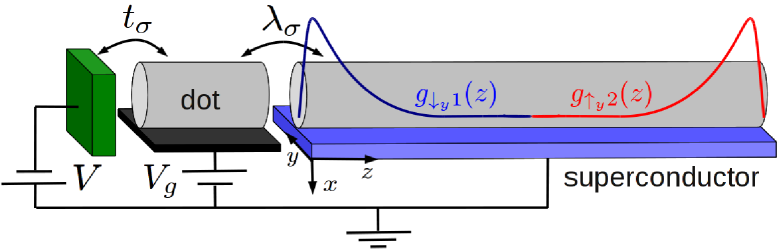
Figure 1: (Color online) Sketch of the proposed setup. An $s$-wave superconductor induces superconductivity in a semiconducting wire with strong spin-orbit coupling. A magnetic field can then induce a topological phase where MBS are formed at the ends of the wire. A quantum dot is formed e.g., by separating a short segment from the main wire by a tunnel barrier, and it is tunnel coupled to a metallic normal lead.

We focus here on a wire-type topological superconductor, which seems experimentally most attractive, but the main conclusions are independent of such details. Systems of several coupled quantum dots and MBS have been suggested as probes of the non-locality of Majorana Fermions Tewari08 and very recently as an alternative way to perform non-Abelian rotations within the degenerate Majorana groundstate manifold Flensberg10b . However, the non-equilibrium transport properties of a normal metal–quantum dot–MBS junction have to our knowledge not been investigated previously and therefore the possibility to probe the parity lifetime in such a setup has also not been discovered. As we will show, even a small coupling between the two MBS strongly suppresses the current. A finite parity relaxation rate partially restores the current but qualitatively changes the transport spectrum, allowing a finite lifetime to be detected, and in addition its precise value can be measured if the MBS coupling or tunnel rates can be controlled.

We solve exactly the problem of a strongly interacting quantum dot coupled to a MBS and treat the coupling to the normal metal perturbatively, yielding a set of master equations for the state of the combined dot–MBS system. From these equations we calculate the non-linear current as a function of the bias voltage applied to the normal lead and of the gate voltage which controls the quantum dot energy. In addition, in the supporting information we provide an exact solution of the transport problem for the case of a non-interacting quantum dot EPAPS .

The basic properties of MBS in semiconducting systems with induced superconductivity have been described in e.g., Refs. Oreg10 ; Alicea10 ; Lutchyn10 ; Sau10 . For suitable parameters, MBS are formed at the ends of the wire, see Fig. 1. These are zero-energy solutions to the Boguliubov de Genne equations and are described by the operators

$$\gamma_{m} = \int dz\sum_{\sigma}\left(g_{\sigma m}(z)\Psi_{\sigma}(z)+g_{\sigma m}^{*}(z)\Psi_{\sigma}^{\dagger}(z)\right),$$ (1)

where $\Psi_{\sigma}^{\dagger}(z)$ creates an electron with spin projection $\sigma=\uparrow,\downarrow$ at position $z$ in the wire. The exact form of the envelope functions $g_{\sigma m}(z)$, describing the spatial form of the MBS, depends on the details of the wire, but $g_{\sigma 1}$ and $g_{\sigma 2}$ have their main weight close to opposite ends and decay exponentially inside the wire. Clearly, the MBS operators satisfy $\gamma_{m}=\gamma_{m}^{\dagger}$ and we assume them to be normalized, such that $\gamma_{1}\gamma_{2}=-\gamma_{2}\gamma_{1}$, $\gamma_{m}^{2}=1$. One end of the wire is tunnel coupled to a quantum dot. The coupled dot–MBS system is described by

$$H_{0} = H_{D}+\frac{i}{2}\xi\gamma_{1}\gamma_{2}+\sum_{\sigma}\left(\lambda_{\sigma}d_{\sigma}-\lambda_{\sigma}^{*}d_{\sigma}^{\dagger}\right)\gamma_{1},$$ (2)

where $H_{D}=\sum_{\sigma}\epsilon_{\sigma}n_{\sigma}+Un_{\uparrow}n_{\downarrow}$ describes the dot, $n_{\sigma}=d_{\sigma}^{\dagger}d_{\sigma}$ is the number operator, and $U$ is the Coulomb charging energy for electrons on the dot. The low-energy Hamiltonian describing the two MBS was discussed in Ref. Kitaev01 and has been used in a transport setup in e.g., Refs. Tewari08 ; Lutchyn10 ; Bolech07 ; Flensberg10 ; Law09 ; the coupling of the two MBS is given by $\xi$, and $\lambda_{\sigma}$ is the coupling between electrons on the dot and the MBS at the corresponding end of the wire. To be specific, we assume the wire to have a Rashba-type spin-orbit coupling along the $x$-direction, and apply a magnetic field $B$ along $z$, leading to a Zeeman splitting on the dot, $\Delta_{B}=\epsilon_{\uparrow}-\epsilon_{\downarrow}$. For definiteness, we take the MBS wave function at the dot side of the wire to be $\propto\Psi_{\downarrow_{y}}^{\dagger}(z)+\Psi_{\downarrow_{y}}(z)$ (see e.g., Oreg10 ), where $\downarrow_{y}$ means spin along the negative $y$-axis, and therefore couples only to the $y$-component of the dot spin, equal in amplitude but different in phase for the two dot spin directions, $\lambda_{\uparrow}=\lambda$, $\lambda_{\downarrow}=-i\lambda$. The metallic normal lead is described by $H_{N}=\sum_{k\sigma}\epsilon_{k}c_{k\sigma}^{\dagger}c_{k\sigma}$ and it couples to the dot via $H_{T}=\sum_{k\sigma}t_{k}d_{\sigma}c_{k\sigma}^{\dagger}+h.c.$, where $c_{k\sigma}^{\dagger}$ creates an electron in the normal lead with energy $\epsilon_{k}$, and where $t_{k}$ is the amplitude for dot$\leftrightarrow$normal lead tunneling.

It is useful to switch to a representation where the two Majorana Fermions are combined to form one ordinary Fermion: $\gamma_{1}=f+f^{\dagger}$, $\gamma_{2}=i(f^{\dagger}-f)$, where $f^{\dagger}$ creates a Fermion and $f^{\dagger}f=0,1$ counts the occupation of the corresponding state. The Hamiltonian (2) now becomes

$$H_{0} = H_{D}+\xi\left(f^{\dagger}f-\frac{1}{2}\right)$$ (3)

$$+ \sum_{\sigma}\left(\lambda_{\sigma}d_{\sigma}f^{\dagger}+\lambda_{\sigma}d_{\sigma}f+h.c.\right),$$

When $\lambda=0$, the eigenstates of (3) are given by $|n_{d}n_{f}\rangle$, where $n_{d}=0,\uparrow,\downarrow,2$ and $n_{f}=0,1$ describe the states of the dot and the MBS system, respectively. Also when $\lambda\neq 0$, the Hamiltonian (3) is block-diagonal in this basis, with an even block $H_{0}^{(e)}$, acting on $|00\rangle,|\sigma 1\rangle,|20\rangle$, and an odd block $H_{0}^{(o)}$, acting on $|\sigma 0\rangle,|01\rangle,|21\rangle$. Fermion number is not conserved by (3), but, because of the block-structure, the parity of the total Fermion number of the dot–MBS system is conserved. When $\xi=0$, $H_{0}^{(e)}$ and $H_{0}^{(o)}$ are identical, $\xi\neq 0$ breaks this parity symmetry.

Diagonalizing (3) yields odd/even parity eigenstates $|o_{i}/e_{i}\rangle=\sum_{n_{d}n_{f}\in o/e}\alpha^{o_{i}/e_{i}}_{n_{d}n_{f}}|n_{d}n_{f}\rangle$. The tunnel Hamiltonian, $H_{T}$, changes the dot electron number by $\pm 1$ and thus connects the even and odd parity sections: $\langle e_{i}|H_{T}|o_{j}\rangle=\sum_{k\sigma}K_{k\sigma}^{e_{i}o_{j}}c_{k\sigma}^{\dagger}+h.c.$, where the many-body tunnel matrix elements are given by

$$K_{k\sigma}^{e_{i}o_{j}} = t_{k}\sum_{\begin{subarray}{c}n_{d}n_{f}\in e\\ n_{d}^{\prime}n_{f}^{\prime}\in o\end{subarray}}\alpha^{e_{i}*}_{n_{d}n_{f}}\alpha^{o_{j}}_{n_{d}^{\prime}n_{f}^{\prime}}\langle n_{d}n_{f}|d_{\sigma}|n_{d}^{\prime}n_{f}^{\prime}\rangle.$$ (4)

In the presence of strong electron–electron interactions, the tunneling between the normal lead and the dot–MBS system cannot be solved exactly (in the limit $U=0$ we provide an exact solution in the supporting information EPAPS ). To leading order in $H_{T}$, the problem can be formulated in terms of master equations Bruus04book , which we modify to account for the lack of particle conservation. The occupations $P_{a}$ of the dot–MBS eigenstates $|a\rangle=|e_{i}\rangle,|o_{i}\rangle$ are calculated from

$$0 = \sum_{a^{\prime}}\left(W_{aa^{\prime}}P_{a^{\prime}}-W_{a^{\prime}a}P_{a}\right),\;\;\sum_{a}P_{a}=1,$$ (5)

$$W_{aa^{\prime}} = \sum_{\sigma}\left\{\Gamma_{\sigma}^{aa^{\prime}}F\left(E_{aa^{\prime}}\right)+\Gamma_{\sigma}^{a^{\prime}a}\left[1-F\left(E_{a^{\prime}a}\right)\right]\right\},$$ (6)

where $E_{aa^{\prime}}=E_{a}-E_{a^{\prime}}$, with $E_{a}$ the energy of eigenstate $|a\rangle$, and $F(E)=1/(e^{(E-\mu_{N})/T}+1)$ is the Fermi function of the normal lead with electron temperature $T$ and chemical potential $\mu_{N}=V$. (We set $k_{B}=e=\hbar=1$.) The tunnel couplings are $\Gamma_{\sigma}^{aa^{\prime}}=2\pi\rho_{N}|K_{\sigma}^{aa^{\prime}}|^{2}$, with $\rho_{N}$ being the density of states in the normal lead. Note that due to the lack of particle conservation, any pair of states $a,a^{\prime}$ are connected both by processes removing and adding an electron to the normal lead, described by the first and second term in Eq. (6) respectively. We here assumed energy independent density of states and tunnel amplitude, but the eigenstates $a,a^{\prime}$ depend on the dot level position and the effective tunnel couplings $\Gamma_{\sigma}^{aa^{\prime}}$ vary between $0$ and $2\pi\rho_{N}|t|^{2}=\Gamma$. The physics described by Eq. (5) is easily understood. The occupation probability of state $a$ is given by the sum of all tunnel processes starting from any state $a^{\prime}$ and ending with occupation of state $a$ (first term), minus all processes depopulating state $a$ (second term). The occupations are normalized to one. Note that the rates in Eq. (6) describe electron tunneling only, rates related to parity relaxation can be added to $W_{aa^{\prime}}$ as described below. The particle current flowing into the dot from the normal lead is given by $I=\sum_{aa^{\prime}}W_{aa^{\prime}}^{I}P_{a^{\prime}}$, where the current rate matrix $W_{aa^{\prime}}^{I}$ is similar to (6), but with a minus sign on the second term, corresponding to electrons tunneling into the normal lead.

The restriction to lowest order perturbation theory is valid when $T\gg\Gamma$. In addition, we neglected off-diagonal elements of the density matrix, valid when all eigenstates are well separated on a scale set by the tunnel broadening, satisfied when $\lambda\gg\Gamma$. Neglecting all states in the superconductor except the MBS is valid when the induced superconducting gap $\Delta$ is larger than the other energy scales. Moreover, $U$ can be several meV in small quantum dots formed in semiconducting wires Jespersen06 ; Nilsson09 , which is likely $\gtrsim\Delta$, and the same holds for the level-spacing, motivating the single-orbital model used here.

Next, we present solutions of the master equations for specific choices of parameters, and with the above energy scales and limitations in mind, we take $U=\infty$ and $T=\lambda=10\Gamma=\Delta_{B}/100$, with $T\lesssim 100$ mK. The voltage-dependence of the energy cost for adding an electron to the dot can be included in the orbital energies, $(\epsilon_{\downarrow}+\epsilon_{\uparrow})/2=\epsilon_{0}-\alpha V_{g}+\beta V$, where $\alpha$ (gate coupling) and $\beta$ depend on the capacitances associated with the dot–superconductor and dot–normal metal tunnel junctions. We take $\beta=1/2$ and $\epsilon_{0}=0$ (other choices affect only the slope and absolute position of resonances, respectively). The differential conductance, $dI/dV$, plotted on color scale as function of $V$ and $V_{g}$ (”stability diagram”), is shown in Fig. 2 for different values of $\lambda$ and $\xi$.

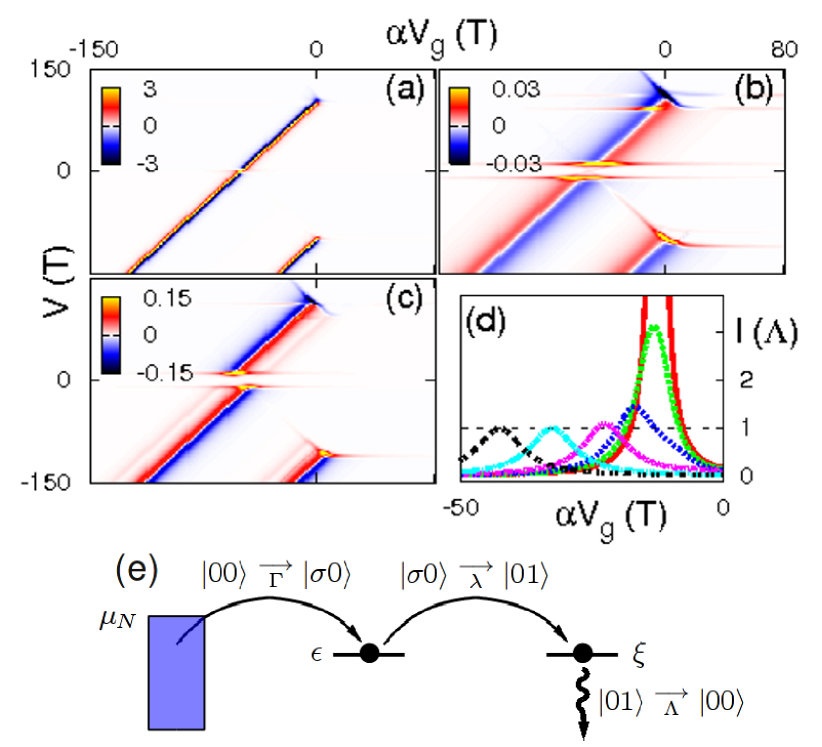
Figure 2: (Color online) Stability diagrams: $dI/dV$ normalized by $0.02e^{2}/h$, plotted on color scale as function of $V$ and $V_{g}$, with (a): $\xi=0$, (b): $\xi=10T$, (c): $\xi=10T$ and finite parity relaxation, $\Lambda=0.04\Gamma$. Note the different scales in (b) and (c) showing the dramatic effect of the finite parity lifetime and the characteristic shift in gate voltage position between the positive and negative bias peaks in (c). (d): $I(V_{g})$ at $V=75T$ with parameters as in (c), but increasing $\xi/\lambda=0,2.5,5,10,20,30$ (increasing as indicated by the arrow). For $\Lambda\gg\Gamma\lambda^{2}/\xi^{2}$, $\Lambda$ can be read off directly from the height of the shifted current peaks. (e): Sketch of resonant transport processes for $\epsilon=\xi$ when $V>0$ in (c). Similar resonant processes exist for $\epsilon=-\xi$ when $V<0$.

To develop an understanding of the physics underlaying the stability diagrams, we consider first the case without parity relaxation, described by Eqs. (5) and (6). We start with the simplest case of $\xi=0$, see Fig. 2(a). A significant current can only flow when one of the dot spin states is energetically aligned with the MBS, allowing electrons to tunnel resonantly between the dot and superconductor, resulting in a current peak of width $\sim\lambda$ and height $I_{\text{max}}=\Gamma/2$ and therefore in narrowly spaced positive and negative conductance lines. Thus, the sharp nature of the MBS gives rise to negative differential resistance in transport through the dot. The peak associated with $\sigma=\uparrow$ terminates at large positive $V$, when an electron can tunnel from the normal lead into the $\sigma=\downarrow$ state, blocking transport through the $\sigma=\uparrow$ channel (via the Coulomb charging energy) since it cannot tunnel out again into the normal lead (due to energy conservation) or into the MBS (due to the energy mis-match). Similarly, the $\sigma=\downarrow$ peak vanishes above a negative threshold $V$, when $\sigma=\uparrow$ falls below $\mu_{N}$. Thus, properly accounting for Coulomb blockade is essential to understand the qualitative conductance features. In Fig. 2(b), a finite $\xi$ introduces an energy splitting between the even and odd parity sectors, suppressing the current for $|V|<\xi$. Even for $|V|>\xi$ the conductance is significantly lower compared to $\xi=0$ [note the different scales in Figs. 2(a) and (b)]. To understand why, consider e.g., electrons being transported from the normal lead to the superconductor ($V>0$) by sequential tunneling through the dot, which in the basis of the unperturbed number states $|n_{d}n_{f}\rangle$ involves the processes: $|00\rangle\;\begin{subarray}{c}\longrightarrow\\ \Gamma\end{subarray}\;|\sigma 0\rangle\;\begin{subarray}{c}\longrightarrow\\ \lambda\end{subarray}\;|01\rangle\;\begin{subarray}{c}\longrightarrow\\ \Gamma\end{subarray}\;|\sigma 1\rangle\;\begin{subarray}{c}\longrightarrow\\ \lambda\end{subarray}\;|00\rangle$. Because we consider here the case without parity relaxation in the superconductor, any process changing the parity of the dot–MBS system must involve tunneling to/from the normal lead, and therefore two electrons are transferred before the system returns to its initial state. When the even–odd degeneracy is split by $\xi\neq 0$, both dot–MBS tunnel processes cannot be resonant at the same voltage, suppressing the conductance by a factor $\propto\lambda^{2}/\xi^{2}$. Instead, horizontal conductance lines appear, corresponding to inelastic cotunneling DeFranceschi01 through the dot, exciting the parity degree of freedom, i.e., a direct processes $|00\rangle\;\begin{subarray}{c}\longrightarrow\\ \Gamma\lambda\end{subarray}\;|01\rangle$, energetically allowed for $|V|>\xi$ and involving only virtual occupation of the intermediate state $|\sigma 0\rangle$. Note that all tunnel process $\propto\Gamma\lambda^{n}$ are included in our master equations, since the dot–MBS coupling is treated exactly. Interestingly, due to the sharp MBS, inelastic cotunneling gives rise to conductance peaks, rather than steps. Similarly, horizontal lines at $V=\pm\Delta_{B}$ correspond to inelastic cotunneling exciting the dot, e.g., $|\uparrow 0\rangle\;\begin{subarray}{c}\longrightarrow\\ \lambda\Gamma\end{subarray}\;|\downarrow 0\rangle$.

Next, we introduce a finite relaxation of the Fermion parity in the superconductor, caused by quasiparticle poisoning Mannik04 ; Aumentado04 , and show that this has a striking effect on the stability diagrams. Rather than starting from a microscopic model of the quasiparticle generation, we focus on the generic effects and assume that transitions between dot–MBS eigenstates $|a^{\prime}\rangle\rightarrow|a\rangle$ are induced with rate $\Lambda_{aa^{\prime}}$ if $E_{a^{\prime}}>E_{a}$ and rate $\Lambda_{aa^{\prime}}\text{exp}[(E_{a^{\prime}}-E_{a})/T]$ otherwise, where $\Lambda_{aa^{\prime}}$ is obtained by assuming a rate $\Lambda$ for transitions $|n_{d}n_{f}\rangle\rightarrow|n_{d}\bar{n}_{f}\rangle$ ($\bar{1}=0,\bar{0}=1$), and then transforming to the dot–MBS eigenbasis, cf., Eq. (4). These rates are then added to the rate matrix in Eq. (6). As is seen by comparing Fig. 2(c) and (b), which differ only by a small such relaxation rate, this has a dramatic effect on the conductance (note the different scales). To understand the increased conductance, consider transport at $V>0$, which for $\Lambda\neq 0$ is dominated by the processes: $|00\rangle\;\begin{subarray}{c}\longrightarrow\\ \Gamma\end{subarray}\;|\sigma 0\rangle\;\begin{subarray}{c}\longrightarrow\\ \lambda\end{subarray}\;|01\rangle\;\begin{subarray}{c}\longrightarrow\\ \Lambda\end{subarray}\;|00\rangle$, see sketch in Fig. 2(e). Hence, parity relaxation allows the total dot–MBS system to return to its initial state after transferring only a single electron, and this electron tunnels through the system fully resonantly when $\epsilon_{\sigma}=\xi$. Similarly, at $V<0$ transport is dominated by: $|00\rangle\;\begin{subarray}{c}\longrightarrow\\ \lambda\end{subarray}\;|\sigma 1\rangle\;\begin{subarray}{c}\longrightarrow\\ \Lambda\end{subarray}\;|\sigma 0\rangle\;\begin{subarray}{c}\longrightarrow\\ \Gamma\end{subarray}\;|00\rangle$, which is fully resonant at $\epsilon_{\sigma}=-\xi$. Thus, parity relaxation leads to resonant transport even for finite $\xi$, but the resonance condition is different for positive and negative bias and therefore the peaks are shifted by $2\xi$.

The shifted peak behavior is observed when the parity relaxation rate exceeds the suppressed transport rates discussed in connection with Fig. 2(b), i.e., when $\Lambda\gtrsim\Gamma\lambda^{2}/\xi^{2}$. If, in addition, $\Gamma\gg\Lambda$, parity relaxation is the slowest process in Fig. 2(e) and the peak current is equal to $\Lambda$ maxcurrent . Experimentally, $\xi$ could be changed by moving the MBS corresponding to $\gamma_{2}$ with ”keyboard” gates as suggested in Ref. Alicea10b . $I(V_{g})$ curves for increasing $\xi$ are shown in Fig. 2(d), allowing the parity relaxation to be directly read off from the height of the current peaks at large $\xi$. Alternatively, one could change instead $\Gamma$ and/or $\lambda$ via additional gates. Note that $\Lambda$ can be directly measured without knowing the precise values of e.g., $\Gamma$ and $\lambda$. We emphasize that even at finite $\xi$, the two-Majorana state described by $\gamma_{1,2}$ or $f^{\dagger},f$ can only relax by also changing the parity of the superconductor. Therefore, even though our proposed measurement has to be done at finite $\xi$, the relaxation rate measured is the parity relaxation rate, which is arguably independent of $\xi$.

In conclusion, we have suggested a relatively simple setup in which to measure the lifetime of the parity of a Majorana system, being of crucial importance in topological quantum computing schemes Nayak08rev . Our suggestion does not involve (experimentally problematic) interferometry or braiding operations. Thus, one can test different realizations of topological superconductors and different material choices, selecting the most suitable ones, before going through the difficult process of actually constructing a topological quantum computer. The setup we propose is a normal metal–quantum dot–topological superconductor junction. We have calculated the non-linear conductance of this system as a function of the applied gate and bias voltages within a master equation approach and shown that the lifetime of the parity of the Majorana system can be directly read off from the height of the current peaks at finite Majorana coupling.

We thank Harvard University, where part of this work was done, for hospitality. This work was funded in part by The Danish Council for Independent Research $|$ Natural Sciences and by Microsoft Corporation Project Q.

Supplementary information

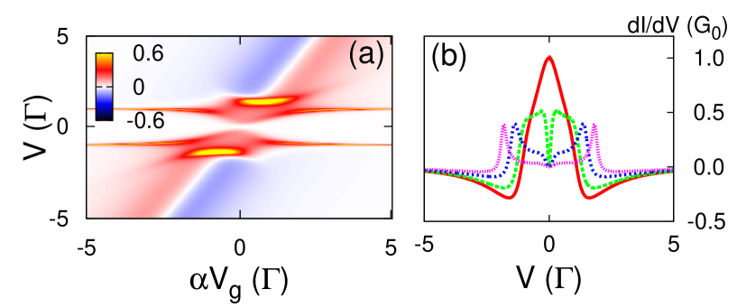
Figure 3: (Color online) (a) $dI/dV$ normalized by $2e^{2}/h$, plotted on color scale as function of $V$ and $V_{g}$, with $\xi=\Gamma=2\lambda$, $T=0$. We take the voltage coupling $\beta=1/2$ as in Fig. 2 in the main paper, but choose the gate voltage scale such that $\epsilon_{\uparrow}=0$ when $V_{g}=V=0$. (b) $dI/dV$ as function of $V$ at $V_{g}=0$. The parameters are the same as in (a), except for $\xi$ which is varied: $\xi=0$ (red solid line), $\xi=\Gamma/2$ (green dashed line), $\xi=\Gamma$ (blue dotted line), $\xi=3\Gamma/2$ (purple fine dotted line).

We here consider the Zeeman splitting to be the largest energy scale, $\Delta_{B}\gg|V|,T,\Gamma,\lambda$, in which case transport through the ground state of the dot can be described by a non-interacting model and solved exactly using a Green’s function approach. The current can be written as

$$I = -\Gamma\int\frac{d\omega}{2\pi}\;\left[2\text{Im}G^{R}_{dd}+\Gamma\left(|G^{R}_{dd}|^{2}-|F^{R}_{dd}|^{2}\right)\right]$$ (7)

$$\times \left[F(\omega)-F_{0}(\omega)\right],$$

where $F_{0}(\omega)$ is the Fermi function at $V=0$, $G^{R}_{dd}$ is the Fourier transform of the retarded dot Green’s function for $\sigma=\uparrow$ electrons, and $F^{R}_{dd}(t-t^{\prime})=-i\theta(t-t^{\prime})\langle\{d_{\uparrow}(t),d_{\uparrow}(t^{\prime})\}\rangle$ is the corresponding anomalous Green’s function. (We here only consider $\Lambda=0$.) Next, we take the time derivative of $G^{R}_{dd}(t-t^{\prime})$ [and of all Green’s functions appearing when doing so, including $F^{R}_{dd}(t-t^{\prime})$], Fourier transform, and solve the resulting equations of motion, which gives

$$G^{R}_{dd}=\frac{1}{\omega-\epsilon_{\uparrow}+\frac{i}{2}\Gamma-2|\lambda|^{2}M(\omega)\left[1+2|\lambda|^{2}\tilde{M}(\omega)\right]},$$ (8)

$$F^{R}_{dd}=\\ \frac{-2(\lambda^{*})^{2}M(\omega)}{\left(\omega+\epsilon_{\uparrow}+\frac{i}{2}\Gamma\right)\left(\omega-\epsilon_{\uparrow}+\frac{i}{2}\Gamma\right)-4|\lambda|^{2}\left(\omega+\frac{i}{2}\Gamma\right)M(\omega)},$$ (9)

where $M(\omega)=1/(\omega-\xi^{2}/\omega)$, and $\tilde{M}(\omega)=M(\omega)/[\omega+\epsilon_{\uparrow}+\frac{i}{2}\Gamma-2|\lambda|^{2}M(\omega)]$.

When $\lambda,T\gg\Gamma$, the results agree fully with the master equation results for $B=\infty$ and we now focus instead on the limit $T=0,\lambda\lesssim\Gamma$. Figure 3(a) shows a stability diagram similar to those in Fig. 2 in the main paper, but for a smaller voltage window close to the $\epsilon_{\uparrow}=0$ crossing.

Figure 3(b) shows $dI/dV$ as function of $V$ at $V_{g}=0$, for varying values of $\xi$. The zero-bias conductance, $G(0)$, can be found analytically from (7). When $\xi=0$, we always have $G(0)=2e^{2}/h$, independent of $V_{g}$, although the width of the peak decreases when the dot level is brought out of resonance. Conversely, for any $\xi\neq 0$, we find $G(0)=0$, independent of $V_{g}$. This is similar to the linear conductance of a normal metal–MBS tunnel junction, see Ref. [16] of the main paper. At finite $\xi$, peaks instead appear at finite voltage $V\approx\pm\xi$, as discussed in connection with the master equation results in the main paper, and close to $V_{g}=0$ an interesting double peak structure is found.

References

- (1) A. Stern, Nature 464, 187 (2010)
- (2) C. Nayak, S. H. Simon, A. Stern, M. Freedman, and S. Das Sarma, Rev. Mod. Phys. 80, 1083 (2008)
- (3) G. Moore and N. Read, Nucl. Phys. B 360, 362 (1991)
- (4) Y. E. Kraus, A. Auerbach, H. A. Fertig, and S. H. Simon, Phys. Rev. B 79, 134515 (2009)
- (5) L. Fu and C. L. Kane, Phys. Rev. Lett. 100, 096407 (2008)
- (6) J. D. Sau, R. M. Lutchyn, S. Tewari, and S. Das Sarma, Phys. Rev. Lett. 104, 040502 (2010)
- (7) J. Alicea, Phys. Rev. B 81, 125318 (2010)
- (8) A. R. Akhmerov, J. P. Dahlhaus, F. Hassler, M. Wimmer, and C. W. J. Beenakker, Phys. Rev. Lett. 106, 057001 (2011)
- (9) Y. Oreg, G. Refael, and F. von Oppen, Phys. Rev. Lett. 105, 177002 (2010)
- (10) R. M. Lutchyn, J. D. Sau, and S. Das Sarma, Phys. Rev. Lett. 105, 077001 (2010)
- (11) A. Y. Kitaev, Physics-Uspekhi 44, 131 (2001)
- (12) J. D. Sau, S. Tewari, and S. Das Sarma, Phys. Rev. A 82, 052322 (2010)
- (13) J. Alicea, Y. Oreg, G. Refael, F. von Oppen, and M. P. A. Fisher, Nature Physics 7, 412 (2011)
- (14) C. J. Bolech and E. Demler, Phys. Rev. Lett. 98, 237002 (2007)
- (15) K. T. Law, P. A. Lee, and T. K. Ng, Phys. Rev. Lett. 103, 237001 (2009)
- (16) K. Flensberg, Phys. Rev. B 82, 180516(R) (2010)
- (17) J. Männik and J. E. Lukens, Phys. Rev. Lett. 92, 057004 (2004)
- (18) J. Aumentado, M. W. Keller, J. M. Martinis, and M. H. Devoret, Phys. Rev. Lett. 92, 066802 (2004)
- (19) S. Tewari, C. Zhang, S. Das Sarma, C. Nayak, and D.-H. Lee, Phys. Rev. Lett. 100, 027001 (2008)
- (20) K. Flensberg, Phys. Rev. Lett. 106, 090503 (2011)
- (21) See supplementary information for an exact Green’s function solution of the transport problem in the limit of a non-interacting quantum dot.
- (22) H. Bruus and K. Flensberg, Many-Body Quantum Theory in Condensed Matter Physics (Oxford University Press, 2004)
- (23) T. S. Jespersen, M. Aagesen, C. Sørensen, P. E. Lindelof, and J. Nygård, Phys. Rev. B 74, 233304 (2006)
- (24) H. A. Nilsson, P. Caroff, C. Thelander, M. Larsson, J. B. Wagner, L.-E. Wernersson, L. Samuelson, and H. Q. Xu, Nano Lett. 9, 3151 (2009)
- (25) S. DeFranceschi, S. Sasaki, J. M. Elzerman, W. G. van der Wiel, S. Tarucha, and L. P. Kouwenhoven, Phys. Rev. Lett. 86, 878 (2001)
- (26) For , the peak current expanded in and is