Skewed superstatistical distributions from a Langevin and Fokker-Planck approach

Abstract

The superstatistics concept is a useful statistical method to describe inhomogeneous complex systems for which a system parameter $\beta$ fluctuates on a large spatio-temporal scale. In this paper we analyze a measured time series of wind speed fluctuations and extract the superstatistical distribution function $f(\beta)$ directly from the data. We construct suitable Langevin and Fokker-Planck models with a position dependent $\beta$-field and show that they reduce to standard type of superstatistics in the overdamped limit.

I Introduction

The superstatistics concept introduced in 2003 beck-cohen provides a useful tool to describe a large variety of complex systems (unicla, ; touchette, ; supergen, ; souza, ; chavanis, ; vignat, ; Plastino-x, ; jizba, ; prl01, ; frank, ; hase, ; celia, ; abul-again, ; straeten-recent, ). The basic idea is to characterize the complex system under consideration by a superposition of two statistics, one corresponding to ordinary statistical mechanics (on a mesoscopic level modeled e.g. by a Langevin equation) and the other one corresponding to a slowly varying parameter $\beta(\vec{x},t)$ of the system which can be, but need not to be, an inverse temperature. There are many interesting applications of superstatistical techniques. Recent work in this direction includes train delay statistics briggs , the distribution of accelerations of test particles in turbulent flows prl and cancer survival statistics chen . Further applications are described in (daniels, ; maya, ; reynolds, ; RMT, ; abul-magd3, ; porpo, ; rapisarda, ; kantz, ; cosmic, ; eco, ; vdsbeck1, ; superscatter, ; ausloos, ; kings, ; laub, ; abe-thurner, ; queiros, ; abul-magd2, ; abc, ; crooks, ; naudts, ; straeten, ; hau, ).

In this paper, as a working example, we study measured statistics of wind speed fluctuations. For previous work in this direction, see rapisarda ; kantz . We will extract the superstatistical distribution function $f(\beta)$ out of our data set and show that in good approximation it is an inverse gamma distribution. As a theoretical model for these and other data sets, we will study Langevin and Fokker-Planck equations with a varying, position-dependent $\beta$. We will show that in the overdamped limit these models reduce to standard type of superstatistics. Skewed stationary distributions arise naturally in these types of models if the overdamped limit is not completely performed.

This paper is organized as follows. In section II we recall the basic concepts of superstatistics, illustrated with the example of a linear Langevin equation. In section III we apply our methods to measured wind speed data, extracting various relevant distributions and parameters out of the data set. In section IV we extend our theoretical approach by studying a Kramers-like equation with spatially varying $\beta$. We show that this model reduces to standard type of superstatistics in the overdamped limit. An example is studied in section V. Then, in section VI we comment on the skewness of the generated distributions. The last section gives a short discussion of the results of this paper.

II Linear Langevin equation with time-dependent $\beta$

Let us study as a simple example the following Langevin equation

$$\frac{d}{dt}v(t) = -\gamma v(t)+\sqrt{\frac{2\gamma}{m}\frac{1}{\beta(t)}}g(t),$$ (1)

where $\gamma$ and $m$ are constants and $g(t)$ corresponds to Gaussian white noise with unit variance. $v(t)$ is a stochastic process that can be associated with the velocity of a Brownian particle. If $\beta(t)=\beta$ is a constant, then one ends up with the standard Langevin equation which describes the dynamical process of a Brownian particle with mass $m$ in an environment with constant temperature $1/\beta$. It is well known that the stationary velocity distribution of a Brownian particle is a Gaussian distribution with zero mean and variance $1/\beta$. The relaxation time is $\tau=1/\gamma$. In superstatistics, one considers a Brownian particle moving through an environment with a slowly fluctuating temperature field whose changes take place on a typical time scale $T$ such that $\tau<<T$. When this inequality holds, the local velocity distribution of the system can relax to a Gaussian distribution before the next change of $\beta(t)$ takes place. As such, after a long time, the stationary velocity distribution $P(v)$ of the particle is just a superposition of Gaussian distributions weighted with a function $f(\beta)$

$$P(v) \approx \int_{\beta_{\textrm{min}}}^{\beta_{\textrm{max}}}d\beta f(\beta)\sqrt{\frac{m\beta}{2\pi}}\exp\left(-\frac{1}{2}m\beta v^{2}\right).$$ (2)

This $f(\beta)$ is the probability density to observe some value of $\beta$. Depending on the properties of $f(\beta)$, different results for the stationary velocity distribution $P(v)$ will occur touchette , e.g., power-laws or stretched exponentials. In unicla ; vdsbeck1 a method was introduced to determine $f(\beta)$, given an experimental time series. The method extracts the main superstatistical parameters out of a given data set and examines the validity of the superstatistical model assumptions. Depending on the system under study, one can obtain different results for $f(\beta)$. We will first briefly outline this method to extract $f(\beta)$ from the data.

The starting point is a discrete time series $v$ containing $n$ data points. Using the definitions proposed in unicla ; vdsbeck1 , one can estimate values for the two different time scales $\tau$ and $T$. In case that the inequality $\tau/T<<1$ holds, one proceeds by dividing the time series $v$ in $N$ different time slices of length $t$ with $N=\lfloor n/t\rfloor$, where $\lfloor x\rfloor$ means rounding the value of $x$ to the nearest lower integer. Then, one calculates the variance of $v$ in each of these sub-intervals. The inverse of the variance is an estimator for the value of $\beta$. As such, one obtains a new series containing $N$ points which are denoted as $\beta_{i}$ with $i=1,2,\ldots N$. Within this assumption, the distribution $P(v)$ is approximated by

$$P(v)\approx\frac{1}{N}\sum_{i=1}^{N}\sqrt{\frac{\beta_{i}}{2\pi}}e^{-\frac{1}{2}\beta_{i}v^{2}}.$$ (3)

When $N$ is large enough, one can replace expression (3) by (2) with $f(\beta)$ being the probability density that the value of the inverse variance in a randomly chosen time slice of length $T$ equals $\beta$. Notice that the superstatistical approach includes two approximations. In the first step, one assumes the existence of two time scales $\tau$ and $T$ such that in every time slice ’local’ equilibrium is reached. Then, $P(v)$ can be approximated by (3). In the second step one assumes the existence of a distribution $f(\beta)$ replacing the summation in expression (3) by an integral. Then, $P(v)$ can be approximated by (2).

III Application to wind speed fluctuations

In the following, as a working example, we apply our method to an experimentally measured time series of the horizontal component $v(t)$ of wind speeds recorded af the Lammefjord site at a height of 10m (cup 1) during the year 1987 wind-data . The incremental distribution of $u_{\delta}(t):=v(t+\delta)-v(t)$ exhibits non-Gaussian behavior that can be modelled using superstatistics laub . As an illustration, we calculated the superstatistical approximation of the incremental distribution ($\delta=8$) of the windspeeds at day $191$. The measuring frequency is $8$Hz. This means that the number of data points is $n=24\times 3600\times 8\approx 7\times 10^{5}$. The two different time scales extracted from the data are $\tau\approx 4.1$ and $T\approx 112$, obtained by using similar techniques as in unicla ; vdsbeck1 . This illustrates that the data set shows clear time scale separation, in agreement with the results of kantz . Knowing the value of $T$, one can construct the distribution $f(\beta)$ and try to approximate this histogram with some well-known distributions such as the gamma distribution, the lognormal distribution or the inverse gamma distribution. The latter one is given by

$$f(\beta) = \frac{\theta^{\alpha}}{\Gamma(\alpha)}\beta^{-\alpha-1}e^{-\theta/\beta}.$$ (4)

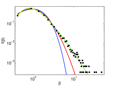
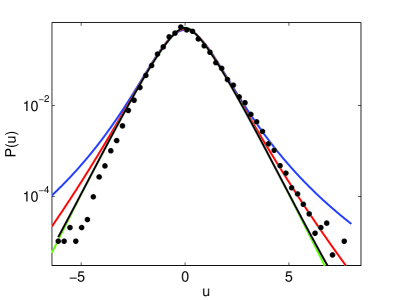
Here $\alpha$ and $\theta$ are parameters. The relevance of the above three distributions was motivated in unicla . The results of our calculations are shown in figure 1. There is an excellent agreement between the histogram extracted from the data and the inverse gamma distribution. The right part of the figure also shows the empirical distribution $P(u)$ together with the first and second approximation of superstatistics given by eqs. (3) and (2), respectively. The first approximation of superstatistics well models the fat tails of the empirical distribution $P(u)$, see Figure 1. The excellent agreement between $P(u)$ and expression (2), with $f(\beta)$ being the inverse gamma distribution, gives further evidence that this latter distribution is well able to represent the fluctuations of $\beta$. Summarizing, our simple superstatististical model discussed so far is a good first-order approximation of the process of windspeeds increments.

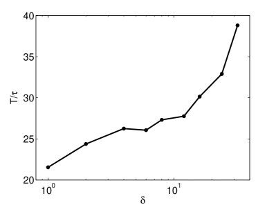
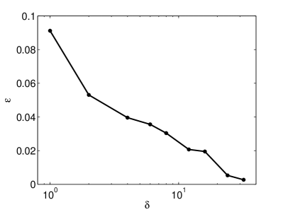
Figure 2 shows the extracted time scale ratio $T/\tau$ as a function of $\delta$. Apparently, for small $\delta$ the time scale separation between $T$ and $\tau$ is less pronounced. The right part of the figure also shows a parameter $\epsilon$ as a function of $\delta$. This $\epsilon$ was defined in vdsbeck1 as a measure of quality of the superstatistical approximation. The smaller $\epsilon$, the better the superstatistical model assumptions are satisfied for the given time series.

Figure 1: (Colour online) LEFT: Plot of the empirical distribution $f(\beta)$ (dots) extracted from the wind data and the best fit to a lognormal distribution (red), gamma distribution (blue) and an inverse gamma distribution (green). RIGHT: Plot of the empirical distribution $P(u)$ together with the first superstatistical approximation (3) (black line). Also the second approximation (2) is shown, where $f(\beta)$ is given by the lognormal distribution (red), the gamma distribution (blue) and the inverse gamma distribution (green).

Figure 2: (Colour online) LEFT: Ratio of the time scales $T$ and $\tau$ as extracted from the data. RIGHT: The parameter $\epsilon$, defined in vdsbeck1 , measures how good a superstatistical model fits a given data set. Ideal superstatistics is corresponding to $\epsilon=0$.

IV Superstatistics and overdamped motion

We will now generalize the Langevin approach to superstatistics. We start from the following set of equations

$$\frac{d}{dt}v(t) = -\gamma v(t)+\frac{1}{m}F(x)+\sqrt{\frac{2\gamma}{m}\frac{1}{\beta(x)}}g(t)$$ (5)

$$\frac{d}{dt}x(t) = v(t),$$ (6)

with $F(x)=-\partial V(x)/\partial x$. Here $V(x)$ is a confining potential like, e.g., a harmonic potential, and $x$ is a position variable. Crucial for our approach is that $\beta$ depends on $x$ but not on the velocity $v$. We are interested in the stationary velocity distribution $P(v)$. It is well known that in case $\beta(x)=\beta$ is a constant, this distribution becomes a Gaussian distribution

$$P(v)=\sqrt{\frac{m\beta}{2\pi}}\exp\left(-\frac{1}{2}m\beta v^{2}\right).$$ (7)

However, we are interested in the general problem where the temperature is position dependent. Then, in order to obtain an exact expression for $P(v)$, one has to solve the corresponding stationary Fokker-Planck equation for the joint distribution $P(v,x)$,

$$0 = \left[\frac{\partial}{\partial v}\left(\gamma v-\frac{1}{m}F(x)\right)-v\frac{\partial}{\partial x}+\frac{\gamma}{m}\frac{1}{\beta(x)}\frac{\partial^{2}}{\partial^{2}v}\right]P(v,x)$$ (8)

and integrate out the dependence of the variable $x$

$$P(v) = \int_{x_{\textrm{min}}}^{x_{\textrm{max}}}dxP(v,x).$$ (9)

The problem with this procedure is that usually it is not possible to obtain an analytical expression for $P(v,x)$. However, in order to make the connection with the superstatistical approach outlined in the previous section, it is not necessary to have the exact form of $P(v,x)$. It is sufficient to study (5) in the high friction limit, i.e., $\gamma\rightarrow\infty$. Taking this overdamped limit of (5) results in a stochastic differential equation in the variable $x(t)$ only:

$$\frac{d}{dt}x(t) = \frac{1}{m\gamma}F(x)+\sqrt{\frac{2}{m\gamma}\frac{1}{\beta(x)}}g(t)$$ (10)

The associated Fokker-Planck equation for the stationary distribution $P_{o}(x)$ becomes

$$0 = -\frac{\partial}{\partial x}F(x)P_{o}(x)+\frac{\partial^{2}}{\partial^{2}x}\frac{1}{\beta(x)}P_{o}(x)$$ (11)

(we used Ito’s interpretation). The lower index $\ {}_{o}$ is used to denote the overdamped limit. Equation (11) can be solved analytically

$$P_{o}(x) = Z^{-1}\beta(x)\exp\left(\int dxF(x)\beta(x)\right),$$ (12)

where $Z$ is a normalization constant. Taking the overdamped limit physically means that the velocity will thermalise very quickly. As a consequence, for large values of $\gamma$, the solution $P(v,x)$ of the complete Fokker-Planck equation (8) is approximated by stolo

$$P(v,x)\approx P_{o}(v,x)=P_{o}(x)P_{o}(v|x).$$ (13)

Here $P_{o}(v|x)$ denotes the conditional distribution of $v$ given the local value of the slow variable $x$. This is just a Gaussian distribution (7) with $\beta$ replaced by $\beta(x)$. As a consequence, one obtains the following approximation for the distribution of interest:

$$P(v)\approx\int_{x_{\textrm{min}}}^{x_{\textrm{max}}}dxP_{0}(v,x)=\int_{x_{\textrm{min}}}^{x_{\textrm{max}}}dxP_{o}(x)\sqrt{\frac{m\beta(x)}{2\pi}}\exp\left(-\frac{1}{2}m\beta(x)v^{2}\right).$$ (14)

After a change of variables, one ends up with (2) in which the superstatistical distribution $f(\beta)$ is associated with

$$\left(\frac{d\beta(x)}{dx}\right)^{-1}P_{o}(\beta(x)).$$ (15)

This shows that the superstatistical approximation is formally equivalent to taking the high friction limit of a stochastic differential equations of type (5). The latter model describes the dynamics of a Brownian particle in an inhomogeneous heat bath in the presence of a confining potential.

V Example

To illustrate the theoretical considerations of the previous section, we study an explicit example here. Assume for simplicity that the temperature is linear in the position $x$. In order to ensure that the temperature remains positive we introduce an arbitrary small positive constant $a$ and define

$$\beta(x)=\frac{1}{|x|+a}, V(x)=\frac{\theta}{2}\left[|x|+a-\frac{\alpha}{\theta}\right]^{2}.$$ (16)

With this choice one obtains for the velocity distribution in the overdamped limit (14)

$$P(v) \approx Z^{-1}\int_{-\infty}^{+\infty}dx\beta(x)\exp\left(-\int dx^{\prime}\frac{\partial V(x^{\prime})}{\partial x^{\prime}}\beta(x^{\prime})\right)\sqrt{\frac{m\beta(x)}{2\pi}}\exp\left(-\frac{1}{2}m\beta(x)v^{2}\right)$$ (17)

$$= Z^{-1}\int_{-\infty}^{+\infty}dx\exp\left((-\alpha+1)\ln\beta(x)-\frac{\theta}{\beta(x)}\right)\sqrt{\frac{m\beta(x)}{2\pi}}\exp\left(-\frac{1}{2}m\beta(x)v^{2}\right)$$ (18)

$$= Z^{-1}\int_{0}^{1/a}d\beta\ \beta^{-\alpha-1}\exp\left(-\frac{\theta}{\beta}\right)\sqrt{\frac{m\beta}{2\pi}}\exp\left(-\frac{1}{2}m\beta v^{2}\right)$$ (19)

where we absorbed constants in the normalization $Z$. In the limit $a\rightarrow 0$, this integral simplifies to

$$P(v) \approx \frac{1}{\Gamma(\alpha)}\sqrt{\frac{2\theta}{\pi}}\left(\sqrt{\frac{\theta}{2}}|v|\right)^{\alpha-1/2}\textrm{K}_{\alpha-1/2}\left(\sqrt{2\theta}|v|\right)$$ (20)

where $\textrm{K}_{\nu}(x)$ is the modified Bessel function of the second kind. Notice that $f(\beta)$ becomes an inverse gamma distribution in this limit. This particular example connects the results of sections III and IV because it shows that the theoretical model of section IV together with the choice (16) for the temperature and the potential reproduces the observed empirical distributions discussed in section III. However, this is only one possibility. In principle, for every choice of $\beta(x)$, a possible candidate for the force that results in an inverse gamma distribution for $f(\beta)$ can be calculated by evaluating the following expression

$$F(x)\beta(x) = -(\alpha+2)\frac{\beta^{\prime}(x)}{\beta(x)}-\theta\frac{\beta^{\prime}(x)}{\beta^{2}(x)}+\frac{\beta^{\prime\prime}(x)}{\beta^{\prime}(x)}.$$ (21)

Where the accent means differentiating with respect to $x$. The reason to chose the particular form of $T(x)$ and $V(x)$ as in (16) is that this is probably the easiest choice that both fulfills equation (21) and is physically meaningful. The latter is also the reason that we introduced the constant $a$ in the expression for the temperature (16). This is to ensure that the particle can pass the origin in the overdamped limit. This problem disappears if one takes finite friction into account. Therefore, it is appropriate to restrict our analysis to the special case $a\rightarrow 0$.

VI Skewness

Figure 3: (Colour online) LEFT: The difference between the empirical distribution $P(u)$ and the second approximation of superstatistics. RIGHT: Kurtosis and skewness of the empirical distribution $P(u)$ as a function of $\delta$.

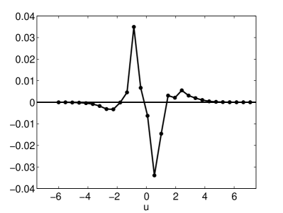
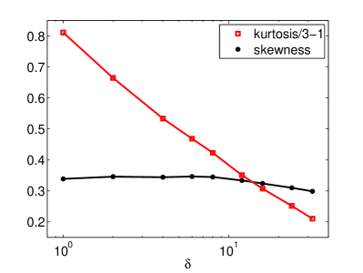
We showed in section III that the superstatistical approach is well suited to describe the fat tails that are exhibited in the wind speed distribution under study. However, it is well known, and clearly visible in figure 1, that the distribution $P(u)$ is slightly skewed (with vanishing first moment). Clearly, the superstatistical distribution (2) is symmetric and can not represent the skewness that occurs in the experimental data. Figure 3 (right part) shows the skewness and kurtosis as a function of $\delta$ for the data set of measured velocity increments $u_{\delta}(t)$. It is possible to model the kurtosis with the superstatistical approach described up till now, however it is impossible to model the skewness.

As mentioned before, the complete Fokker-Planck equation (8) is usually not analytically solvable. However, relations between the moments of the distribution $P(v,x)$ can be obtained, using the Fokker-Planck operator $L$. One has

$$\langle Lv^{i}x^{j}\rangle=0 i,j=0,1,2,\ldots\textrm{with}\,L:=\left(\gamma v-\frac{1}{m}F(x)\right)\frac{\partial}{\partial v}-v\frac{\partial}{\partial x}-\frac{\gamma}{m}\frac{1}{\beta(x)}\frac{\partial^{2}}{\partial^{2}v}.$$ for (22)

Applying this with $i=0,j=1$ results in $\langle v\rangle=0$, while depending on the particular choices of $F(x)$ and $\beta(x)$ one can obtain $\langle v^{3}\rangle\neq 0$. This means that the stationary velocity distribution $P(v)$ can have non-vanishing skewness, while at the same time it has a vanishing first moment. However notice that the overdamped approximation (13) of $P(v,x)$ is symmetric in $v$, regardless of the choice of $\beta(x)$. This means that in order to introduce skewness, one has to go beyond the overdamped limit. Perturbation expansions of $P(v,x)$ around the overdamped limit can be performed stolo . The first order correction is

$$P(v,x) = \sqrt{\frac{m\beta(x)}{2\pi}}\exp\left(-\frac{1}{2}m\beta(x)v^{2}\right)P_{o}(x)\left(1+\frac{1}{6}\frac{1}{\gamma}v\left[m\beta(x)v^{2}-3\right]\frac{1}{\beta(x)}\frac{d\beta(x)}{dx}\right).$$ (23)

Notice that the contribution of the first order correction vanishes for $\langle v^{i}\rangle$ with $i=0,1,2$. The third order moment becomes

$$\langle v^{3}\rangle=\int_{-\infty}^{+\infty}dv\int_{-\infty}^{+\infty}dxv^{3}P(v,x) = \frac{1}{\gamma}\frac{1}{m^{2}}\int_{-\infty}^{+\infty}dxP_{o}(x)\frac{1}{\beta^{3}(x)}\frac{d\beta(x)}{dx}.$$ (24)

This shows that the theoretical model introduced in section IV can be used to systematically describe the experimental data. The superstatistical approximation (the overdamped limit) is used to model the fat tails (the kurtosis) of the empirical distribution. By going beyond the overdamped limit, skewness is naturally introduced in the theoretical distribution.

VII Discussion

In previous papers dealing with superstatistics, the superstatistical concept was completely probabilistic in nature. One was facing the question what the relevant temperature distributions $f(\beta)$ are. In this paper, we have shown that the superstatistical model is equivalent to a dynamical process with a position dependent temperature field in the overdamped limit. This opens up the possibility to relate the choice of $f(\beta)$ to a concrete question with a clear physical interpretation, namely what are appropriate choices for the potential and the temperature fields.

One such example was studied in this paper. If one assumes a temperature field that is linear in the position, in combination with basically a harmonic potential, one ends up with an inverse gamma distribution for $f(\beta)$. This distribution is indeed observed in empirical data of wind speed fluctuations. We emphasize that other choices for temperature field and potential are of course possible. It is an interesting topic for further research to examine other physically meaningfull combinations of $\beta(x)$ and $V(x)$. One can also try to extract the position dependence of $\beta(x)$ and $V(x)$ immediately out of empirical data, see e.g. chin_eco where such analysis is performed for financial time series.

Finally, we showed that the theoretical approach to superstatistics presented in this paper naturally leads to skewed probability distributions if one goes beyond the overdamped limit. Slightly skewed distributions are observed in several scientific fields for various variables, e.g., wind speed fluctuations (see section VI), log returns of prices in the stock market eco_sk , and velocity increments of turbulent flows turb_sk . Apart from the observed skewness in the data, these three examples have in common that the symmetric part of the empirical distribution can be well approximated by (2) with different expressions for $f(\beta)$, see, e.g., the present paper and vdsbeck1 . In the theoretical model developed in this paper, expression (2) is the zeroth-order approximation of the true superstatistical distribution which is obtained by fully taking into account the position dependence of $\beta(x)$ and $V(x)$. Therefore, the current approach is very promising, since one can now go beyond (2) and try to calculate successive higher-order corrections in order to describe all the essential features of an empirical distribution at hand. Apart from the aforementioned examples, also dense granular flows are interesting experimental systems from a superstatistical point of view, because position dependent temperature profiles can be estimated for these kinds of systems. Also, it has been shown that the particle velocity distribution shows skewness gran_flow .

References

- (1) Beck C, Cohen E G D. Superstatistics, Physica A, 2003, 322: 267
- (2) Beck C, Cohen E G D, Swinney H L. From time series to superstatistics, Phys. Rev. E, 2005, 72: 056133
- (3) Beck C, Cohen E G D. Superstatistical generalization of the work fluctuation theorem, Physica A, 2004, 344: 393
- (4) Touchette H, Beck C. Asymptotics of Superstatistics, Phys. Rev. E, 2005, 71: 016131
- (5) Tsallis C, Souza A M C. Constructing a statistical mechanics for Beck-Cohen superstatistics, Phys. Rev. E, 2003, 67: 026106
- (6) Jizba P, Kleinert H. Superpositions of probability distributions, Phys. Rev. E, 2008, 78: 031122
- (7) Vignat C, Plastino A, Plastino A R. Superstatistics Based on the Microcanonical Ensemble, cond-mat/0505580
- (8) Vignat C, Plastino A. Central limit theorem, deformed exponentials and superstatistics, arXiv 0706.0151
- (9) Chavanis P-H. Coarse grained distributions and superstatistics, Physica A, 2006, 359: 177
- (10) Beck C. Dynamical Foundations of Nonextensive Statistical Mechanics, Phys. Rev. Lett., 2001, 87: 180601
- (11) Frank S A, Smith D E. Measurement Invariance, Entropy, and Probability, Entropy, 2010, 12: 289
- (12) Hasegawa Y, Arita M. Bistable stochastic processes in the q-exponential family, Physica A, 2010, 389: 4450
- (13) Anteneodo C, Duarte Queirós S M. Statistical mixing and aggregation in Feller diffusion, J. Stat. Mech., 2009, P10023
- (14) Abul-Magd A Y. Nonextensive and superstatistical generalizations of random-matrix theory, Eur. Phys. J. B, 2009, 70: 39
- (15) Van der Straeten E, Beck C. Dynamical modelling of superstatistical complex systems, Physica A 2010 (in press), arXiv:0911.4816
- (16) Briggs K, Beck C. Modelling train dealys with q-exponential functions, Physica A, 2007, 378: 498
- (17) Beck C, Statistics of 3-dimensional Lagrangian turbulence, Phys. Rev. Lett., 2007, 98: 064502
- (18) Chen L L, Beck C. A superstatistical model of metastasis and cancer survival, Physica A, 2008, 387: 3162
- (19) Abul-Magd A Y, Akemann G, Vivo P. Superstatistical generalizations of Wishart–Laguerre ensembles of random matrices, J. Phys. A Math. Theor.,2009, 42: 175207
- (20) Daniels K E, Beck C, Bodenschatz E. Generalized statistical mechanics and defect turbulence, Physica D, 2004, 193: 208
- (21) Beck C, Statistics of 3-dimensional Lagrangian turbulence, Physica A, 2004, 331: 173
- (22) Baiesi M, Paczuski M, Stella A L. Intensity thresholds and the statistics of temporal occurence of solar flares, Phys. Rev. Lett., 2006, 96: 051103
- (23) Ohtaki Y, Hasegawa H H. Superstatistics in Econophysics, cond-mat/0312568
- (24) Abul-Magd A Y. Superstatistics in random matrix theory, Physica A, 2006, 361: 41
- (25) Rizzo S, Rapisarda A. Environmental atmospheric turbulence at Florence airport, AIP Conf. Proc., 2004, 742: 176
- (26) Laubrich T, Ghasemi F, Peinke J, Kantz H. Statistical analysis of wind speed fluctuation and increments of non-stationary atmospheric boundary layer turbulence, arXiv:0811.3337
- (27) Porporato A, Vico G, Fay P A. Superstatistics in hydro-climatic fluctuations and interannual ecosystem productivity, Geophys. Res. Lett., 2006, 33: L15402
- (28) Reynolds A. Superstatistical mechanics of tracer-particle motions in turbulence, Phys. Rev. Lett., 2003, 91: 084503
- (29) Van der Straeten E, Beck C. Superstatistical fluctuations in time series: Applications to share-price dynamics and turbulence, Phys. Rev. E, 2009, 80: 036108
- (30) Beck C. Application to cosmic ray energy spectra and e+e- annihilation, Eur. Phys. J. A, 2009, 40: 267
- (31) Ausloos M, Ivanova K. Dynamical model and nonextensivestatistica l mechanics of a market index on large time windows, Phys. Rev. E, 2003, 68: 046122
- (32) Abul-Magd A Y, Dietz B, Friedrich T, Richer A. Spectral fluctuations of billiards with mixed dynamics: from time series to superstatistics, Phys. Rev. E, 2008, 77: 046202
- (33) Abe S, Thurner S. Complex networks arising from fluctuating random graphs, Phys. Rev. E, 2005, 72: 036102
- (34) Duarte Queirós S M. On Superstatistical Multiplicative-Noise Processes, Braz. J. Phys., 2008, 38: 203
- (35) Abe S, Beck C, Cohen E G D. Superstatistics, thermodynamics, and fluctuations, Phys. Rev. E, 2007, 76: 031102
- (36) Crooks G E. Beyond Boltzmann-Gibbs statistics: Maximum entropy hyperensembles out of equilibrium, Phys. Rev. E, 2007, 75: 041119
- (37) Naudts J. Generalised thermostatistics using hyperensembles AIP Conference Proceedings, 2007, 965: 84
- (38) Van der Straeten E, Beck C. Superstatistical distributions from a maximum entropy principle, Phys. Rev. E, 2008, 78: 051101
- (39) Mathai A M, Haubold H J. Pathway model, superstatistics, Tsallis statistics, and a generalized measure of entropy, Physica A, 2007, 375: 110
- (40) Mavromatos N E, Sarkar S. Nonextensive statistics in stringy space-time foam models and entangled meson states, Phys. Rev. D, 2009, 79: 104015
- (41) Laubrich T. Statistical analysis and stochastic modelling of boundary layer wind speed, Eur. Phys. J. Special Topics, 2009, 174: 197
- (42) Stolovitzky G. Non-isothermal inertial Brownian motion, Phys. Lett A, 1998, 241: 240
- (43) http:://www.winddata.com
- (44) Zi-Gang H, Yong C, Yong Z, Yiang-Hai W. Description of dynamics of stock prices by a Langevin approach, Chinese Phys., 2007, 16: 975
- (45) Bouchaud J-P, Potters M. Theory of Financial Risk and Derivative Pricing. Cambridge, Cambridge University Press, 2003
- (46) Chevillard L, Castaing B, Lévêque E, Arneodo A. Unified multifractal description of velocity increments statistics in turbulence: Intermittency and skewness, Physica D, 2006, 218: 77
- (47) Moka S, Nott P R. Statistics of Particle Velocities in Dense Granular Flows, Phys. Rev. Lett., 2005, 95: 068003