Constraining the initial state granularity with bulk observables in Au+Au collisions at GeV
Abstract
In this paper we conduct a systematic study of the granularity of the initial state of hot and dense QCD matter produced in ultra-relativistic heavy-ion collisions and its influence on bulk observables like particle yields, spectra and elliptic flow. For our investigation we use a hybrid transport model, based on (3+1)d hydrodynamics and a microscopic Boltzmann transport approach. The initial conditions are generated by a non-equilibrium hadronic transport approach and the size of their fluctuations can be adjusted by defining a Gaussian smoothing parameter . The dependence of the hydrodynamic evolution on the choices of and is explored by means of a Gaussian emulator. To generate particle yields and elliptic flow that are compatible with experimental data the initial state parameters are constrained to be fm and fm. In addition, the influence of changes in the equation of state is studied and the results of our event-by-event calculations are compared to a calculation with averaged initial conditions. We conclude that even though the initial state parameters can be constrained by yields and elliptic flow, the granularity needs to be constrained by other correlation and fluctuation observables.
pacs:
25.75.-q,25.75.Ag,24.10.Lx,24.10.Nz1 Introduction
The study of the properties of strongly interacting matter at very high temperatures and/or densities is the goal of the experimental heavy ion program at the Relativistic Heavy Ion Collider (RHIC) at Brookhaven National Laboratory (BNL) and at the Large Hadron Collider (LHC) at the European Organization for Nuclear Research (CERN) in Geneva. In order to extract the relevant QCD properties, such as the viscosity and other transport coefficients, from the final state particle distributions measured by the experiments, effective dynamical approaches are needed that connect theoretical input with experimental data.
So called hybrid approaches that apply ideal relativistic fluid dynamics for the hot and dense stage of the collision, when the produced matter is close to thermal equilibrium, and use microscopic transport approaches for the initial and/or final non-equilibrium stages have proven to be the most successful approaches for the description of relativistic heavy-ion collisions [1, 2, 3, 4, 5, 6]. Unfortunately, as the models gain complexity and sophistication, the number of parameters used to encode the relevant physics increases. All of these parameters need to be constrained or determined before conclusions about the properties of hot and dense QCD matter can be drawn – this constitutes a non-trivial multi-parameter optimization problem.
The Models and Data Analysis Initiative (MADAI) collaboration has been formed with the aim of developing novel techniques based on statistical science to address multiparameter estimation problems one encounters in the application of complex models to the extraction of knowledge from large multi-dimensional experimental data sets. Here, we will focus on ultra-relativistic heavy-ion collisions, in particular on the problem of constraining the initial conditions of such collisions via a comparison of bulk observables calculated in our model approach to data.
Recently, there has been a rising interest in quantifying the initial state fluctuations in ultra-relativistic heavy-ion collisions due to their importance for multi-particle correlation measurements in particular regarding elliptic flow, triangular flow and the so-called “ridge” correlations [7, 8, 9, 10, 11, 12].
In this paper a systematic study of the initial state granularity and its influence on bulk observables such as particle yields, spectra and elliptic flow is presented. In Section 2 the employed hybrid transport approach is introduced and in Section 3 the statistical methods are discussed. In Section 4 we describe how particle yields and elliptic flow can be used to constrain the initial state parameters. The influence of changes in the equation of state and a comparison to averaged initial conditions is contained in Section 5. In the last Section 6, the conclusions from this systematic study are summarized.
2 The Hybrid Approach
The present hybrid model used to simulate the dynamics of Au+Au collisions at GeV is based on UrQMD [13, 14] with an intermediate ideal hydrodynamic evolution for the hot and dense stage of the reaction [5]. UrQMD is a string/hadronic transport model which simulates multiple interactions of ingoing and newly produced particles, the excitation and fragmentation of color strings [15, 16] and the formation and decay of hadronic resonances. To mimic experimental conditions as realistically as possible the non-equilibrium dynamics in the initial and the final state are taken into account on an event-by-event basis (see e.g. discussions in [17, 18, 19, 20, 21, 22]).
In UrQMD, the incoming nuclei are initialized according to Woods-Saxon profiles and the initial nucleon-nucleon scatterings and non-equilibrium dynamics proceed according to the Boltzmann equation. After the two nuclei have passed through each other local thermal equilibrium is assumed to make the transition to the ideal hydrodynamic description. The time chosen for the mapping of the particle degrees of freedom to the thermodynamic fields is called . This is one of the parameters that we need to adjust in this calculation (default is fm). The point particles are represented by three-dimensional Gaussian distributions in the following way
| (1) |
to obtain energy, momentum and net baryon density distributions that are smooth enough for the hydrodynamic evolution. Here, is the energy density at position that a particle with energy at position contributes. The Gaussians are Lorentz contracted in z-direction by to account for the large longitudinal velocities. Only the matter at midrapidity is assumed to be locally equilibrated, whereas the other hadrons are treated in the hadronic cascade. The second parameter that influences the smearing and therefore the granularity of the initial condition is the width of the Gaussian . This parameter will be varied between fm, the lower limit to keep the hydrodynamic code numerically stable and fm which leads to very smooth profiles as shown in [23]. The default choice is fm which corresponds to the typical size of a nucleon.
In this manner, the initial conditions for the hydrodynamic calculation include fluctuations from the early non-equilibrium dynamics such as finite velocity profiles and peaks in the energy density because of fluctuations in the energy deposition. Starting from these (single event) initial conditions a full (3+1) dimensional ideal hydrodynamic evolution is performed using the SHASTA algorithm [24, 25]. The hydrodynamic evolution is stopped if a certain transition criterion is fulfilled. In [26] we have explored a freeze-out procedure to account for the large time dilatation that occurs for fluid elements at large rapidities. To mimic an iso- hypersurface we freeze out full transverse slices, of thickness fm, whenever all cells of that slice fulfill the freeze-out criterion (). On these slices particles are produced according to the Cooper-Frye formula and the hadronic rescattering and resonance decays are taken into account in the hadronic cascade (UrQMD).
The event-by-event calculation provides the full final phase-space distribution of the hadrons that are also measured in experiments and therefore allows for detailed comparisons of many observables at the same time. In the present study we concentrate on the question how the initial state granularity can be constrained by bulk observables. In the following section, we shall demonstrate how a more sophisticated statistical analysis helps to get a good handle on this multi-parameter fit problem.
Other important parameters that influence the results are finite shear and bulk viscosity, the freeze-out criterion and the equation of state that is employed for the calculation. Some of these parameters are not implemented in our current model (e.g. the shear and bulk viscosities) and therefore an extensive study of these additional parameter dependencies is left to a future publication.
3 Gaussian Process Emulators for Computer Models
A thorough exploration of the dependence of UrQMD+hydrodynamics predictions of transverse mass spectra for midrapidity pions and kaons on such model parameters as and could entail thousands of code evaluations taking each 3 CPU-hours. As an alternative, we construct a model emulator [27, 28]— a statistical model of UrQMD+hydrodynamics which, after “training” with the model results at a designed finite set of locations in its parameter space, can predict rapidly what the hybrid approach predictions would be at other untried parameter vectors, with an attendant measure of uncertainty. Unlike simpler interpolation schemes, which typically provide only a single estimated value at each point in the space, the emulator generates an entire joint probability distribution representing what is known about the unobserved computer model outputs, supporting the generation of predictions of arbitrary functions of the computer model outputs with measures of their uncertainty. Numerical implementations of the emulator models are so fast that it is entirely practical to simulate thousands or even millions of predicted model outputs in minutes of computer time. This makes possible a broad range of interesting analysis of the output of computer codes which would otherwise require an unacceptably large computational effort (see [29, 30, 31], for example).
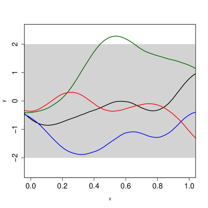
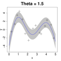
For our emulator the computer model’s output at all possible input vectors is modeled as a Gaussian stochastic process or random field, indexed by , expressing initial uncertainty about possible model results; several random draws from such a distribution are illustrated for a one-dimensional parameter space in Fig. 1(left). Emulator training is accomplished by evaluating the conditional probability distribution of model outputs at all input vectors , given observations of the actual computer model output at a finite collection of selected design input vectors . The emulator reproduces the model output perfectly at the design points, and offers predictive distributions for model output at other points which are more (or less) variable for points that are closer to (or further from) the design points, respectively. Although other distributions could be used for emulators, Gaussian processes (or GPs) are particularly convenient because the required conditional distributions can be computed very efficiently with simple matrix algebra.
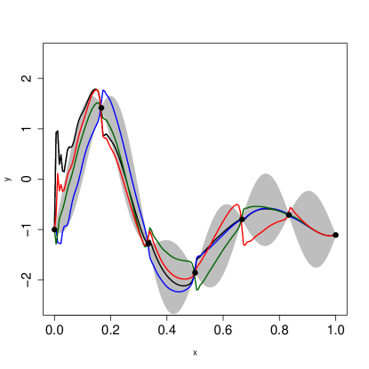
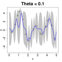
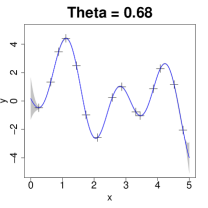
The detailed behaviour of the emulator is determined by the mean and covariance structure chosen for the GP and by the number and location of the training points. After removing simple linear effects with multiple regression and a possible nonlinear transformation of the computer model’s inputs and outputs, if necessary, the computer model may be assumed to be locally smooth (so small changes in lead to small changes in the output) and homogeneous (so the magnitude of predictive uncertainty is relatively constant). Under these assumptions the conventional mean-zero isotropic Gaussian random fields used in geostatistics [32, 33] work well; we used the commonly-recommended power exponential family [34, 35], with power close to its upper limit of two to ensure smoothness, and with correlation lengths fit to the data using maximum likelihood methods (emulator dependence on this parameter is illustrated in Fig. 2). A modest number of training points, perhaps 10–15 points per dimension in the parameter space, evenly distributed over the parameter range of interest will suffice. We used a Latin hypercube design, a space-filling approach which has proven very successful for all-purpose designs of computer experiment runs because it can “fill” the design space with very few points (see [35] or [36, Chap. 5]).
 |
 |
 |
To emulate functional output, when the computer model output for each input vector is not a single numerical quantity but a function of one or more variables, such as rapidity distributions or particle spectra which vary as a function of centrality, beam energy, etc…, we expand those functional outputs in an orthogonal basis (the most efficient choice is to use Principal Components), then construct independent Gaussian emulators as above for each component separately. This is only marginally more computationally demanding than the emulation of univariate computer model output.
In summary: emulators are computationally-trivial statistical approximations to functions that open exciting new doors for the statistical exploration of computationally-expensive models.
4 Initial State Variation
Let us now apply the emulator based on a Gaussian regression process to determine the initial state parameters from particle yields and spectra. By varying the Gaussian width that has been introduced in Section 2 the initial state granularity can be changed while keeping everything else constant. Fig. 3 (left) shows the result for transverse momentum spectra for pions and kaons in central Au+Au collisions at the highest RHIC energy. The slope of the spectra stays constant while the overall height which corresponds to the respective particle yield increases with increasing . This can be traced back to an increase in the total entropy of the initial state that is larger, if the particles are smeared out over a larger phase space volume.
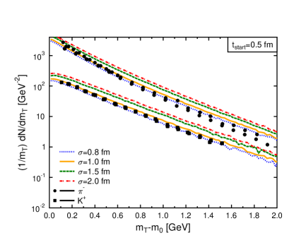
From earlier studies in [5] at lower energies it is known that the yields are also affected by the choice of the starting time. There is the possibility to compensate a change in by adjusting at the same time. Please note, that the starting time is here not only a way to normalize the initial state distributions as in hydrodynamic calculations with smooth initial conditions, but it is also the transition time from the hadronic transport approach to ideal hydrodynamics. By using the emulator to explore the two-dimensional parameter space in and , we can find parameter combinations that lead to the same pion yield/entropy in the system. The following parameter pairs can be identified and are listed in table 1.
| [fm] | 0.8 | 1.0 | 1.5 | 2.0 |
|---|---|---|---|---|
| [fm] | 0.3 | 0.5 | 1.2 | 1.8 |
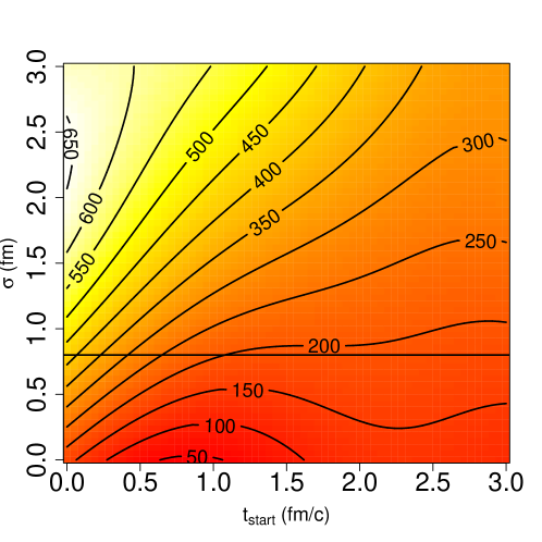
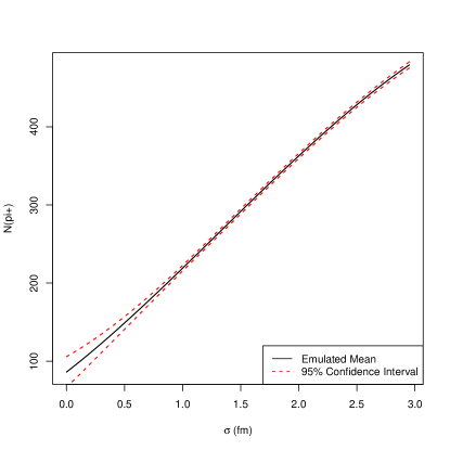
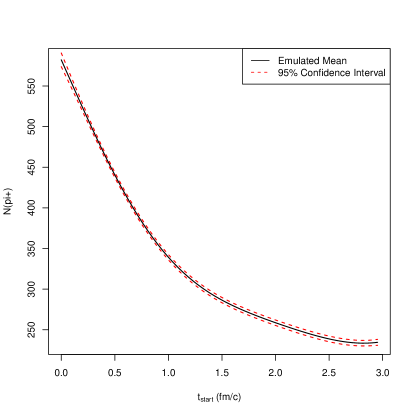
Fig. 4 shows the emulated mean number of pions produced in one collision as a function of the two initial state parameters and . A strong linear correlation between the parameters can be observed. The emulator was trained on 30 observations of the model distributed somewhat uniformly in the 2d parameter space. The variance of the emulator (Fig. 5) in the region where the simulation data was collected fm and fm is small, so we can be confident in the shape of the surface. The variance increases for fm which is a region of pure extrapolation, this is the expected behavior.
The linear correlation between start time and kernel width implies that more smearing in the initial state can be compensated for by prolonged evolution before the switch to hydrodynamical evolution.
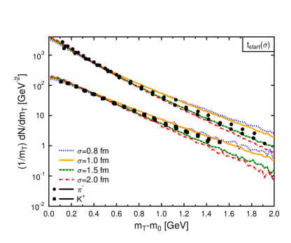
The result for the pion and kaon transverse momentum spectra for the four parameter combinations are shown in Fig. 3 (right). The particle yields are now kept constant, but the slope of the spectra is sensitive to the starting time. The earlier the starting time, the longer the duration of the hydrodynamic evolution, therefore there is more time to develop larger radial flow which leads to flatter transverse mass spectra. The difference in slope becomes clearly visible at higher values larger than 1 GeV.
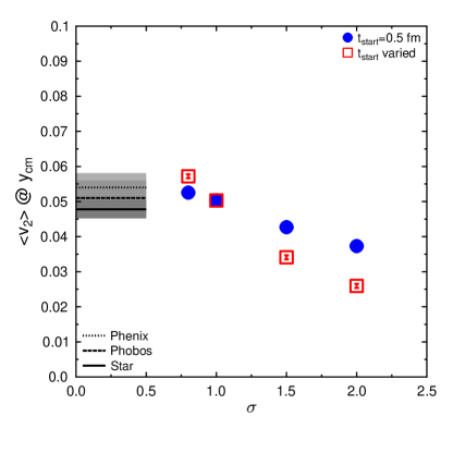
Let us now explore the influence of the different initial state parameters on the integrated elliptic flow in mid-central ( fm) Au+Au collisions at GeV. In Fig. 6 the averaged value of the second coefficient of the Fourier decomposition of the azimuthal distribution of charged particles in momentum space is shown as a function of the granularity . The filled circles represent the results for fixed starting time fm and the open squares show the result for the identified combinations in Table 1. Without changing the starting time the results for different granularities are compatible to the experimental data, that is indicated by the lines, even though the particle numbers are very different. The starting time can be constrained by looking at the spectra and elliptic flow to be less than 1 fm since later starting times do not allow for enough flow development during the hydrodynamic evolution. Just by looking at basic bulk observables like yields, spectra and integrated elliptic flow, we can constrain the initial state parameters within this approach to be around fm and fm which we will use as default in the following Section.
5 Fluctuating vs. Averaged Initial Conditions
Even though, we have shown in the last Section that the initial state parameters can be constrained by bulk observables, this does not necessarily constrain the granularity of the initial state. Previous studies at lower energies within the same hybrid approach have shown that there is some insensitivity to the event-by-event fluctuations of the initial state [43]. In contrast to the full event-by-event setup we have discussed so far, one can also look at calculations from averaged initial conditions. The default parameters are chosen to generate the initial state and one averages over 100 initial states from UrQMD to feed a smooth profile in the hydrodynamic calculation. This provides a different way to tune the initial state granularity between fluctuating (1 UrQMD event) to averaged smooth initial conditions (100 UrQMD events).
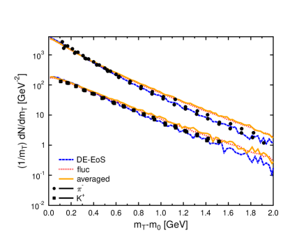
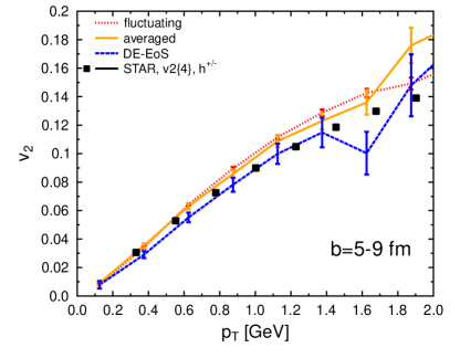
In Fig. 7 results for transverse mass spectra (left) and elliptic flow of pions as a function of transverse momentum (right) are shown for the fluctuating event-by-event setup and the averaged initial conditions. The results in this case are not affected since the analysis has been performed with respect to the reaction plane that is given by the coordinate system. Using the standard event plane method the elliptic flow results would be a little higher in the fluctuating case as has been shown in [45]. Furthermore, a softer equation of state based on a chiral hadronic Lagrangian that is coupled to the Polyakov loop including chiral symmetry restoration and a deconfinement phase transition that reproduces ground state properties and results from lattice QCD (DE-EoS) [46, 47, 48] has been applied to give an example of other ’parameters’ that may affect the results. As shown in Fig. 7 (left) the slope of the transverse mass spectra is smaller using the DE-EoS and leads to a better agreement with experimental data, while the elliptic flow result (right) is very similar. For the calculations with the other equation of state the freeze-out transition needs to be adjusted as well and a higher energy density criterion has been applied. A more detailed study of the freeze-out procedure is left for a future publication. At this point, it is mentioned as a further uncertainty.
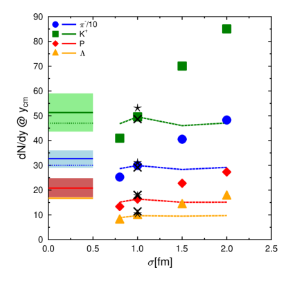
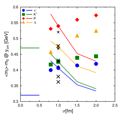
To wrap up the results of the present systematic study on initial state granularity and bulk observables in heavy ion reactions, in Fig. 8 results for yields and mean transverse momentum of pions, protons, kaons and ’ s are shown for all the 10 different cases that we have discussed in this paper so far. The full symbols represent the results where only has been changed while is fixed to be 0.5 fm. The multiplicities are proportional to the smearing parameter, whereas the radial flow is not as sensitive (with the exception of the ’s). By varying the starting time according to the result of the emulator (lines), we confirm that the yields can be kept constant but the mean transverse mass decreases significantly because of the later transition to the hydrodynamic evolution. One needs to start early enough to allow to develop radial flow and elliptic flow. From these two calculations the default parameters for and are constrained. Still one might vary the granularity by averaging over initial states instead of final states and the corresponding results are shown as stars. Bulk observables do not provide a good handle on the granularity since the results are very similar in the fluctuating and the averaged case. One needs to calculate fluctuation or correlation observables to really constrain the amount of initial state fluctuations. The equation of state including a deconfinement phase transition reduces the mean transverse masses to achieve a better agreement with the experimental data. We are not able to present a complete set of best fit parameters yet, since the freeze-out procedure needs to be improved before the statistical analysis is extended to include more parameters and more experimental data sets.
6 Summary and Conclusion
We have explored the capabilities of a novel statistical analysis utilizing Gaussian process emulators to address ambiguities in the initial state parameters used in a hybrid approach for the dynamical evolution of relativistic heavy ion reactions. The smearing parameter and the starting time of the hydrodynamic evolution are found to be correlated. By imposing a constant entropy constraint one finds viable combinations of these two parameters, which agree well with experimental data.
The comparison of the fluctuating event-by-event setup to averaged initial conditions using the same initial state parameters shows that bulk observables are insensitive to the initial state granularity. This insensitivity can be exploited in order to constrain quantities like e.g. the shear viscosity of QCD matter from averaged elliptic flow results. We note that significant sensitivities to the equation of state remain which can be utilized to constrain this input parameter. Our results show that state of the art statistical techniques for executing multi-parameter fits are required to reliably quantify properties of interest of hot and dense QCD matter. These techniques are now being developed and will lead us to achieve a better understanding of sensitivities on different parameter sets.
Acknowledgements
We are grateful to the Open Science Grid for the computing resources. The authors thank Dirk Rischke for providing the 1 fluid hydrodynamics code. H.P. acknowledges a Feodor Lynen fellowship of the Alexander von Humboldt foundation. This work was supported in part by U.S. department of Energy grant DE-FG02-05ER41367, NSF grants PHY-09-41373 and DMS-07-57549 and NASA grant NNX09AK60G.
References
References
- [1] S. A. Bass and A. Dumitru, Phys. Rev. C 61, 064909 (2000) [arXiv:nucl-th/0001033].
- [2] D. Teaney, J. Lauret and E. V. Shuryak, arXiv:nucl-th/0110037.
- [3] T. Hirano, U. W. Heinz, D. Kharzeev, R. Lacey and Y. Nara, Phys. Lett. B 636, 299 (2006) [arXiv:nucl-th/0511046].
- [4] C. Nonaka and S. A. Bass, Phys. Rev. C 75, 014902 (2007) [arXiv:nucl-th/0607018].
- [5] H. Petersen, J. Steinheimer, G. Burau, M. Bleicher and H. Stocker, Phys. Rev. C 78, 044901 (2008) [arXiv:0806.1695 [nucl-th]].
- [6] K. Werner, I. Karpenko, T. Pierog, M. Bleicher and K. Mikhailov, Phys. Rev. C 82, 044904 (2010) [arXiv:1004.0805 [nucl-th]].
- [7] H. Agakishiev et al., arXiv:1010.0690 [nucl-ex].
- [8] B. H. Alver, C. Gombeaud, M. Luzum and J. Y. Ollitrault, Phys. Rev. C 82, 034913 (2010) [arXiv:1007.5469 [nucl-th]].
- [9] B. Schenke, S. Jeon and C. Gale, arXiv:1009.3244 [hep-ph].
- [10] H. Petersen, G. Y. Qin, S. A. Bass and B. Muller, Phys. Rev. C 82, 041901 (2010) [arXiv:1008.0625 [nucl-th]].
- [11] G. Y. Qin, H. Petersen, S. A. Bass and B. Muller, arXiv:1009.1847 [nucl-th].
- [12] A. Mocsy and P. Sorensen, arXiv:1008.3381 [hep-ph].
- [13] S. A. Bass et al., Prog. Part. Nucl. Phys. 41, 255 (1998) [Prog. Part. Nucl. Phys. 41, 225 (1998)] [arXiv:nucl-th/9803035].
- [14] M. Bleicher et al., J. Phys. G 25, 1859 (1999) [arXiv:hep-ph/9909407].
- [15] B. Nilsson-Almqvist and E. Stenlund, Comput. Phys. Commun. 43, 387 (1987).
- [16] T. Sjostrand, Comput. Phys. Commun. 82, 74 (1994).
- [17] M. Bleicher et al., Nucl. Phys. A 638, 391 (1998).
- [18] F. Grassi, Y. Hama, O. Socolowski and T. Kodama, J. Phys. G 31, S1041 (2005).
- [19] R. Andrade, F. Grassi, Y. Hama, T. Kodama, O. . J. Socolowski and B. Tavares, Eur. Phys. J. A 29, 23 (2006) [arXiv:nucl-th/0511021].
- [20] R. Andrade, F. Grassi, Y. Hama, T. Kodama and O. . J. Socolowski, Phys. Rev. Lett. 97, 202302 (2006) [arXiv:nucl-th/0608067].
- [21] B. M. Tavares, H. J. Drescher and T. Kodama, Braz. J. Phys. 37, 41 (2007) [arXiv:hep-ph/0702224].
- [22] R. P. G. Andrade, F. Grassi, Y. Hama, T. Kodama and W. L. Qian, Phys. Rev. Lett. 101, 112301 (2008) [arXiv:0805.0018 [hep-ph]].
- [23] H. Petersen, T. Renk and S. A. Bass, arXiv:1008.3846 [nucl-th].
- [24] D. H. Rischke, S. Bernard and J. A. Maruhn, Nucl. Phys. A 595, 346 (1995) [arXiv:nucl-th/9504018].
- [25] D. H. Rischke, Y. Pursun and J. A. Maruhn, Nucl. Phys. A 595, 383 (1995) [Erratum-ibid. A 596, 717 (1996)] [arXiv:nucl-th/9504021].
- [26] H. Petersen, J. Steinheimer, M. Bleicher and H. Stocker, J. Phys. G 36, 055104 (2009) [arXiv:0902.4866 [nucl-th]].
- [27] Anthony O’Hagan, Reliability Engineering & System Safety, 91 (10-11):1290–1300, (2006), The Fourth International Conference on Sensitivity Analysis of Model Output (SAMO 2004) - SAMO 2004.
- [28] Jeremy E. Oakley and Anthony O’Hagan, Biometrika, 89 (4) :169-184, (2002).
- [29] Jeremy E. Oakley and Anthony O’Hagan, J. Roy. Stat. Soc. B,66,(2004).
- [30] M. J. Bayarri, James O. Berger, Rui Paulo, Jerome Sacks, John A. Cafeo, James C. Cavendish, Chin-Hsu Lin and Jian Tu, Technometrics, 49 (2):138-154, (2007).
- [31] David Higdon, James Gattiker, Brian Williams and Maria Rightley, J. Am. Stat. Assoc., 103 (482):570-583,(2008).
- [32] Jean-Paul Chilès and Pierre Delfiner, John Wiley & Sons, New York, NY, (1999).
- [33] Noel A. C. Cressie, John Wiley & Sons, New York, NY, (1993).
- [34] Marc C. Kennedy and Anthony O’Hagan, Biometrika, 87(1):1-13, (2000).
- [35] Jerome Sacks, William J. Welch, Toby J. Mitchell and Henry P. Wynn, Stat. Sci., 4 (4):409-435, November (1989).
- [36] Thomas J. Santner, Brian J. Williams and William Notz, Springer Series in Statistics, Springer-Verlag, New York, NY, (2003).
- [37] J. Adams et al. [STAR Collaboration], Phys. Rev. Lett. 92, 112301 (2004) [arXiv:nucl-ex/0310004].
- [38] S. S. Adler et al. [PHENIX Collaboration], Phys. Rev. C 69, 034909 (2004) [arXiv:nucl-ex/0307022].
- [39] I. Arsene et al. [BRAHMS Collaboration], Phys. Rev. C 72, 014908 (2005) [arXiv:nucl-ex/0503010].
- [40] S. Esumi [PHENIX Collaboration], Nucl. Phys. A 715, 599 (2003) [arXiv:nucl-ex/0210012].
- [41] S. Manly et al. [PHOBOS Collaboration], Nucl. Phys. A 715, 611 (2003) [arXiv:nucl-ex/0210036].
- [42] R. L. Ray [STAR Collaboration], Nucl. Phys. A 715, 45 (2003) [arXiv:nucl-ex/0211030].
- [43] H. Petersen and M. Bleicher, Phys. Rev. C 81, 044906 (2010) [arXiv:1002.1003 [nucl-th]].
- [44] B. I. Abelev et al. [STAR Collaboration], Phys. Rev. C 77, 054901 (2008) [arXiv:0801.3466 [nucl-ex]].
- [45] H. Holopainen, H. Niemi and K. J. Eskola, arXiv:1007.0368 [hep-ph].
- [46] J. Steinheimer, V. Dexheimer, H. Petersen, M. Bleicher, S. Schramm and H. Stoecker, Phys. Rev. C 81, 044913 (2010) [arXiv:0905.3099 [hep-ph]].
- [47] J. Steinheimer, S. Schramm and H. Stocker, arXiv:0909.4421 [hep-ph].
- [48] S. Borsanyi, G. Endrodi, Z. Fodor et al., JHEP 1011 (2010) 077 [arXiv:1007.2580 [hep-lat]].
- [49] D. Ouerdane [BRAHMS Collaboration], Nucl. Phys. A 715, 478 (2003) [arXiv:nucl-ex/0212001].
- [50] J. H. Lee et al. [BRAHMS Collaboration], J. Phys. G 30, S85 (2004).
- [51] J. Adams et al. [STAR Collaboration], Phys. Rev. Lett. 98, 062301 (2007) [arXiv:nucl-ex/0606014].