Fitness-driven deactivation in network evolution

Abstract

Individual nodes in evolving real-world networks typically experience growth and decay — that is, the popularity and influence of individuals peaks and then fades. In this paper, we study this phenomenon via an intrinsic nodal fitness function and an intuitive aging mechanism. Each node of the network is endowed with a fitness which represents its activity. All the nodes have two discrete stages: active and inactive. The evolution of the network combines the addition of new active nodes randomly connected to existing active ones and the deactivation of old active nodes with possibility inversely proportional to their fitnesses. We obtain a structured exponential network when the fitness distribution of the individuals is homogeneous and a structured scale-free network with heterogeneous fitness distributions. Furthermore, we recover two universal scaling laws of the clustering coefficient for both cases, $C(k)\sim k^{-1}$ and $C\sim n^{-1}$, where $k$ and $n$ refer to the node degree and the number of active individuals, respectively. These results offer a new simple description of the growth and aging of networks where intrinsic features of individual nodes drive their popularity, and hence degree.

Keywords: random graphs, networks, fitness, power law

1 Introduction

Over the past decade, there has been an explosion of interest in complex networks for describing structures and dynamics of complex systems. Despite differences in their nature, many networks may be characterized by similar topological properties. For instance, real networks display highly clustering than expected from classic random graphs [1]. Also, it has been widely observed that node-degree distributions of many large networks are heavy tailed [2], e.g., exponential and power-law. To understand how these phenomena arise, research devoted to evolving networks has rapidly flourished [3, 4, 5, 6, 7, 8]. The basic premise is that the network will continue to grow at a constant rate and new nodes attach to old ones with some possibility. When the newly added nodes connect with equal probability to nodes already present in the network, the degree distribution of the nodes of the resulting network is exponential. Whereas for newcomers connecting to old ones with linear preference of the node degree, Barabási and Albert (BA) observed a power-law distribution of connectivity [3].

In the real world, agents, represented by nodes, always age after growth. For instance, in scientific citation networks there is a half-life effect: old papers are rarely cited since they are no longer sufficiently topical (or they are more often referenced through secondary literature). On the World Wide Web popular web sites (for example, search engines) will often loose favor to newer alternatives. To study the effect of this phenomenon on network evolution, the BA model has been modified by incorporating time dependence in the network [9, 10, 11, 12, 13, 14, 15, 16, 17, 18, 19]. Dorogovtsev and Mendes studied the case when the connection probability of the new node with an old one is not only proportional to the degree $k$ but also to a power of its present age $\tau^{-\alpha}$ (where $\tau$ is the age of a node) [9]. They found that the network shows scale-free (SF) behavior only in the region $\alpha<1$. For $\alpha>1$, the distribution $P(k)$ is exponential. Yet, the gradual aging model show lower clustering than realistic networks. On the contrary, Klemm and Eguíluz considered evolving networks based on the memory of nodes and proposed a degree-dependent deactivation network model [15] which is highly clustered and retains the power-law distribution of the degree (but no consideration of exponential degree distributions).

The aim of this paper is to propose a simpler and more fundamental mechanism to build networks, including SF networks, while retaining the positive features of aforesaid models. The mechanism we propose simulates realistic networks, and can be understood analytically. It has been shown that in some networks, the popularity (or activity) of a node is essentially determined by the so-called “fitness”[20, 21, 22, 23] which is intrinsically related to the role played by each node, such as the innovation of a scientific paper or the content of a webpage. This allows us to represent the activities of individuals by intrinsic fitnesses and suggest a fitness-driven deactivation approach to build structured networks. Compared with topological information, the intrinsic fitness provides a more natural and appropriate deactivation criterion for aging of nodes. We show that depending on the node-fitness distributions two topologically different networks can emerge, the connectivity distribution following either an exponential or a generalized power law. In both cases, the networks are highly clustered. Irrespective of the fitness distribution, we observe two scaling laws of the clustering coefficient, $C(k)\sim k^{-1}$ and $C\sim n^{-1}$, where $k$ is the node degree and $n$ corresponds to the number of active individuals in the network. Hence, this mechanism offers an explanation for the origin and ubiquity of such clustering in real networks.

2 Model

Rather than connectivity-dependent deactivation dynamics of the nodes developed in [15, 16, 17, 18, 19], the present deactivation model is based on the individual fitnesses. For each node $i$ a fitness $x_{i}>0$, the random number drawn from a given probability distribution function $\rho(x)$, is assigned to measure its popularity or activity. The deactivation mechanism is characterized by the transition of a node from the active to the inactive state interpreted as a collective forgetting of it.

The network starts from an initial seed of $n$ nodes, totally connected by undirect edges, which are all active. Then at each time step the dynamics runs as follows.

(i) Add a new node $i$, which connects to $m$ ($m\leq n$) nodes randomly chosen from the $n$ active ones. By $k^{{\rm in}}$ we denote the in-degree of a node, i.e., the number of edges pointing to it. The in-degree of the newcomer is $k_{i}^{\rm{in}}=0$ at first. Each selected active node $j$ receives exactly one incoming edge, thereby $k_{j}^{\rm{in}}\rightarrow k_{j}^{\rm{in}}+1$. Since the out-degree of each node is $m$ always, the total degree of a node is $k=k^{\rm{in}}+m$.

(ii) Activate the new node and deactivate one (denoted by $j$) of the $n$ old active nodes with probability

$$\pi(x_{j})=\sigma x_{j}^{-1},$$ (1)

where $\sigma=(\sum_{j\in{\rm\Lambda}}x_{j}^{-1})^{-1}$ is the normalization factor. The summation runs over the set $\Lambda$ of the $n$ old active nodes.

During evolution, a node might receive edges while it is active, and once inactive it will not receive edges any more. Note that the fitter the individual is, the more difficult for it to be deactivated. For the case of the citation network, Eq. (1) means that the famous paper with great innovation is less possibility to be forgotten.

3 Degree distribution

Denoting by $a(k,x,t)$ the probability of active nodes with degree $k$ and fitness $x$ at time $t$, we can write out the master equation for network evolution

$$a(k+1,x,t+1)=a(k+1,x,t)[1-\pi(x)](1-\frac{m}{n})+a(k,x,t)[1-\pi(x)]\frac{m}{n}.$$ (2)

At each time step, an active node is deactivated and a newcomer joins the set $\Lambda$ to keep the number $n$ unchanged. According to Eq. (1), the normalization factor $\sigma$ varies with time because of the change of the nodes in the active set. However, the fitness of each node is a random number taken from a given probability distribution $\rho(x)$, therefore the normalization $\sigma$ fluctuates very slightly and can be treated as a constant. Substituting Eq. (1) into Eq. (2) yields

$$a(k+1,x,t+1)\approx a(k+1,x,t)(1-\frac{\sigma}{x})(1-\frac{m}{n})+a(k,x,t)(1-\frac{\sigma}{x})\frac{m}{n}.$$ (3)

Imposing the stationarity condition $a(k,x,t)=a(k,x)$, we obtain the equation

$$a(k+1,x)=\frac{m(x-\sigma)}{m(x-\sigma)+n\sigma}a(k,x)=\left[\frac{m(x-\sigma)}{m(x-\sigma)+n\sigma}\right]^{k-m}a(m,x)$$ (4)

for the probability of active nodes with degree $k+1$ and fitness $x$ in the stationary state, where

$$a(m,x)=\frac{n(x-\sigma)}{m(x-\sigma)+n\sigma}\rho(x)$$ (5)

is the stationary probability of active nodes with degree $m$ and fitness $x$. Then we obtain

$$a(k,x)=\frac{n}{m}\left[\frac{m(x-\sigma)}{m(x-\sigma)+n\sigma}\right]^{k-m}\rho(x).$$ (6)

Denoting by $a(k)$ the possibility of active nodes with degree $k$ in the steady state, we have

$$a(k)=\int_{0}^{x_{{\rm max}}}a(k,x){\rm d}x=\int_{0}^{x_{{\rm max}}}\frac{n}{m}\left[\frac{m(x-\sigma)}{m(x-\sigma)+n\sigma}\right]^{k-m}\rho(x)\rm{d}x.$$ (7)

In case the total number $N$ of nodes in the network is larger than the number $n$ of active nodes, the degree distribution $P(k)$ can be approximated by considering inactive nodes only. Thus, $P(k)$ can be calculated as the rate of the change of $a(k)$,

$$P(k) = -\frac{{\rm d}a(k)}{{\rm d}k}$$ (8)

$$= \int_{0}^{x_{{\rm max}}}\frac{n}{m}\left[\frac{m(x-\sigma)}{m(x-\sigma)+n\sigma}\right]^{k-m}\ln\left[\frac{m(x-\sigma)}{m(x-\sigma)+n\sigma}\right]^{-1}\rho(x){\rm d}x.$$

Even when the form of $\rho(x)$ is given, it is still difficult to solve the integral on the right-hand side of the equation. Instead, we need a more subtle technique. We assume that

$$F(x) = \frac{m(x-\sigma)}{m(x-\sigma)+n\sigma},$$ (9)

$$G(x) = \frac{n}{m}[F(x)]^{-m}\ln[F(x)]^{-1}\rho(x).$$ (10)

Without lack of generality, we also normalize the fitnesses. Now Eq. (8) can be rewritten as

$$P(k)=\int_{0}^{1}[F(x)]^{k}G(x){\rm d}x.$$ (11)

As will be seen below, for the proper choice of $F$ and $G$, one can construct networks with exponential or power-law degree distributions, and then determine the forms of the corresponding fitness distributions.

(i) Exponential degree distribution. We set $F(x)=1/\mu$ and $G(x)=\nu$, where $\mu(>1)$ and $\nu$ are positive constants. Consequently, the integral of Eq. (11) is

$$P(k)=\nu\mu^{-k},$$ (12)

following an exponential. According to the definition of $F(x)$, we have

$$\frac{m(x-\sigma)}{m(x-\sigma)+n\sigma}=\frac{1}{\mu},$$ (13)

the solution of which reads

$$x=\sigma+\frac{n\sigma}{m(\mu-1)}={\rm constant}.$$ (14)

Then the normalization factor becomes

$$\sigma=\left\{n\left[\sigma+\frac{n\sigma}{m(\mu-1)}\right]^{-1}\right\}^{-1},$$ (15)

yielding

$$\mu=1+\frac{n}{m(n-1)}.$$ (16)

According to the definition of $G(x)$, we have

$$\nu=\frac{n}{m}\mu^{m}\ln\mu\rho(x),$$ (17)

which suggests

$$\rho(x)=\frac{m\nu}{n\mu^{m}\ln\mu}={\rm constant}.$$ (18)

According to the normalization, $\rho(x)$ should satisfy $\int_{0}^{1}\rho(x){\rm d}x=1$. Combining Eqs. (14) and (18), we finally obtain the distribution of $\rho(x)$,

$$\rho(x)=\delta\left(x-\frac{\sigma(m\mu-m+n)}{m(\mu-1)}\right).$$ (19)

That is to say, the fitness of each node is identical. Considering the constant approximation of $\sigma$, the above result can be generalized to homogeneous distributions of fitnesses. Here, homogeneity implies that the node fitnesses have small fluctuations around the mean $\langle x\rangle$, hence the small variance. We conclude that for any given $\rho(x)$ distributing homogeneously, the fitness-driven deactivation generates structured exponential networks.

(ii) Power-law degree distribution. We set $F(x)=e^{-\phi x}$ and $G(x)=\varphi x^{\gamma}$, where $\phi$, $\varphi$ and $\gamma$ are positive constants. Accordingly, Eq. (11) can be rewritten as

$$P(k)=\frac{\varphi}{(\phi k)^{\gamma+1}}\int_{0}^{\phi k}e^{-z}z^{\gamma}{\rm d}z.$$ (20)

In the limit $k\rightarrow\infty$, one has $\int_{0}^{\phi k}e^{-z}z^{\gamma}{\rm d}z=\Gamma(\gamma+1)$. For any finite $k$, the integral $\int_{0}^{\phi k}e^{-z}z^{\gamma}{\rm d}z$ is convergent and smaller than $\Gamma(\gamma+1)$. Thus the connectivity distribution has a power-law form

$$P(k)\sim k^{-\gamma-1}.$$ (21)

Combining Eqs. (9) and (10), we obtain

$$\rho(x)=\frac{\varphi m}{\phi n}x^{\gamma-1}e^{-\phi mx}.$$ (22)

This heavy tailed distribution implies large fluctuations of the node fitnesses, hence heterogeneity. We conclude that the fitness-driven deactivation can build structured SF networks if the node fitnesses are distributed heterogeneously.

Figure 1: (Color online) Degree distributions of nodes of generated networks for different fitness distribution functions: uniform (a), Gaussian (b), exponential $e^{-x}$ (c), and power-law $x^{-1}$ (d). All the fitnesses have been normalized. For uniform and Gaussian distributions with the same mean ($0.5$) and small variances ($0.08(4)$ and $0.01(6)$), the node fitnesses fluctuate slightly around the mean and can be regarded as the homogeneity; whereas for exponential and power-law distributions, there are large fluctuations of the node fitnesses due to the right-skewed feature, resulting in the heterogeneity. The experiment networks start from the initial $n=10$ nodes and end with the total population $N=10^{5}$.

Figure 2: (Color online) The dependence of the slopes of the lines in Fig. 1 on $m$. In the inset, the data reported on the log-log representation show a power law $m^{-\xi}$, and the best linear fit gives $\xi=0.98(1)$.

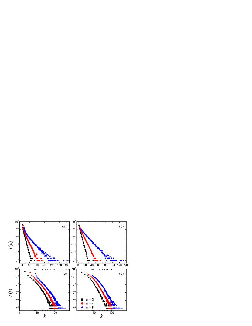
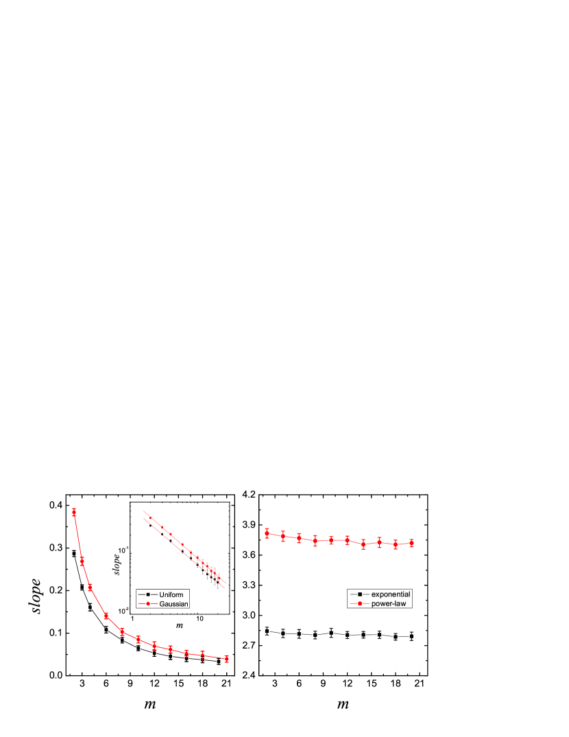
In Fig. 1 we give the simulation results of degree distributions $P(k)$ for four kinds of distribution functions $\rho(x)$ of node fitnesses. In case that the distributions of fitnesses are homogeneous, e.g., uniform (Fig. 1(a)) and Gaussian (Fig. 1(b)), the linear-log plots imply an exponential degree distribution. Conversely, when the fitnesses distribute heterogeneously, the log-log plots of Figs. 1(c) and 1(d), corresponding to exponential and power-law cases respectively, predict a generalized power law. We obtain the slopes of the lines in Fig. 1 by least squares fitting and plot them as a function of $m$ in Fig. 2. For homogeneous fitnesses, we notice a scaling relation between the slope and $m$, whereas for heterogenous fitnesses, the slope shows independence on $m$.

4 Clustering coefficient

In a network, if a node $i$ has $k_{i}$ edges, and among its $k_{i}$ nearest neighbors there are $e_{i}$ edges, then the clustering coefficient of $i$ is defined by

$$c_{i}=\frac{2e_{i}}{k_{i}(k_{i}-1)}.$$ (23)

In the deactivation model, new edges are created between the selected active nodes and the added one. Let us first consider the case of $n=m$. At each time step, the degree $k_{i}$ of the active node $i$ increases by $1$ and $e_{i}$ increase by $m-1$ until it is deactivated. Therefore, the evolutionary dynamics of $k_{i}$ and $e_{i}$ are given by

$$k_{i} = (m+t),$$ (24)

$$\frac{de_{i}}{dt} = (m-1).$$ (25)

Integrating Eq. (25) with the boundary condition $e_{i}(0)=m(m-1)/2$ and substituting the solution into Eq. (23), we recover the clustering coefficient $c(k)$ restricted to the nodes of degree $k$ [16, 17]

$$c(k)=\frac{2(m-1)}{k-1}-\frac{m(m-1)}{k(k-1)}.$$ (26)

For $n>m$, the clustering coefficient $C(k)$ is just the generalization of Eq. (26),

$$C(k)=\frac{m}{n}\left[\frac{2(m-1)}{k-1}-\frac{m(m-1)}{k(k-1)}\right],$$ (27)

which indicates that the local clustering scales as $C(k)\sim k^{-1}$ for large $k$. The clustering coefficient $C$ of the whole network is the mean of $C(k)$ with respect to the degree distribution $P(k)$,

$$C=\int_{m}^{\infty}C(k)P(k){\rm d}k.$$ (28)

Substituting Eqs. (12) and (21) into the integral respectively, we obtain

$$C\sim\left\{\begin{array}[]{lll}&\frac{2\nu(m^{2}-m)}{n}\int_{m}^{\infty}\frac{\mu^{-k}}{k}{\rm d}k+\frac{\nu(m^{2}-m^{3})}{n}\int_{m}^{\infty}\frac{\mu^{-k}}{k(k-1)}{\rm d}k,\\ &\frac{2(m^{2}-m)}{n}\int_{m}^{\infty}\frac{{\rm d}k}{k^{\gamma+2}}+\frac{(m^{2}-m^{3})}{n}\int_{m}^{\infty}\frac{{\rm d}k}{k^{\gamma+2}(k-1)},\\ \end{array}\right.$$ (29)

proportional to $n^{-1}$.

Figure 3: (Color online) Log-log plots of $C(k)$ as a function of $k$ for different fitness distribution functions: uniform (a), Gaussian (b), exponential $e^{-x}$ (c), and power-law $x^{-1}$ (d). The solid lines correspond to a power law $2k^{-1}$.

Figure 4: (Color online) Log-log plots of $C$ as a function of $n$ for different fitness distribution functions: uniform (a), Gaussian (b), exponential $e^{-x}$ (c), and power-law $x^{-1}$ (d). The solid lines correspond to a power law $2n^{-1}$.

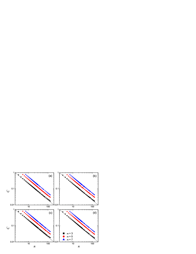
In Fig. 3 we show the simulation results of $C(k)$ as a function of $k$. All the plots follow a power law $C(k)\sim k^{-1}$, which coincides with the expression in Eq. (27). For the clustering coefficient of the whole network, as shown in Fig. 4, the linearity of all the plots also implies a power-law relation $C\sim n^{-1}$. It is worth noting that both the scaling laws are independent of fitness distribution functions. One obtains the same result for uniform, Gaussian, exponential and power-law distributions of fitnesses.

5 Conclusion

In this paper, we have presented an alternatively simple and intuitive model for a large and important class of networks widely observed in the real world. We defined the intrinsic fitness as the way of quantifying the popularity of individuals, i.e., the fitter a node is, the higher possibility it is active. The growth dynamics of the network is governed by the naive fitness-driven deactivation mechanism. The deactivation probability of a node is proportional to the inverse of its fitness, which characterizes the individual capability of obtaining further links. We studied the connectivity distribution and the clustering coefficient that can fundamentally shape a network. On one hand, we found the great influence of the node fitnesses on the connectivity distribution. The homogeneous fitnesses generate exponential networks, while the heterogeneous fitnesses result in SF ones. On the other hand, we recovered two universal scaling laws of the clustering coefficient regardless of the fitness distributions. These results are consistent with what has been empirically observed in many real-world networks in (for example) [24, 25, 26, 27], and so the present model provides a new way to understand complex networks with age.

References

- [1] Watts D J, 1999 Small Worlds: The Dynamics of Networks Between Order and Randomness (New Jersey: Princeton University Press)
- [2] Amaral L A N, Scala A, Barthélemy M and Stanley H E, 2000 Proc. Natl. Acad. Sci. U.S.A. 97 11149
- [3] Barabási A L and Albert R, 1999 Science 286 509
- [4] Krapivsky P L, Redner S and Leyvraz F, 2000 Phys. Rev. Lett. 85 4629
- [5] Dorogovtsev S N, Mendes J F F and Samukhin A N, 2000 Phys. Rev. Lett. 85 4633
- [6] Albert R and Barabási A L, 2000 Phys. Rev. Lett. 85 5234
- [7] Dorogovtsev S N and Mendes J F F, 2001 Phys. Rev. E 63 056125
- [8] Krapivsky P L and Redner S, 2001 Phys. Rev. E 63 066123
- [9] Dorogovtsev S N and Mendes J F F, 2000 Phys. Rev. E 62 1842
- [10] Zhu H, Wang X R and Zhu J Y, 2003 Phys. Rev. E 68 056121
- [11] Hajra K B and Sen P, 2004 Phys. Rev. E 70 056103
- [12] Herdaǧdelen A, Aygün E and Bingol H, 2007 Europhys. Lett. 78 60007
- [13] Lambiotte R, 2007 J. Stat. Mech. P02020
- [14] Crokidakis N and de Menezes M A, 2009 J. Stat. Mech. P04018
- [15] Klemm K and Eguíluz V M, 2002 Phys. Rev. E 65 036123
- [16] Klemm K and Eguíluz V M, 2002 Phys. Rev. E 65 057102
- [17] Vázquez A, Boguñá M, Moreno Y, Pastor-Satorras R and Vespignani A, 2003 Phys. Rev. E 67 046111
- [18] Wu Z X, Xu X J and Wang Y H, 2005 Phys. Rev. E 71 066124
- [19] Tian L, Zhu C P, Shi D N, Gu Z M and Zhou T, 2006 Phys. Rev. E 74 046103
- [20] Bianconi G and Barabási A L, 2001 Europhys. Lett. 54 436
- [21] Caldarelli G, Capocci A, Rios P D L and Muñoz M A, 2002 Phys. Rev. Lett. 89 258702
- [22] Garlaschelli D and Loffredo M I, 2004 Phys. Rev. Lett. 93 188701
- [23] Servedio V D P and Caldarelli G, 2004 Phys. Rev. E 70 056126
- [24] Williams R J and Martinez N D, 2000 Nature 404 180
- [25] Newman M E J, 2001 Proc. Natl. Acad. Sci. U.S.A. 98 404
- [26] Ravasz E and Barabási A L, 2003 Phys. Rev. E 67 026112
- [27] Börner K, Maru J T and Goldstone R L, 2004 Proc. Natl. Acad. Sci. U.S.A. 101 5266