A CLOSED FORMULA FOR THE BARRIER TRANSMISSION COEFFICIENT IN QUATERNIONIC QUANTUM MECHANICS

Abstract

In this paper, we analyze, by using a matrix approach, the dynamics of a non-relativistic particle in presence of a quaternionic potential barrier. The matrix method used to solve the quaternionic Schr dinger equation allows to obtain a closed formula for the transmission coefficient. Up to now, in quaternionic quantum mechanics, almost every discussion on the dynamics of non-relativistic particle was motived by or evolved from numerical studies. A closed formula for the transmission coefficient stimulates an analysis of qualitative differences between complex and quaternionic quantum mechanics, and, by using the stationary phase method, gives the possibility to discuss transmission times.

02.30.Tb, 03.65.Ca (PACS).

I. INTRODUCTION

In the quaternionic formulation of non-relativistic quantum mechanics, the dynamics of a particle without spin subject to the influence of the anti-hermitian scalar potential,

$$i\,V_{\mbox{\tiny$1$}}(\boldsymbol{r},t)+j\,V_{\mbox{\tiny$2$}}(\boldsymbol{r},t)+k\,V_{\mbox{\tiny$3$}}(\boldsymbol{r},t)\,\,,$$

is described by

$$\hbar\,\partial_{t}\Psi(\boldsymbol{r},t)=\left[\,i\,\frac{\,\,\hbar^{{}^{2}}}{2m}\,\nabla^{{}^{2}}-i\,V_{\mbox{\tiny$1$}}(\boldsymbol{r},t)-j\,V_{\mbox{\tiny$2$}}(\boldsymbol{r},t)-k\,V_{\mbox{\tiny$3$}}(\boldsymbol{r},t)\,\right]\,\Psi(\boldsymbol{r},t)~{}.$$ (1)

Eq.(1) is known as the quaternionic Schrödinger equation. For a detailed discussion on foundations of quaternionic quantum mechanics, we refer the reader to Adler’s book[1]. Numerical investigations on the observability of quaternionic deviations from the standard (complex) quantum mechanics[2, 3, 4, 5, 6, 7, 8, 9, 10] have recently stimulated the study of new mathematical tools in solving quaternionic differential equations[11, 12, 13, 14, 15, 16].

In complex quantum mechanics[17, 18], the rapid spatial variations of a square potential introduce purely quantum effects in the motion of the particle. Before beginning our analytic study of the quaternionic potential barrier and analyze analogies and differences between the complex and quaternionic dynamics, we introduce some important mathematical properties of the quaternionic Schrödinger equation in the presence of time independent potentials,

$$\hbar\,\partial_{t}\Psi(\boldsymbol{r},t)=\left[\,i\,\frac{\,\,\hbar^{{}^{2}}}{2m}\,\nabla^{{}^{2}}-i\,V_{\mbox{\tiny$1$}}(\boldsymbol{r})-j\,V_{\mbox{\tiny$2$}}(\boldsymbol{r})-k\,V_{\mbox{\tiny$3$}}(\boldsymbol{r})\,\right]\,\Psi(\boldsymbol{r},t)~{}.$$ (2)

Due to the fact that our analysis is done for a time independent potential, we can apply the method of separation of variables. So, we introduce

$$\Psi(\boldsymbol{r},t)=\Phi(\boldsymbol{r})\,\exp[\,-\,\mbox{$\frac{i}{\hbar}$}\,E\,t\,]\,\,.$$ (3)

The position on the right of the complex exponential is important to factorize the time dependent function. Then, Eq.(2) reduces to the following quaternionic (right complex linear) ordinary differential equation[12]

$$-\,E\,\Phi(\boldsymbol{r})\,i=\left[\,i\,\frac{\,\,\hbar^{{}^{2}}}{2m}\,\nabla^{{}^{2}}-i\,V_{\mbox{\tiny$1$}}(\boldsymbol{r})-j\,V_{\mbox{\tiny$2$}}(\boldsymbol{r})-k\,V_{\mbox{\tiny$3$}}(\boldsymbol{r})\,\right]\,\Phi(\boldsymbol{r})~{}.$$ (4)

In the case of a one-dimensional potential, $\boldsymbol{V}(\boldsymbol{r})=\boldsymbol{V}(x)$, and for a particle moving in the $x$-direction, $\Phi(\boldsymbol{r})=\Phi(x)$, the previous equation becomes

$$-\,E\,\Phi(x)\,i=\left[\,i\,\frac{\,\,\hbar^{{}^{2}}}{2m}\,\partial_{xx}-i\,V_{\mbox{\tiny$1$}}(x)-j\,V_{\mbox{\tiny$2$}}(x)-k\,V_{\mbox{\tiny$3$}}(x)\,\right]\,\Phi(x)~{}.$$ (5)

In the case of a quaternionic barrier,

$$\boldsymbol{V}(x)=\left\{\,\mbox{zone I}:\,\,\boldsymbol{0}\,\,\,(x<0)\,\,,\,\,\,\,\,\mbox{zone II}:\,\,\boldsymbol{V}\,\,\,(0<x<L)\,\,,\,\,\,\,\,\mbox{zone III}:\,\,\boldsymbol{0}\,\,\,(x>L)\,\right\}\,\,,$$

the plane wave solution is obtained by solving a second order differential equations with (left) constant quaternionic coefficients[12, 16]. To shorten our notation, it is convenient to rewrite the quaternionic differential equation (5) in terms of adimensional quantities. In the potential region, $0<\xi<\lambda$, the differential equation to be solved is

$$i\,\Phi_{\mbox{\tiny II}}^{\prime\prime}(\xi)=i\,V_{c}\,\Phi_{\mbox{\tiny II}}(\xi)+j\,V_{q}\,e^{-i\theta}\,\Phi_{\mbox{\tiny II}}(\xi)-\epsilon^{\mbox{\tiny$2$}}\,\Phi_{\mbox{\tiny II}}(\xi)\,i\,\,,$$ (6)

where

$$\epsilon=\sqrt{E/V_{\mbox{\tiny$0$}}}\,\,,\,\,\,V_{\mbox{\tiny$0$}}=\sqrt{V_{\mbox{\tiny$1$}}^{{}^{\mbox{\tiny$2$}}}+V_{\mbox{\tiny$2$}}^{{}^{2}}+V_{\mbox{\tiny$3$}}^{{}^{2}}}\,\,,\,\,\,V_{c}=V_{\mbox{\tiny$1$}}/V_{\mbox{\tiny$0$}}\,\,,\,\,\,V_{q}=\sqrt{V_{\mbox{\tiny$2$}}^{{}^{2}}+V_{\mbox{\tiny$3$}}^{{}^{2}}}/V_{\mbox{\tiny$0$}}\,\,,\,\,\,\arctan\theta=V_{\mbox{\tiny$3$}}/V_{\mbox{\tiny$2$}}\,\,,$$

and

$$\xi=\sqrt{2m\,V_{\mbox{\tiny$0$}}/\hbar^{{}^{2}}}\,\,x\,\,,\,\,\,\,\,\lambda=\sqrt{2m\,V_{\mbox{\tiny$0$}}/\hbar^{{}^{2}}}\,\,L\,\,.$$

The general solution contains four complex coefficients ($A$, $\widetilde{A}$, $B$, and $\widetilde{B}$) to be determined by the boundary conditions,

$$\Phi_{\mbox{\tiny II}}(\xi)=(1+j\,\gamma)\,\left\{\exp\left[\,\alpha_{\mbox{\tiny$-$}}\,\xi\,\right]\,A+\exp\left[\,-\,\alpha_{\mbox{\tiny$-$}}\,\xi\,\right]\,B\right\}+(\beta+j)\,\left\{\exp\left[\,\alpha_{\mbox{\tiny$+$}}\,\xi\,\right]\,\widetilde{A}+\exp\left[\,-\,\alpha_{\mbox{\tiny$+$}}\,\xi\,\right]\,\widetilde{B}\right\}\,\,,$$ (7)

for a detailed derivation of this solution see ref.[16]. The potential and energy inputs appear in the following complex quantities

$$\alpha_{\mbox{\tiny$\pm$}}=\sqrt{V_{c}\pm\sqrt{\epsilon^{\mbox{\tiny$4$}}-V_{q}^{{}^{2}}}}\,\,\,,\,\,\,\,\,\beta=i\,\frac{V_{q}\,e^{i\theta}}{\epsilon^{\mbox{\tiny$2$}}+\sqrt{\epsilon^{\mbox{\tiny$4$}}-V_{q}^{{}^{2}}}}\,\,\,,\,\,\,\,\,\gamma=-\,i\,\frac{V_{q}\,e^{-i\theta}}{\epsilon^{\mbox{\tiny$2$}}+\sqrt{\epsilon^{\mbox{\tiny$4$}}-V_{q}^{{}^{2}}}}\,\,\,.$$ (8)

Note that for $E\geq\sqrt{V_{\mbox{\tiny$2$}}^{{}^{2}}+V_{\mbox{\tiny$3$}}^{{}^{2}}}$, we have $\gamma=\beta^{*}$.

In the free potential regions, zone I ($\xi<0$) and zone III ($\xi>\lambda$), the solutions are given by

$$\begin{array}[]{lcl}\Phi_{\mbox{\tiny I}}(\xi)&=&\exp\left[\,i\,\epsilon\,\xi\,\right]+\exp\left[\,-\,i\,\epsilon\,\xi\,\right]\,R+j\,\exp\left[\,\epsilon\,\xi\,\right]\,\widetilde{R}\,\,,\\ \Phi_{\mbox{\tiny III}}(\xi)&=&\exp\left[\,i\,\epsilon\,\xi\,\right]\,T+j\,\exp\left[\,-\,\epsilon\,\xi\,\right]\,\widetilde{T}\,\,.\end{array}$$ (9)

It is important to observe that starting from theses solutions we can find the relation between reflection and transmission coefficients without the necessity to know their explicit formulas. In fact, for stationary states the density probability is independent from the time and, consequently, the current density $\Phi^{{\dagger}}(x)\,i\,\Phi^{\prime}(x)+\mbox{h.c.}$ is a constant in $x$. This implies, for example,

$$\Phi_{\mbox{\tiny I}}^{{\dagger}}(0)\,i\,\Phi_{\mbox{\tiny I}}^{\prime}(0)+\mbox{h.c.}=\Phi_{\mbox{\tiny III}}^{{\dagger}}(\lambda)\,i\,\Phi_{\mbox{\tiny III}}^{\prime}(\lambda)+\mbox{h.c.}\,\,.$$

From this relation, we get the well known norm conservation formula, i.e.

$$1-|R|^{{}^{2}}=|T|^{{}^{\mbox{\tiny$2$}}}\,\,.$$ (10)

Having introduced this preliminary discussion on the quaternionic Schrödinger equation, we can now return to our task of finding a closed formula for the transmission coefficient. Once obtained the transmission coefficient it suffices to use Eq.(10) to find the norm of the reflected wave.

II. CONTINUITY CONSTRAINTS AND MATRIX EQUATION

To find a closed formula for the transmission coefficient, we impose the continuity of $\Phi(\xi)$ and its derivative, $\Phi^{\prime}(\xi)$, at the points where the potential is discontinuous, i.e.

$$\Phi_{\mbox{\tiny I}}(0)=\Phi_{\mbox{\tiny II}}(0)\,\,,\,\,\,\,\,\Phi_{\mbox{\tiny I}}^{\prime}(0)=\Phi_{\mbox{\tiny II}}^{\prime}(0)\,\,,\,\,\,\,\,\Phi_{\mbox{\tiny III}}(\lambda)=\Phi_{\mbox{\tiny II}}(\lambda)\,\,,\,\,\,\,\,\Phi_{\mbox{\tiny III}}^{\prime}(\lambda)=\Phi_{\mbox{\tiny II}}^{\prime}(\lambda)\,\,.$$

Using these constraints and separating the complex from the pure quaternionic part, we find

$$1+R = A+B+\beta\,(\widetilde{A}+\widetilde{B})\,\,,$$

$$i\,\frac{\epsilon}{\alpha_{\mbox{\tiny$-$}}}\,\,(1-R) = A-B+\,\frac{\alpha_{\mbox{\tiny$+$}}}{\alpha_{\mbox{\tiny$-$}}}\,\,\beta\,(\widetilde{A}-\widetilde{B})\,\,,$$

$$\widetilde{R} = \gamma\,(A+B)+\widetilde{A}+\widetilde{B}\,\,,$$

$$\frac{\epsilon}{\alpha_{\mbox{\tiny$-$}}}\,\,\widetilde{R} = \gamma\,(A-B)+\frac{\alpha_{\mbox{\tiny$+$}}}{\alpha_{\mbox{\tiny$-$}}}\,\,(\widetilde{A}-\widetilde{B})\,\,,$$

$$T\,e^{i\epsilon\lambda} = A\,e^{\alpha_{\mbox{\tiny$-$}}\lambda}+B\,e^{-\,\alpha_{\mbox{\tiny$-$}}\lambda}+\beta\,(\widetilde{A}\,e^{\alpha_{\mbox{\tiny$+$}}\lambda}+\widetilde{B}\,e^{-\,\alpha_{\mbox{\tiny$+$}}\lambda})\,\,,$$

$$i\,\frac{\epsilon}{\alpha_{\mbox{\tiny$-$}}}\,\,T\,e^{i\epsilon\lambda} = A\,e^{\alpha_{\mbox{\tiny$-$}}\lambda}-B\,e^{-\,\alpha_{\mbox{\tiny$-$}}\lambda}+\,\frac{\alpha_{\mbox{\tiny$+$}}}{\alpha_{\mbox{\tiny$-$}}}\,\,\beta\,(\widetilde{A}\,e^{\alpha_{\mbox{\tiny$+$}}\lambda}-\widetilde{B}\,e^{-\,\alpha_{\mbox{\tiny$+$}}\lambda})\,\,,$$

$$\widetilde{T}\,e^{-\,\epsilon\lambda} = \gamma\,(A\,e^{\alpha_{\mbox{\tiny$-$}}\lambda}+B\,e^{-\,\alpha_{\mbox{\tiny$-$}}\lambda})+\widetilde{A}\,e^{\alpha_{\mbox{\tiny$+$}}\lambda}+\widetilde{B}\,e^{-\,\alpha_{\mbox{\tiny$+$}}\lambda}\,\,,$$

$$-\,\frac{\epsilon}{\alpha_{\mbox{\tiny$-$}}}\,\,\widetilde{T}\,e^{-\,\epsilon\lambda} = \gamma\,(A\,e^{\alpha_{\mbox{\tiny$-$}}\lambda}-B\,e^{-\,\alpha_{\mbox{\tiny$-$}}\lambda})+\,\frac{\alpha_{\mbox{\tiny$+$}}}{\alpha_{\mbox{\tiny$-$}}}\,\,(\widetilde{A}\,e^{\alpha_{\mbox{\tiny$+$}}\lambda}-\widetilde{B}\,e^{-\,\alpha_{\mbox{\tiny$+$}}\lambda})\,\,.$$ (11)

The procedure for calculating reflection and transmission coefficients by using the transfer matrix method is a well-known technique both in quantum mechanics[17, 18] and optics[19, 20]. It is based on the fact that, according to Schrödinger or Maxwell equations, there are simple continuity conditions for the field across boundaries from one medium to the next. If the field is known at the beginning of a layer, the field at the end of the layer can be derived from a simple matrix operation. The final step of the method involves converting the system matrix back into reflection and transmission coefficients. From Eq.(II. CONTINUITY CONSTRAINTS AND MATRIX EQUATION), after straightforward algebraic manipulations, we find

$$\left(\begin{array}[]{c}1\\ R\\ \widetilde{R}\\ \widetilde{R}\end{array}\right)=\,F^{{}^{-1}}\,\,\underbrace{\,G\,\Delta_{\lambda}\,G^{{}^{-1}}}_{\mbox{\large$M$}}\,\,\left(\begin{array}[]{rl}T&e^{i\,\epsilon\lambda}\\ i\,\frac{\epsilon}{\alpha_{\mbox{\tiny$-$}}}\,\,T&e^{i\,\epsilon\lambda}\\ \widetilde{T}&e^{-\,\epsilon\lambda}\\ -\,\frac{\epsilon}{\alpha_{\mbox{\tiny$-$}}}\,\,\widetilde{T}&e^{-\,\epsilon\lambda}\end{array}\right)\,\,,$$ (12)

where

$$F=\left(\begin{array}[]{cccc}1&1&\,\,0&0\\ i\,\frac{\epsilon}{\alpha_{\mbox{\tiny$-$}}}&\,\,\,\,-\,i\,\frac{\epsilon}{\alpha_{\mbox{\tiny$-$}}}&0&0\\ 0&0&1&0\\ 0&0&0&\,\,\frac{\epsilon}{\alpha_{\mbox{\tiny$-$}}}\end{array}\right)\,\,\,,\,\,\,\,\,\,\,G=\left(\begin{array}[]{rrrr}1&1&\beta&\beta\\ 1&\,\,\,\,-1&\,\,\,\,\beta\,\frac{\alpha_{\mbox{\tiny$+$}}}{\alpha_{\mbox{\tiny$-$}}}&\,\,\,\,-\,\beta\,\frac{\alpha_{\mbox{\tiny$+$}}}{\alpha_{\mbox{\tiny$-$}}}\\ \gamma&\gamma&1&1\\ \gamma&-\gamma&\frac{\alpha_{\mbox{\tiny$+$}}}{\alpha_{\mbox{\tiny$-$}}}&-\,\frac{\alpha_{\mbox{\tiny$+$}}}{\alpha_{\mbox{\tiny$-$}}}\end{array}\right)\,\,,$$

and

$$\Delta_{\lambda}=\mbox{diag}\{\,e^{-\,\alpha_{-}\lambda}\,,\,e^{\alpha_{-}\lambda}\,,\,e^{-\,\alpha_{+}\lambda}\,,\,e^{\alpha_{+}\lambda}\,\}\,\,.$$

From this matrix system, we can extract the transmission coefficient $T$. The closed formula is not simple and we prefer to give it in terms of the matrix elements of $M$,

$$T=2\,\exp[-\,i\,\epsilon\,\lambda]\,/\,\mathcal{D}\,\,,$$ (13)

where $\mathcal{D}$ is given by

$$M_{\mbox{\tiny$1$}\mbox{\tiny$1$}}+\,M_{\mbox{\tiny$2$}\mbox{\tiny$2$}}+\,i\,\displaystyle{\frac{\epsilon^{\mbox{\tiny$2$}}M_{\mbox{\tiny$1$}\mbox{\tiny$2$}}-\alpha^{\mbox{\tiny$2$}}_{\mbox{\tiny$-$}}M_{\mbox{\tiny$2$}\mbox{\tiny$1$}}}{\epsilon\,\alpha_{\mbox{\tiny$-$}}}}\,-\left(M_{\mbox{\tiny$1$}\mbox{\tiny$3$}}+iM_{\mbox{\tiny$2$}\mbox{\tiny$4$}}-\frac{\epsilon^{\mbox{\tiny$2$}}M_{\mbox{\tiny$1$}\mbox{\tiny$4$}}+i\,\alpha^{\mbox{\tiny$2$}}_{\mbox{\tiny$-$}}M_{\mbox{\tiny$2$}\mbox{\tiny$3$}}}{\epsilon\,\alpha_{\mbox{\tiny$-$}}}\,\right)\,\frac{M_{\mbox{\tiny$3$}\mbox{\tiny$1$}}-iM_{\mbox{\tiny$4$}\mbox{\tiny$2$}}+\displaystyle{\frac{i\,\epsilon^{\mbox{\tiny$2$}}M_{\mbox{\tiny$3$}\mbox{\tiny$2$}}-\alpha^{\mbox{\tiny$2$}}_{\mbox{\tiny$-$}}M_{\mbox{\tiny$4$}\mbox{\tiny$1$}}}{\epsilon\,\alpha_{\mbox{\tiny$-$}}}}}{M_{\mbox{\tiny$4$}\mbox{\tiny$4$}}+M_{\mbox{\tiny$3$}\mbox{\tiny$3$}}-\displaystyle{\frac{\epsilon^{\mbox{\tiny$2$}}M_{\mbox{\tiny$3$}\mbox{\tiny$4$}}+\alpha^{\mbox{\tiny$2$}}_{\mbox{\tiny$-$}}M_{\mbox{\tiny$4$}\mbox{\tiny$3$}}}{\epsilon\,\alpha_{\mbox{\tiny$-$}}}}}\,\,.$$

The explicit formulas of the elements of the matrix $M$ are

$$\begin{array}[]{clcl}(1-zw)&M_{\mbox{\tiny$1$}\mbox{\tiny$1$}}&=&+\cosh(\alpha_{\mbox{\tiny$-$}}\lambda)-\beta\gamma\cosh(\alpha_{\mbox{\tiny$+$}}\lambda)\,\,,\\ (1-zw)&M_{\mbox{\tiny$1$}\mbox{\tiny$2$}}&=&-\sinh(\alpha_{\mbox{\tiny$-$}}\lambda)+\alpha_{\mbox{\tiny$-$}\mbox{\tiny$+$}}\,\beta\gamma\sinh(\alpha_{\mbox{\tiny$+$}}\lambda)\,\,,\\ (1-zw)&M_{\mbox{\tiny$1$}\mbox{\tiny$3$}}&=&-\beta\,[\,\cosh(\alpha_{\mbox{\tiny$-$}}\lambda)-\cosh(\alpha_{\mbox{\tiny$+$}}\lambda)\,]\,\,,\\ (1-zw)&M_{\mbox{\tiny$1$}\mbox{\tiny$4$}}&=&+\beta\,[\,\sinh(\alpha_{\mbox{\tiny$-$}}\lambda)-\alpha_{\mbox{\tiny$-$}\mbox{\tiny$+$}}\sinh(\alpha_{\mbox{\tiny$+$}}\lambda)\,]\,\,,\\ (1-zw)&M_{\mbox{\tiny$2$}\mbox{\tiny$1$}}&=&-\sinh(\alpha_{\mbox{\tiny$-$}}\lambda)+\alpha_{\mbox{\tiny$+$}\mbox{\tiny$-$}}\,\beta\gamma\sinh(\alpha_{\mbox{\tiny$+$}}\lambda)\,\,,\\ (1-zw)&M_{\mbox{\tiny$2$}\mbox{\tiny$2$}}&=&+\cosh(\alpha_{\mbox{\tiny$-$}}\lambda)-\beta\gamma\cosh(\alpha_{\mbox{\tiny$+$}}\lambda)\,\,,\\ (1-zw)&M_{\mbox{\tiny$2$}\mbox{\tiny$3$}}&=&+\beta\,[\,\sinh(\alpha_{\mbox{\tiny$-$}}\lambda)-\alpha_{\mbox{\tiny$+$}\mbox{\tiny$-$}}\sinh(\alpha_{\mbox{\tiny$+$}}\lambda)\,]\,\,,\\ (1-zw)&M_{\mbox{\tiny$2$}\mbox{\tiny$4$}}&=&-\beta\,[\,\cosh(\alpha_{\mbox{\tiny$-$}}\lambda)-\cosh(\alpha_{\mbox{\tiny$+$}}\lambda)\,]\,\,,\\ (1-zw)&M_{\mbox{\tiny$3$}\mbox{\tiny$1$}}&=&+\gamma\,[\,\cosh(\alpha_{\mbox{\tiny$-$}}\lambda)-\cosh(\alpha_{\mbox{\tiny$+$}}\lambda)\,]\,\,,\\ (1-zw)&M_{\mbox{\tiny$3$}\mbox{\tiny$2$}}&=&-\gamma\,[\,\sinh(\alpha_{\mbox{\tiny$-$}}\lambda)-\alpha_{\mbox{\tiny$-$}\mbox{\tiny$+$}}\,\sinh(\alpha_{\mbox{\tiny$+$}}\lambda)\,]\,\,,\\ (1-zw)&M_{\mbox{\tiny$3$}\mbox{\tiny$3$}}&=&-\beta\gamma\cosh(\alpha_{\mbox{\tiny$-$}}\lambda)+\cosh(\alpha_{\mbox{\tiny$+$}}\lambda)\,\,,\\ (1-zw)&M_{\mbox{\tiny$3$}\mbox{\tiny$4$}}&=&+\beta\gamma\sinh(\alpha_{\mbox{\tiny$-$}}\lambda)-\alpha_{\mbox{\tiny$-$}\mbox{\tiny$+$}}\,\sinh(\alpha_{\mbox{\tiny$+$}}\lambda)\,\,,\\ (1-zw)&M_{\mbox{\tiny$4$}\mbox{\tiny$1$}}&=&-\gamma\,[\,\sinh(\alpha_{\mbox{\tiny$-$}}\lambda)-\alpha_{\mbox{\tiny$+$}\mbox{\tiny$-$}}\,\sinh(\alpha_{\mbox{\tiny$+$}}\lambda)\,]\,\,,\\ (1-zw)&M_{\mbox{\tiny$4$}\mbox{\tiny$2$}}&=&+\gamma\,[\,\cosh(\alpha_{\mbox{\tiny$-$}}\lambda)-\cosh(\alpha_{\mbox{\tiny$+$}}\lambda)\,]\,\,,\\ (1-zw)&M_{\mbox{\tiny$4$}\mbox{\tiny$3$}}&=&+\beta\gamma\sinh(\alpha_{\mbox{\tiny$-$}}\lambda)-\alpha_{\mbox{\tiny$+$}\mbox{\tiny$-$}}\,\sinh(\alpha_{\mbox{\tiny$+$}}\lambda)\,\,,\\ (1-zw)&M_{\mbox{\tiny$4$}\mbox{\tiny$4$}}&=&-\beta\gamma\cosh(\alpha_{\mbox{\tiny$-$}}\lambda)+\cosh(\alpha_{\mbox{\tiny$+$}}\lambda)\,\,,\end{array}$$ (14)

where $\alpha_{\mbox{\tiny$+$}\mbox{\tiny$-$}}=\alpha_{\mbox{\tiny$+$}}/\alpha_{\mbox{\tiny$-$}}$ and $\alpha_{\mbox{\tiny$-$}\mbox{\tiny$+$}}=\alpha_{\mbox{\tiny$-$}}/\alpha_{\mbox{\tiny$+$}}$.

A first important result is the evidence that the transmission coefficient does not depend on $\theta$. This not trivial result is due to the fact that the closed formula obtained for $T$ contains the terms $M_{\mbox{\tiny$1$}\mbox{\tiny$1$},\mbox{\tiny$1$}\mbox{\tiny$2$},\mbox{\tiny$2$}\mbox{\tiny$1$},\mbox{\tiny$2$}\mbox{\tiny$2$}}$ and $M_{\mbox{\tiny$3$}\mbox{\tiny$3$},\mbox{\tiny$3$}\mbox{\tiny$4$},\mbox{\tiny$4$}\mbox{\tiny$3$},\mbox{\tiny$4$}\mbox{\tiny$4$}}$ which are independent of $\theta$, their formulas contain the quantity $\beta\gamma$ which is independent on $\theta$, and the terms proportional to $\beta$, i.e. $M_{\mbox{\tiny$1$}\mbox{\tiny$3$},\mbox{\tiny$1$}\mbox{\tiny$4$},\mbox{\tiny$2$}\mbox{\tiny$3$},\mbox{\tiny$2$}\mbox{\tiny$4$}}$, which are multiplied by terms proportional to $\gamma$, i.e. $M_{\mbox{\tiny$3$}\mbox{\tiny$1$},\mbox{\tiny$3$}\mbox{\tiny$2$},\mbox{\tiny$4$}\mbox{\tiny$1$},\mbox{\tiny$4$}\mbox{\tiny$2$}}$. The invariance of the transmission coefficient in the plane $(V_{\mbox{\tiny$2$}}\,,\,V_{\mbox{\tiny$3$}})$, seen in the numerical studies appeared in litterature[7], is now proved to be a property of quaternionic quantum mechanics.

The results of complex quantum mechanics can be obtained by taking the limits $(V_{c},V_{q})\to(1,0)$. Observing that $\alpha_{\mbox{\tiny$\pm$}}\to\sqrt{1\pm\epsilon^{\mbox{\tiny$2$}}}$ and $(z,w)\to(0,0)$, we find

$$\begin{array}[]{lcl}M_{\mbox{\tiny$1$}\mbox{\tiny$1$}}&=&+\cosh(\sqrt{1-\epsilon^{\mbox{\tiny$2$}}}\,\lambda)\,\,,\\ M_{\mbox{\tiny$1$}\mbox{\tiny$2$}}&=&-\sinh(\sqrt{1-\epsilon^{\mbox{\tiny$2$}}}\,\lambda)\,\,,\\ M_{\mbox{\tiny$1$}\mbox{\tiny$3$}}&=&0\,\,,\\ M_{\mbox{\tiny$1$}\mbox{\tiny$4$}}&=&0\,\,,\\ M_{\mbox{\tiny$2$}\mbox{\tiny$1$}}&=&-\sinh(\sqrt{1-\epsilon^{\mbox{\tiny$2$}}}\,\lambda)\,\,,\\ M_{\mbox{\tiny$2$}\mbox{\tiny$2$}}&=&+\cosh(\sqrt{1-\epsilon^{\mbox{\tiny$2$}}}\,\lambda)\,\,,\\ M_{\mbox{\tiny$2$}\mbox{\tiny$3$}}&=&0\,\,,\\ M_{\mbox{\tiny$2$}\mbox{\tiny$4$}}&=&0\,\,,\\ M_{\mbox{\tiny$3$}\mbox{\tiny$1$}}&=&0\,\,,\\ M_{\mbox{\tiny$3$}\mbox{\tiny$2$}}&=&0\,\,,\\ M_{\mbox{\tiny$3$}\mbox{\tiny$3$}}&=&+\cosh(\sqrt{1+\epsilon^{\mbox{\tiny$2$}}}\,\lambda)\,\,,\\ M_{\mbox{\tiny$3$}\mbox{\tiny$4$}}&=&-\sqrt{(1-\epsilon^{\mbox{\tiny$2$}})/(1+\epsilon^{\mbox{\tiny$2$}})}\,\,\sinh(\sqrt{1+\epsilon^{\mbox{\tiny$2$}}}\,\lambda)\,\,,\\ M_{\mbox{\tiny$4$}\mbox{\tiny$1$}}&=&0\,\,,\\ M_{\mbox{\tiny$4$}\mbox{\tiny$2$}}&=&0\,\,,\\ M_{\mbox{\tiny$4$}\mbox{\tiny$3$}}&=&-\sqrt{(1+\epsilon^{\mbox{\tiny$2$}})/(1-\epsilon^{\mbox{\tiny$2$}})}\,\,\sinh(\sqrt{1+\epsilon^{\mbox{\tiny$2$}}}\,\lambda)\,\,,\\ M_{\mbox{\tiny$4$}\mbox{\tiny$4$}}&=&+\cosh(\sqrt{1+\epsilon^{\mbox{\tiny$2$}}}\,\lambda)\,\,.\end{array}$$ (15)

In this limit, the expression for $\mathcal{D}$ reduces to

$$\mathcal{D}_{c}=2\,\cosh(\sqrt{1-\epsilon^{\mbox{\tiny$2$}}}\,\lambda)+i\,\frac{1-2\,\epsilon^{\mbox{\tiny$2$}}}{\epsilon\sqrt{1-\epsilon^{\mbox{\tiny$2$}}}}\,\sinh(\sqrt{1-\epsilon^{\mbox{\tiny$2$}}}\,\lambda)\,\,,$$

and the transmission coefficient becomes[17, 18]

$$T_{c}=e^{-\,i\epsilon\lambda}\,\mbox{\Large$/$}\,\left[\,\cosh(\sqrt{1-\epsilon^{\mbox{\tiny$2$}}}\,\lambda)+i\,\frac{1-2\,\epsilon^{\mbox{\tiny$2$}}}{2\,\epsilon\sqrt{1-\epsilon^{\mbox{\tiny$2$}}}}\,\sinh(\sqrt{1-\epsilon^{\mbox{\tiny$2$}}}\,\lambda)\,\right]\,\,.$$

In the case of diffusion, $\epsilon>1$, the transmission coefficient is often given in terms of cosine and sines functions, i.e.

$$T_{c}=e^{-\,i\epsilon\lambda}\,\mbox{\Large$/$}\,\left[\,\cos(\sqrt{\epsilon^{\mbox{\tiny$2$}}-1}\,\lambda)+i\,\frac{1-2\,\epsilon^{\mbox{\tiny$2$}}}{2\,\epsilon\sqrt{\epsilon^{\mbox{\tiny$2$}}-1}}\,\sin(\sqrt{\epsilon^{\mbox{\tiny$2$}}-1}\,\lambda)\,\right]\,\,.$$ (16)

III. RESONANCE’S PHENOMENA

In this section, we analyze when possible analytically and when not numerically the phenomenon of resonances. For the complex case, the transmission probability

$$|T_{c}|^{{}^{2}}=\left[\,1+\frac{\sin^{\mbox{\tiny$2$}}(\sqrt{\epsilon^{\mbox{\tiny$2$}}-1}\,\lambda)}{4\,\epsilon^{\mbox{\tiny$2$}}(\epsilon^{\mbox{\tiny$2$}}-1)}\,\right]^{{}^{-1}}\,\,,$$ (17)

shows that the phenomenon of resonances, $|T_{c}|=1$, happens when the energy/barrier width condition

$$\sqrt{\epsilon_{n}^{\mbox{\tiny$2$}}-1}\,\,\lambda_{n}=n\,\pi$$ (18)

is satisfied[17, 18]. The transmission probability oscillates between one and

$$|T_{c}|_{min}^{{}^{2}}=\left[\,1+\frac{1}{4\,\widetilde{\epsilon}_{n}^{{}^{\,\,2}}(\widetilde{\epsilon}_{n}^{{}^{\,\,2}}-1)}\,\right]^{{}^{-1}}\,\,,$$ (19)

obtained for $\sqrt{\widetilde{\epsilon}_{n}^{{}^{\,\,2}}-1}\,\,\widetilde{\lambda}_{n}=(2\,n+1)\,\pi\,/\,2$. This minimum tends to one for increasing incoming energies.

$\bullet$ Fixing the width of the potential barrier, $\lambda_{n}=\lambda_{\mbox{\tiny$0$}}$, and varying the energy of the incoming particle, we can find the energy values, $(\epsilon_{n},\epsilon_{n}+\Delta\epsilon_{n})$, for which the transmission probability reaches two consecutive maxima, and the energy value, $\epsilon_{n}+\Delta\widetilde{\epsilon}_{n}$ of the minimum between such maxima,

$$\begin{array}[]{rclcl}\epsilon^{\mbox{\tiny$2$}}_{n}-1&=&n^{\mbox{\tiny$2$}}\pi^{\mbox{\tiny$2$}}\,/\,\lambda_{\mbox{\tiny$0$}}^{{{}^{2}}}\,\,,\\ (\epsilon_{n}+\Delta\widetilde{\epsilon}_{n})^{{}^{2}}-1&=&(n+1/2)^{{}^{2}}\pi^{\mbox{\tiny$2$}}\,/\,\lambda_{\mbox{\tiny$0$}}^{{{}^{2}}}&\,\,\,\,\,\,\,\Rightarrow&\Delta\widetilde{\epsilon}_{n}=\sqrt{1+(n+1/2)^{{}^{2}}\,\pi^{\mbox{\tiny$2$}}\,/\,\lambda_{\mbox{\tiny$0$}}^{{{}^{2}}}}-\sqrt{1+n^{{}^{2}}\,\pi^{\mbox{\tiny$2$}}\,/\,\lambda_{\mbox{\tiny$0$}}^{{{}^{2}}}}\,\,,\\ (\epsilon_{n}+\Delta\epsilon_{n})^{{}^{2}}-1&=&(n+1)^{{}^{2}}\pi^{\mbox{\tiny$2$}}\,/\,\lambda_{\mbox{\tiny$0$}}^{{{}^{2}}}&\Rightarrow&\Delta\epsilon_{n}=\sqrt{1+(n+1)^{{}^{2}}\,\pi^{\mbox{\tiny$2$}}\,/\,\lambda_{\mbox{\tiny$0$}}^{{{}^{2}}}}-\sqrt{1+n^{{}^{2}}\,\pi^{\mbox{\tiny$2$}}\,/\,\lambda_{\mbox{\tiny$0$}}^{{{}^{2}}}}\,\,.\end{array}$$

For complex potential, $(V_{c},V_{q})=(1,0)$, and for a barrier width of $3\pi$, we find

$$\begin{array}[]{lcl}\epsilon_{\mbox{\tiny$1$}}=\sqrt{10}/\,3\sim 1.054&\,\,,&\Delta\epsilon_{\mbox{\tiny$1$}}=(\sqrt{13}-\sqrt{10})/\,3\sim 0.148\,\,,\\ \epsilon_{\mbox{\tiny$2$}}=\sqrt{13}/\,3\sim 1.202&\,\,,&\Delta\epsilon_{\mbox{\tiny$2$}}=\sqrt{2}-\sqrt{13}/\,3\sim 0.212\,\,,\\ \epsilon_{\mbox{\tiny$3$}}=\sqrt{2}\sim 1.414\,\,.&&\end{array}$$

$\bullet$ Fixing the energy of the incoming particle, $\epsilon_{n}=\epsilon_{\mbox{\tiny$0$}}$, and varying the barrier width, we find

$$\begin{array}[]{rclcl}\lambda_{n}&=&n\,\pi\,/\,\sqrt{\epsilon_{\mbox{\tiny$0$}}^{{{}^{2}}}-1}\,\,,\\ \lambda_{n}+\Delta\widetilde{\lambda}&=&(n+1/2)\,\,\pi\,/\,\sqrt{\epsilon_{\mbox{\tiny$0$}}^{{{}^{2}}}-1}&\,\,\,\,\,\,\,\Rightarrow&\Delta\widetilde{\lambda}=\pi/2\,\sqrt{\epsilon_{\mbox{\tiny$0$}}^{\mbox{\tiny$2$}}-1}\,\,,\\ \lambda_{n}+\Delta\lambda&=&(n+1)\,\,\pi\,/\,\sqrt{\epsilon_{\mbox{\tiny$0$}}^{{{}^{2}}}-1}&\,\,\,\,\,\,\,\Rightarrow&\Delta\lambda=\pi/\sqrt{\epsilon_{\mbox{\tiny$0$}}^{\mbox{\tiny$2$}}-1}\,\,.\end{array}$$

For complex potential, $(V_{c},V_{q})=(1,0)$, and for an incoming energy $\epsilon_{\mbox{\tiny$0$}}=\sqrt{2}$, we find

$$\begin{array}[]{lcl}\lambda_{\mbox{\tiny$1$}}=2\,\pi&\,\,,&\Delta\lambda_{\mbox{\tiny$1$}}=\pi\,\,,\\ \lambda_{\mbox{\tiny$2$}}=3\,\pi&\,\,,&\Delta\lambda_{\mbox{\tiny$2$}}=\pi\,\,,\\ \lambda_{\mbox{\tiny$3$}}=4\,\pi\,\,.&&\end{array}$$

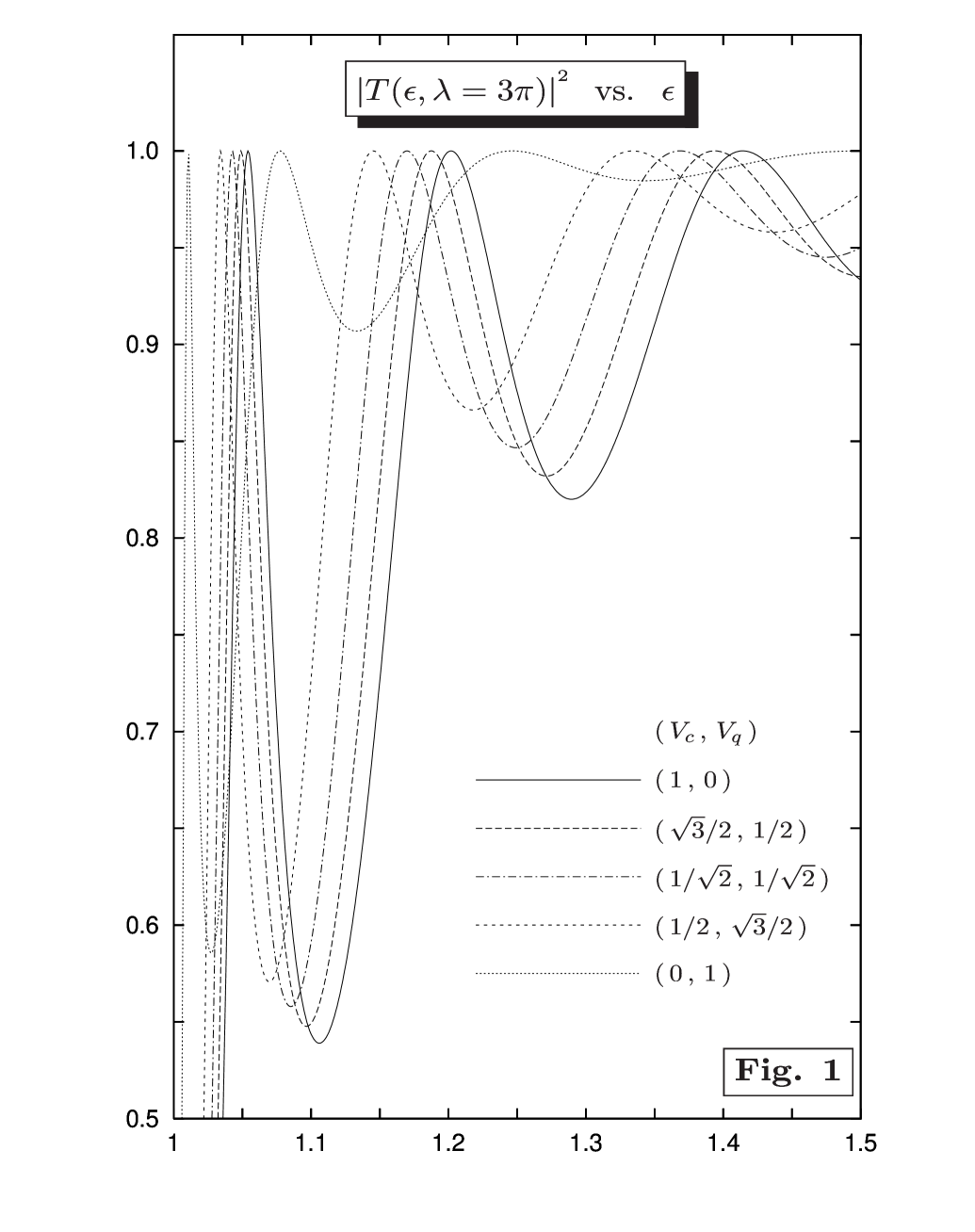
Figure 1: Incoming energy dependence of the transmission probability for different values of the potential. The continuous line represents the standard case of a complex potential. The dotted line represents the case of a pure quaternionic potential. The intermediate cases, show larger values for the minima of the transmission probability when the quaternionic part of the potential increases.

In Fig. 1, where the barrier width is set to $3\pi$, we see the phenomenon of resonance for complex, mixed and pure quaternionic potentials varying the energy of the incoming particle. It is interesting to observe that $\epsilon_{n}$ and $\Delta\epsilon_{n}$ decrease when the quaternionic part of the potential tends to one,

$$\begin{array}[]{|c||c|c|c|c|c|}\hline\cr(\,V_{c}\,,\,V_{q}\,)&\epsilon_{\mbox{\tiny$1$}}&\epsilon_{\mbox{\tiny$2$}}&\Delta\epsilon_{\mbox{\tiny$1$}}&\epsilon_{\mbox{\tiny$3$}}&\Delta\epsilon_{\mbox{\tiny$2$}}\\ \hline\cr\hline\cr(\,1\,,\,0\,)&\,\,1.054&\,\,1.202&\,\,0.148&\,\,1.414&\,\,0.212\\ \hline\cr\hline\cr(\,\sqrt{3}/2\,,\,1/2\,)&1.049&1.188&0.139&1.394&0.206\\ \hline\cr\hline\cr(\,1/\sqrt{2}\,,\,1/\sqrt{2}\,)&1.043&1.170&0.127&1.369&0.199\\ \hline\cr\hline\cr(\,1/2\,,\,\sqrt{3}/2\,)&1.034&1.145&0.111&1.334&0.189\\ \hline\cr\hline\cr(\,0\,,\,1\,)&1.011&1.077&0.066&1.246&0.169\\ \hline\cr\end{array}$$

In Fig. 2, where the incoming energy is set to $\sqrt{2}$, we see the phenomenon of resonance for complex, mixed and pure quaternionic potentials varying the barrier width. It is interesting to observe that $\Delta\lambda$ is constant for a fixed potential and decreases when the quaternionic part of the potential tends to one,

$$\begin{array}[]{|c||c|c|c|c|c|}\hline\cr(\,V_{c}\,,\,V_{q}\,)&\lambda_{\mbox{\tiny$1$}}[\pi]&\lambda_{\mbox{\tiny$2$}}[\pi]&\Delta\lambda_{\mbox{\tiny$1$}}[\pi]&\lambda_{\mbox{\tiny$3$}}[\pi]&\Delta\lambda_{\mbox{\tiny$2$}}[\pi]\\ \hline\cr\hline\cr(\,1\,,\,0\,)&2&3&1&4&1\\ \hline\cr\hline\cr(\,\sqrt{3}/2\,,\,1/2\,)&\,\,1.949&\,\,2.915&\,\,0.966&\,\,3.881&\,\,0.966\\ \hline\cr\hline\cr(\,1/\sqrt{2}\,,\,1/\sqrt{2}\,)&1.890&2.817&0.927&3.744&0.927\\ \hline\cr\hline\cr(\,1/2\,,\,\sqrt{3}/2\,)&1.819&2.695&0.876&3.571&0.876\\ \hline\cr\hline\cr(\,0\,,\,1\,)&1.718&2.478&0.760&3.238&0.760\\ \hline\cr\end{array}$$

IV. THE LIMIT CASE BETWEEN DIFFUSION AND TUNNELING

In this section, we present the interesting case of $\epsilon=1$, i.e. the limit situation between diffusion and tunneling. We start by analyzing this limit for a complex potential $(V_{c},V_{q})=(1,0)$. In the free region, the solution of the Schrödinger equation, for $\epsilon=1$, becomes

$$\Phi_{c,\mbox{\tiny I}}^{\bullet}(\xi) = \exp\left[\,i\,\xi\,\right]+\exp\left[\,-\,i\,\xi\,\right]\,R_{c}^{\bullet}+j\,\exp\left[\,\xi\,\right]\,\widetilde{R}^{\bullet}_{c}\,\,,$$

$$\Phi_{c,\mbox{\tiny III}}^{\bullet}(\xi) = \exp\left[\,i\,\xi\,\right]\,T_{c}^{\bullet}+j\,\exp\left[\,-\,\xi\,\right]\,\widetilde{T}_{c}^{\bullet}\,\,.$$

Eq.(6) reads

$$i\,\partial_{\xi\xi}\,\Phi_{c,\mbox{\tiny II}}^{\bullet}(\xi)=i\,\Phi_{c,\mbox{\tiny II}}^{\bullet}(\xi)-\Phi_{c,\mbox{\tiny II}}^{\bullet}(\xi)\,i\,\,,\,\,\,\,\,\,\,\,\,\,\,\,0<\xi<\lambda\,\,.$$ (20)

Separating the complex from the pure quaternionic part in the solution, i.e.

$$\Phi_{c,\mbox{\tiny II}}^{\bullet}(\xi)=\varphi_{c,\mbox{\tiny II}}^{\bullet}(\xi)+j\,\psi^{\bullet}_{c,\mbox{\tiny II}}(\xi)\,\,,$$

we find two complex differential equations which lead to

$$\varphi_{c,\mbox{\tiny II}}^{\bullet}(\xi) = A_{c}^{\bullet}\,\xi+B_{c}^{\bullet}\,\,,$$

$$\psi^{\bullet}_{c,\mbox{\tiny II}}(\xi) = C_{c}^{\bullet}\,\exp[\,\sqrt{2}\,\xi\,]+D_{c}^{\bullet}\,\exp[\,-\,\sqrt{2}\,\xi\,]\,\,,$$ (21)

observe that only two coefficients appear in the complex solution $\varphi_{c,\mbox{\tiny II}}^{\bullet}(\xi)$. Imposing the continuity conditions, we find

$$R_{c}^{\bullet} = -\,i\,\lambda\,/\,(2-i\,\lambda)\,\,,$$

$$T_{c}^{\bullet} = 2\,\exp[\,-\,i\,\lambda\,]\,/\,(2-i\,\lambda)\,\,,$$ (22)

and as expected $\widetilde{R}_{c}^{\bullet}=\widetilde{T}_{c}^{\bullet}=0$ reproducing the standard complex dynamics. In the case of pure quaternionic potentials, the free solutions are

$$\Phi_{q,\mbox{\tiny I}}^{\bullet}(\xi) = \exp\left[\,i\,\xi\,\right]+\exp\left[\,-\,i\,\xi\,\right]\,R_{q}^{\bullet}+j\,\exp\left[\,\xi\,\right]\,\widetilde{R}^{\bullet}_{q}\,\,,$$

$$\Phi_{q,\mbox{\tiny III}}^{\bullet}(\xi) = \exp\left[\,i\,\xi\,\right]\,T_{q}^{\bullet}+j\,\exp\left[\,-\,\xi\,\right]\,\widetilde{T}_{q}^{\bullet}\,\,,$$

and the equation to be solved is

$$i\,\partial_{\xi\xi}\,\Phi_{q,\mbox{\tiny II}}^{\bullet}(\xi)=j\,e^{-i\theta}\,\Phi_{q,\mbox{\tiny II}}^{\bullet}(\xi)-\Phi_{q,\mbox{\tiny II}}^{\bullet}(\xi)\,i\,\,,\,\,\,\,\,\,\,\,\,\,\,\,0<\xi<\lambda\,\,.$$ (23)

Separating the complex from the pure quaternionic part,

$$\Phi_{q,\mbox{\tiny II}}^{\bullet}(\xi)=\varphi_{q,\mbox{\tiny II}}^{\bullet}(\xi)+j\,\psi^{\bullet}_{q,\mbox{\tiny II}}(\xi)\,\,,$$ (24)

we find, as solutions of the two complex differential equations coming from Eq.(23),

$$\varphi^{\bullet}_{q,\mbox{\tiny II}}(\xi) = A_{q}^{\bullet}\,\xi^{{}^{3}}+B_{q}^{\bullet}\,\xi^{\mbox{\tiny$2$}}+C_{q}^{\bullet}\,\xi+D_{q}^{\bullet}\,\,,$$

$$\psi_{q,\mbox{\tiny II}}(\xi) = -\,i\,e^{-i\theta}\left[\,A_{q}^{\bullet}\,\xi^{{}^{3}}+B_{q}^{\bullet}\,\xi^{\mbox{\tiny$2$}}+(6\,A_{q}^{\bullet}+C_{q}^{\bullet})\,\xi+2\,B_{q}^{\bullet}+D_{q}^{\bullet}\right]\,\,.$$ (25)

By imposing the continuity conditions, we obtain the reflection and transmission amplitudes for pure quaternionic potentials in the limit case between diffusion and tunneling,

$$R_{q}^{\bullet} = -\,i\,\lambda^{{}^{2}}\,(6+4\,\lambda+\lambda^{{}^{2}})\,/\,[\,24+24\,(1-i)\,\lambda-18\,i\,\lambda^{{}^{2}}-4\,(1+i)\,\lambda^{{}^{3}}-\lambda^{{}^{4}}\,]\,\,,$$

$$T_{q}^{\bullet} = 2\,\exp[-i\lambda]\,(12+12\,\lambda+6\,\lambda^{{}^{2}}+\lambda^{{}^{3}})\,/\,[\,24+24\,(1-i)\,\lambda-18\,i\,\lambda^{{}^{2}}-4\,(1+i)\,\lambda^{{}^{3}}-\lambda^{{}^{4}}\,]\,\,.$$ (26)

The expression obtained for $T_{q}^{\bullet}$ is in perfect agreement with the limit for $\epsilon\to 1$ of the coefficient $T$ given in Eq.(13).

The qualitative differences between complex and pure quaternionic potentials can be, for example, seen comparing the reflection and transmission coefficients in the case of thin ($\lambda\ll 1$) and large ($\lambda\gg 1$) barriers. The computation taking into account fourth order corrections gives

$$\begin{array}[]{clcl}\lambda\ll 1\,\,:&|R_{c}^{\bullet}|&\,\,\,\sim&\lambda/2-\lambda^{{}^{3}}/16+\mbox{O}[\,\lambda^{{}^{5}}\,]\,\,,\\ &|T_{c}^{\bullet}|&\,\,\,\sim&1-\lambda^{{}^{2}}/8+3\lambda^{{}^{4}}/128+\mbox{O}[\,\lambda^{{}^{5}}\,]\,\,,\\ \\ &|R_{q}^{\bullet}|&\,\,\,\sim&\lambda^{{}^{2}}/4-\lambda^{{}^{3}}/12+\mbox{O}[\,\lambda^{{}^{5}}\,]\,\,,\\ &|T_{q}^{\bullet}|&\,\,\,\sim&1-\lambda^{{}^{4}}/32+\mbox{O}[\,\lambda^{{}^{5}}\,]\,\,,\\ \\ \lambda\gg 1\,\,:&|R_{c}^{\bullet}|&\,\,\,\sim&1-2/\lambda^{{}^{2}}+6/\lambda^{{}^{4}}+\mbox{O}[\,1/\lambda^{{}^{5}}\,]\,\,,\\ &|T_{c}^{\bullet}|&\,\,\,\sim&2/\lambda-4/\lambda^{{}^{3}}+\mbox{O}[\,1/\lambda^{{}^{5}}\,]\,\,,\\ \\ &|R_{q}^{\bullet}|&\,\,\,\sim&1-2/\lambda^{{}^{2}}-8/\lambda^{{}^{3}}+6/\lambda^{{}^{4}}+\mbox{O}[\,1/\lambda^{{}^{5}}\,]\,\,,\\ &|T_{q}^{\bullet}|&\,\,\,\sim&2/\lambda+4/\lambda^{{}^{2}}-8/\lambda^{{}^{3}}-8/\lambda^{{}^{4}}+\mbox{O}[\,1/\lambda^{{}^{5}}\,]\,\,.\end{array}$$

V. CONCLUSIONS

With the development of a consistent theory of quaternionic differential equations[11, 12, 13, 14, 15, 16], it is now possible to be more profound in discussing quaternionic quantum mechanics. The problem of diffusion by a quaternionic potential, limited up to now to numerical analysis[2, 3, 4, 5, 6, 7, 8, 9, 10], was solved by a matrix approach and leaded to a closed formula for the transmission amplitude.

As in the case of standard quantum mechanics, for incoming particle of energy $\epsilon>1$, quaternionic barriers present the phenomenon of resonances. A comparison between the complex, $V_{c}=1$, and the pure quaternionic, $V_{q}=1$, cases show that, for pure quaternionic potentials, the minimum value of transmission increases whereas the oscillation interval decreases.

This paper could motivate the study of quaternionic quantum mechanics by using the wave packet formalism. An interesting application is the study of tunneling times[21, 22]. The Hartman effect[23] surely represents one of the most intriguing challenges recently appeared in literature[24]. Quaternionic deviations from the standard phase, which is fundamental in the calculation of tunneling times, can be now investigated by using the phase of the transmission coefficient given in this paper.

The analogy between quantum mechanics and the propagation of light through stratified media[25] suggests to analyze in details the limit case $\epsilon=1$. In this case the momentum distributions should be centered in $E_{\mbox{\tiny$0$}}=V_{\mbox{\tiny$0$}}$ and phenomena of diffusion and tunneling must be treated together. The outgoing wave packets should move with different velocity and should give life to new interesting phenomena of interference.

Acknowledgements. One of the authors (SdL) wish to thank the Department of Physics, University of Salento (Lecce, Italy), where the revised version of the paper was prepared, for the invitation and the hospitality. SdL also thanks the FAPESP (Brazil) for financial support by the grant n. 10/02216-2.

Figure 2: Barrier width dependence of the transmission probability for different values of the potential. The continuous line represents the standard case of a complex potential. The dotted line represents the case of a pure quaternionic potential. The intermediate cases, show a shorter oscillation period when the quaternionic part of the potential increases.

References

- [1] S. L. Adler, Quaternionic quantum mechanics and quantum fields (New York, Oxford University Press, 1995).
- [2] A. Peres, “Proposed test for complex versus quaternion quantum theory”, Phys. Rev. Lett. 42, 683–686 (1979).
- [3] H. Kaiser, E. A. George and S. A. Werner, “Neutron interferometric search for quaternions in quantum mechanics”, Phys. Rev. A 29, 2276–2279 (1984).
- [4] A. G. Klein, “Schrödinger inviolate: neutron optical searches for violations of quantum mechanics”, Physica B 151, 44–49 (1988).
- [5] A. J. Davies and B. H. McKellar, “Non-relativistic quaternionic quantum mechanics”, Phys. Rev. A 40, 4209–4214 (1989).
- [6] A. J. Davies and B. H. McKellar, “Observability of quaternionic quantum mechanics”, Phys. Rev. A 46, 3671–3675 (1992).
- [7] S. De Leo, G. Ducati and C. Nishi, “Quaternionic potential in non-relativistic quantum mechanics , J. Phys. A 35, 5411–5426 (2002).
- [8] S. De Leo and G. C. Ducati, “Quaternionic bound states , J. Phys. A 38, 3443–3454 (2005).
- [9] S. De Leo and G. C. Ducati, “Quaternionic diffusion by a potential step , J. Math. Phys. 47, 082106-15 (2006).
- [10] S. De Leo and G. C. Ducati, “Quaternionic wave packets , J. Math. Phys. 48, 052111-10 (2007).
- [11] S. De Leo and G. Scolarici, ”Right eigenvalue equation in quaternionic quantum mechanics”, J. Phys. A 33, 2971–2995 (2000).
- [12] S, De Leo and G. C. Ducati , “Quaternionic differential operators , J. Math. Phys. 42, 2236–2265 (2001).
- [13] S. De Leo, G. Scolarici and L. Solombrino, ”Quaternionic eigenvalue problem”, J. Math. Phys. 43, 5812–2995 (2002).
- [14] S, De Leo and G. C. Ducati , “Solving simple quaternionic differential equations , J. Math. Phys. 44, 2224-2233 (2003).
- [15] S, De Leo and G. C. Ducati , “Real linear quaternionic differential operators , Comp. Math. Appl. 48, 1893-1903 (2004).
- [16] S, De Leo and G. C. Ducati , “Analytic plane wave solution for the quaternionic potential step”, J. Math. Phys. 47, 082106-15 (2006).
- [17] C. Cohen-Tannoudji, B. Diu and F. Lalöe, Quantum mechanics (New York, John Wiley Sons, 1977).
- [18] E. Merzbacher, Quantum mechanics (New York, John Wiley Sons, 1970).
- [19] O. S. Heavens, Optical Properties of Thin Films (Butterworth, London, 1955).
- [20] M. Born and E. Wolf, Principles of optics: electromagnetic theory of propagation, interference and diffraction of light (Oxford, Pergamon Press, 1964).
- [21] E. H. Hauge and J. A. Stovneng, “Tunneling times: a critical review”, Rev. Mod. Phys. 61, 917-936 (1989).
- [22] V. S. Olkhovsky, E. Recami, and J. Jakiel, “Unified time analysis of photon and particle tunneling” , Phys. Rep. 398, 133-178 (2004).
- [23] T. E. Hartman, “Tunneling of a wave packet” , J. Appl. Phys. 33, 3427 (1962).
- [24] H. Winful, “Tunneling time, the Hartman effect, and superluminality: A proposed resolution of an old paradox”, Phys. Rep. 436 1-69 (2006).
- [25] S. De Leo and P. Rotelli, “Localized beams and dielectric barriers”, J. Opt. A 10, 115001-5 (2008).