results from the COMPASS experiment for (GeV/c)2, using high hadrons
Abstract
One of the goals of COMPASS experiment [1] is the determination of the gluon polarisation, , for a deep understanding of the spin structure of the nucleon. The gluon polarisation can be measured via the Photon-Gluon-Fusion (PGF) process. One of the methods to identify this process is selecting high hadron pairs in the final state [2]. The data used for this analysis were collected by the COMPASS experiment during the years 2002 to 2006, using a 160 GeV naturally polarised positive muon beam impinging on a polarised nucleon target. A new result of from high hadron pairs in events with (GeV/c)2 is presented. This result has a better precision due to the addition of 2006 data and an improved analysis based on a neural network approach. The gluon polarisation is also presented in three bins of .
1 The Gluon Polarisation and The High Analysis Formalism
The nucleon spin sum rule can be written in a heuristic way as: , where and are, respectively, the quark and gluon contributions to the nucleon spin and is the orbital angular momentum contribution coming from the partons. The purpose of this analysis is to estimate the gluon polarisation, . The analysis is performed in two complementary kinematic regions: (low ) [3] and (high ) regions. The present work is mainly focused on the analysis for high .
Spin-dependent effects can be measured experimentally using the helicity asymmetry defined as where () and () refer to the parallel and anti-parallel spin helicity configuration of the beam lepton () with respect to the target nucleon ( or ). According to the factorisation theorem in DIS, the (polarised) cross sections can be written as the convolution of the (polarised) parton distribution function, (), the hard scattering partonic cross section, (), and the fragmentation function.
The gluon polarisation is measured directly via the Photon-Gluon Fusion (PGF) process, which allows to probe the spin of the gluon inside the nucleon. To tag this process directly in DIS a high hadron pair data sample is used to calculate the helicity asymmetry. Two other processes compete with the PGF process in leading order QCD approximation, namely the virtual photo-absorption leading order process (LP) and the gluon radiation (QCD Compton) process. The helicity asymmetry for the high hadron pair data sample can thus be schematically written as:
| (1) |
The are the fractions of each process, refers to the different processes. represents the partonic cross section asymmetries, , also known as analysing power. is the depolarisation factor, which is the fraction of the muon beam polarisation transferred to the virtual photon. The virtual photon asymmetry is defined as . This asymmetry is estimated using a parametrisation based on the asymmetry of the inclusive data [4]. A similar equation to (1) can be written to express the inclusive asymmetry of a data sample, .
Using equation (1) for the high hadron pair sample and the above mentioned equation for the inclusive sample the following expression is obtained:
| (2) | ||||||
| (3) | ||||||
| (4) | ||||||
| (5) |
Due to the fact that is present in formula (2) at two different (noted and ), the extraction of requires a definition of the averaged at which the measurement is performed.
2 Data Selection
Data from years 2002 to 2006 are used. These data were obtained from polarised muons of 190 GeV/c scattered off a polarised LiD target at the COMPASS experiment at the CERN SPS. The selected events have an interaction vertex containing an incoming muon and a scattered muon. The data are divided into two sets: the high hadron pair and the inclusive data sample. Both data sets have the kinematic cut applied. Another cut is applied on the fraction of energy taken by the virtual photon, : . These cuts are used to select the inclusive sample.
In the high hadrons data sample, besides the inclusive selection, at least two outgoing high hadrons are required. These so-called hadron candidates must fulfil the following requirements: the hadrons with the highest transverse momentum must have and the hadron with second highest transverse momentum, . This requirement constitutes the high cut.
3 The Weighted Method Approach and The Neural Network for Extraction
The purpose of this analysis is to calculate the gluon polarisation, , in an event-by-event basis using an optimal weight which improves the figure of merit. The asymmetry used for the extraction is related with the experimental helicity asymmetry, , described in section 1, using a weigthing factor . The correct weight, in this case, should take into account all the variables that appear in the set of equations (3) to (5), namely: , where is the dilution factor, the fraction of polarisable target material, is the depolarisation factor, the fraction of muon polarisation is transferred to the virtual photon, is the muon polarisation and is defined in equation 3.
In this analysis it is not possible to tag the events of each involved process, therefore the process fractions and the partonic asymmetries cannot be directly determined from the data samples. To estimate or parametrise these quantities a neural network [5] is used. The neural network is trained by taking as input samples obtained by Monte Carlo (MC) simulation. The result is a parametrisation which is used for the real data to provide the values for all these quantities in an event by event basis.
4 MC Simulation
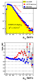
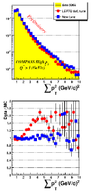
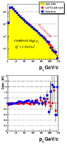
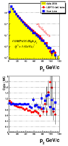
The event simulation is one of the issues of major importance for this analysis since several parameters for the extraction are taken from the simulation. Thus a strong effort was made to achieve a simulation very close to the real data. The MC production comprises three steps: first the events are generated, then the particles pass through a simulated spectrometer using a program based on GEANT 3 [6] and finally the events are reconstructed using the same procedure applied to real data. For the first step the LEPTO 6.5 [7] DIS event generator is used together with a leading order parametrisation of the parton distributions. The fragmentation is based on the Lund string model [8] implemented in JETSET [9]. Figure 1 illustrates the quality of the simulation obtained at the end.
The next step was the tuning of the event generator. The Parton Distribution Function (PDF) set used in this analysis is MSTW2008LO [11]. For the calculation of in LEPTO the ratio is needed. Here the parametrisation of ref. [7] was used. To improve the description of the hadrons, higher order QCD corrections are partially simulated by including gluon radiation in the initial and final states (parton shower – PS) [7]. An extensive and careful tuning of the Lund string fragmentation function parameters and of the hadron intrinsic transverse momentum parameters was performed.
The tuning was done first on the fragmentation function parameters, in this case of the the Lund string function: where ; the parameters are and which are controlled by the JETSET parameters PARJ(41) and PARJ(42).
The second step was the tuning of the hadron intrinsic transverse momentum model, described in [9]. The parameters for this model are PARJ(21), PARJ(23) and PARJ(24), which correspond, respectively, to the sigma of the main Gaussian, to the sigma and to the amplitude fractions for the second Gaussian. The result of all these improvements is the COMPASS tuning.
In figure 1 the kinematic distributions and some hadronic distributions are shown, details can be found in the figures caption. In these figures, two MC simulations with different tunings are shown: the LEPTO default and the COMPASS tuning. In general the COMPASS tuning describes better the data, particularly for the hadronic variables and in which a remarkable agreement between MC and data is presented in the figure. The same applies for the hadron multiplicity (rightmost in figure 1). In table 1 the values of the modified parameters are shown.

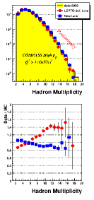
| \brTuning | PARJ(21) | PARJ(23) | PARJ(24) | PARJ(41) | PARJ(42) |
|---|---|---|---|---|---|
| \mrLEPTO Default | 0.36 | 0.01 | 2.0 | 0.3 | 0.58 |
| COMPASS | 0.34 | 0.04 | 2.8 | 0.025 | 0.075 |
| \br |
5 Systematic Studies
The total systematic error is . The contributions come from several sources which were studied in detail. For the neural network, the dependence on the internal structure was taken into account. For the MC several samples with different configurations (tuning, PDF, with and without PS, with and without ) were studied. An extensive study was performed searching for false asymmetries. The dependence of the asymmetry using different parametrisations was studied. For equation (3) two approximations were used for : one with , and another obtained from a second iteration in the neural network of given as input. Also the uncertainty for the input variables related to the polarisation states of the beam and target: , and , were taken into account. The major contributions come from the MC, , and the formula in equation (3), .
6 Results
The gluon polarisation, , is calculated using equations (2) to (5). The result is calculated at . In order to investigate dependence of the data is divided into three bins of the parametrised variable, i.e. divided into three independent samples. These results are given in table 2 and also presented in figure 2. In the same figure, other results from the COMPASS collaboration are also depicted, together with results from HERMES and SMC experiments.
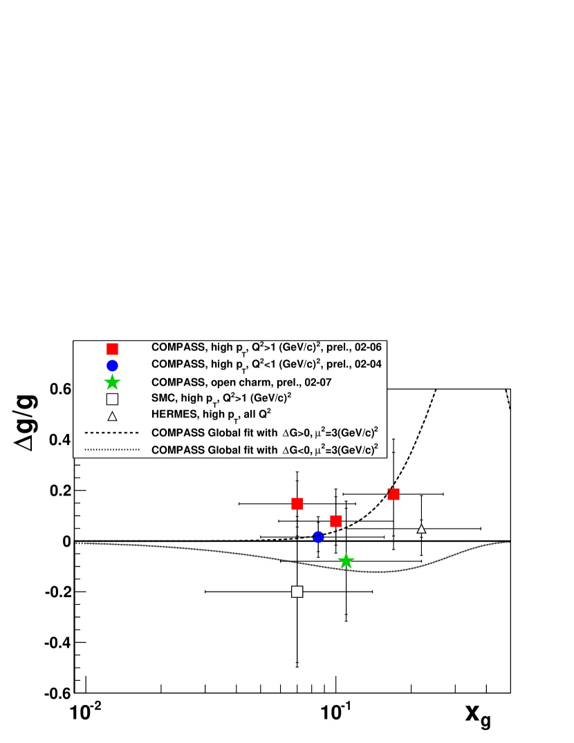
| \br | Bin | Bin | Bin |
|---|---|---|---|
| \mr | |||
| \br |
References
References
- [1] Abbon B, et al.2007 Nucl. Instrum. Meth. A 577 455–518 (Preprint hep-ex/0703049)
- [2] Bravar A, Harrach D and Kotzinian A 1998 Phys. Lett. B 421 349–59 (Preprint hep-ph/9710266)
- [3] Ageev E, et al.2006 Phys. Lett. B 633 25–32 (Preprint hep-ex/0511028)
- [4] Alekseev M, et al.2007 Eur. Phys. J. C 52 255–65 (Preprint hep-ex/0704.1863)
- [5] Sulej R, Zaremba K, Kurek K and Rondio E 2007 Measur. Sci. Tech. 18 2486–90
- [6] Goosssens M 1994 GEANT : Detector Description and Simulation Tool, long writeup W5013 (Geneva: CERN) p 467
- [7] Ingelman G, Edin A and Rathsman J 1997 Comput. Phys. Commun. 101 108–34 (Preprint hep-ph/9605286)
- [8] Andresson B. 1989 The Lund model (Cambridge: Cambridge Univ. Press)
- [9] Sjostrand T 1986 Comput. Phys. Commun. 39 347–407 CPHCB,39,347;
- [10] Botts J, Morfin J, Owens J, Qiu J, Tung W and Weerts H 1993 Phys. Lett. B 304 159–66 (Preprint hep-ph/9303255)
- [11] Martin A, Stirling W, Thorne R and Watt G 2009 Eur. Phys. J. C 63 189–285 (Preprint hep-ph/0901.0002)
- [12] Adeva B, et al.2004 Phys. Rev. D 70 012002
- [13] Airapetian A, et al.2000 Phys. Rev. Lett. 84 2584–8
- [14] Alexakhin V, et al.2007 Phys. Lett. B 647 8–17 (Preprint hep-ex/0609038)