Effective Strategies for Identifying Model Parameters for Open Quantum Systems

Abstract

The problem of identifiability of model parameters for open quantum systems is considered by investigating two-level dephasing systems. We discuss under which conditions full information about the Hamiltonian and dephasing parameters can be obtained. Using simulated experiments several different strategies for extracting model parameters from limited and noisy data are compared.

I Introduction

Control and optimization of quantum systems have been recognized as important issues for many years Blaquiere1 and control theory for quantum systems has been developed since the 1980s Huang2 ; Ong3 ; Clark4 . There has been considerable recent progress in both theory and experiment qcb ; R1-2000 . However, despite this progress, there are still many challenges. Most quantum control schemes rely on open-loop control design based on mathematical models of the system to be controlled. However, accurate models are not often not available, especially for manufactured quantum systems such as artificial quantum dot atoms or molecules. Therefore, system identification 19 is a crucial prerequisite for quantum control.

In the quantum information domain, procedures for characterization of quantum dynamical maps are often known as quantum-process tomography (QPT) 2 ; 3 ; 4 and many schemes have been proposed to identify the unitary (or completely positive) processes, for example, standard quantum-process tomography (SQPT) 1 ; 5 ; 6 , ancilla-assisted process tomography (AAPT) 8 ; 9 ; 10 and direct characterization of quantum dynamics (DCQD) 11 . However, if control of the system’s dynamics is the objective, what we really need to characterize is not a global process but the generators of the dynamical evolution such as the Hamiltonian and dissipation operators. The problem of Hamiltonian tomography (HT), though less well-understood, has also begun to be considered recently by a few authors 15 ; 16 ; 17 ; 18 . Although QPT and HT differ in various regards, both try to infer information about the quantum dynamics from experiments performed on systems, and both can be studied from the point of view of system identification with broad tasks including (1) experimental design and data gathering, (2) choice of model sets and model calculation, and (3) model validation.

Recently the quantum system identification problem has been briefly explored from cybernetical point of view, and underlining the important role of experimental design CDC . In this article we follow this line of inquiry. Throughout the paper, we make the following basic assumptions: (1) the quantum system can be repeatedly initialized in a (limited) set of known states; (2) that we can let the system evolve for a desired time $t$; and (3) that some projective measurements can be performed on the quantum system. The main question we are interested in in this context is how the choice of the initialization and measurement affect the amount of information we can acquire about the dynamics of the system. Given any a limited range of options for the experimental design, e.g., a range of measurements we could perform, different choices for the initial states, or different control Hamiltonians, how to choose the best experimental design, and what are the theoretical limitations? Finally, we are interested in efficient ways to extracting the relevant information from noisy experimental data.

The paper is organized as follows: In Sec. II we discuss the model and basic design assumptions. Sec III deals with the general question of model identifiability in various settings, and in Sec IV we compare several different stategies for parameter estimation from a limited set of noisy data from simulated experiments see how they measure up.

II Model and Design Assumptions

To keep the analysis tractable we consider a simple model of a qubit subject to a Hamiltonian $H$ and a system-bath interaction modelled by a single Lindblad operator $V$, i.e., with system dynamics governed by the master equation

$$\tfrac{\partial\rho(t)}{\partial{t}}=-\tfrac{i}{\hbar}[\hat{H},\rho]+\mathcal{D}[V](\rho),$$ (1)

where the Lindbladian dissipation term is given by

$$\mathcal{D}[V](\rho)=V\rho V^{\dagger}-\tfrac{1}{2}(V^{\dagger}V+VV^{\dagger}).$$ (2)

We shall further simplify the problem by assuming that $V$ is a Hermitian operator representing a depolarizing channel or pure phase relaxation in some basis. Without loss of generality we can choose the basis so that $V$ is diagonal, in fact we can choose $V=\sqrt{\tfrac{\gamma}{2}}\sigma_{z}$ with $\sigma_{z}=\mbox{\rm diag}(1,-1)$ and $\gamma\geq 0$. Under these assumptions the master equation simplifies

$$\mathcal{D}[\sigma_{z}](\rho)=\tfrac{\gamma}{2}(\sigma_{z}\rho\sigma_{z}-\rho).$$ (3)

The control Hamiltonian can be expanded with respect to the Pauli basis $\{\sigma_{x},\sigma_{y},\sigma_{z}\}$

$$H(t)=\tfrac{\hbar}{2}(\omega_{0}(t)\sigma_{z}+\omega_{1}(t)\sigma_{x}-\omega_{2}(t)\sigma_{y})$$ (4)

with possibly time-dependent coefficients $\omega_{\alpha}(t)$. It is convenient to consider a real representation of the system. Following the approach in 20 we expand $\rho$ with respect to the standard Pauli basis for the $2\times 2$ Hermitian matrices

$$\rho=\tfrac{1}{2}(I+v_{x}\sigma_{x}+v_{y}\sigma_{y}+v_{z}\sigma_{z}),$$ (5)

where the coefficients are $v_{\alpha}=\mathop{\rm Tr}(\rho\sigma_{\alpha})$. Similarly expanding the dynamical operators allows us to recast Eq. (1) in following Bloch equation ($\hbar=1$)

$$\begin{pmatrix}\dot{v}_{x}(t)\\ \dot{v}_{y}(t)\\ \dot{v}_{z}(t)\end{pmatrix}=\begin{pmatrix}-\gamma&-\omega_{0}(t)&-\omega_{2}(t)\\ \omega_{0}(t)&-\gamma&-\omega_{1}(t)\\ \omega_{2}(t)&\omega_{1}(t)&0\end{pmatrix}\begin{pmatrix}{v}_{x}(t)\\ {v}_{y}(t)\\ {v}_{z}(t)\end{pmatrix}.$$ (6)

Using this simple model for illustration we subsequently consider the experimental design from three aspects: (1) initialization procedures, (2) measurement choice and (3) Hamiltonian design.

(1) Initialization. We assume the ability to prepare the system in some initial state

$$|\psi_{I}(0)\rangle=\cos\tfrac{\theta_{I}}{2}|0\rangle+\sin\tfrac{\theta_{I}}{2}|1\rangle,$$ (7)

with respect to the basis $\{|0\rangle,|1\rangle\}$, which coincides with the eigenbasis of $V$. We can formally represent the initialization procedure by the operator $\Pi(\theta_{I})$, which is the projector onto the state $|\psi_{I}\rangle$, with $I$ indicating initialization. With these restrictions the design of the initialization procedure is reduced to the selection of parameter $\theta_{I}$. Note that we assume that we can only prepare one fixed initial state, not a full set of basis states.

(2) Measurement. We assume the ability to perform a two-outcome projective measurement

$$M=M_{+}-M_{-}=|m_{+}\rangle\langle m_{+}|-|m_{-}\rangle\langle m_{-}|,$$ (8)

where the measurement basis states can be written as

$$|m_{+}\rangle =\cos\tfrac{\theta_{M}}{2}|0\rangle+\sin\tfrac{\theta_{M}}{2}|1\rangle$$ (9a)

$$|m_{-}\rangle =\sin\tfrac{\theta_{M}}{2}|0\rangle-\cos\tfrac{\theta_{M}}{2}|1\rangle$$ (9b)

so that the choice of the measurement can be reduced to suitable choice of the parameter $\theta_{M}$, and we shall indicate this by writing $M(\theta_{M})$.

(3) Hamiltonian. In practice we may or may not have the freedom to choose the type of Hamiltonian but it will be instructive to consider the identification problem for the following three cases:

• $\omega_{z}(t)\equiv{\omega_{z}}>0$ and $\omega_{x}(t)=\omega_{y}(t)\equiv 0$.

• $\omega_{x}(t)\equiv{\omega_{x}}>0$ and $\omega_{y}(t)=\omega_{z}(t)\equiv 0$.

• $\omega_{y}(t)\equiv{\omega_{y}}>0$ and $\omega_{x}(t)=\omega_{z}(t)\equiv 0$.

In this context the experimental design problem can be reduced to the problem of choosing suitable values $\theta_{I}$ and $\theta_{M}$ to identify the system parameters $\gamma$ and $\omega_{*}$ in each of the three cases above. The problem considered here is similar to that considered in 18 , in particular we still only allow a single initial state and single fixed measurement, but unlike in 18 the initial state and the measurement are not assumed to commute with the dephasing operator.

III Model Identifiability

We now consider the identification problem for the dephasing qubit system, concentrating on experimental design issues for simultaneously discriminating dephasing parameter and Hamiltonian parameter of two-level dephasing systems.

III.1 $H=\omega_{z}\sigma_{z}$, $V=\sqrt{\tfrac{\gamma}{2}}\sigma_{z}$

In this special case $H$ commutes with the dephasing operator $V$. Solving the equation

$$\begin{pmatrix}\dot{v}_{x}(t)\\ \dot{v}_{y}(t)\\ \dot{v}_{z}(t)\end{pmatrix}=\begin{pmatrix}-\gamma&-\omega_{z}&0\\ \omega_{z}&-\gamma&0\\ 0&0&0\end{pmatrix}\begin{pmatrix}{v}_{x}(t)\\ {v}_{y}(t)\\ {v}_{z}(t)\end{pmatrix}$$ (10)

with the initial state (7) gives

$$\begin{pmatrix}{v}_{x}(t)\\ {v}_{y}(t)\\ {v}_{z}(t)\end{pmatrix}=\begin{pmatrix}e^{-\gamma{t}}\cos\omega_{z}t\sin\theta_{I}\\ e^{-\gamma{t}}\sin\omega_{z}t\sin\theta_{I}\\ \cos\theta_{I}\end{pmatrix}$$ (11)

and applying the binary-outcome projective measurement $M(\theta_{M})$ yields the measurement traces $p_{\pm}(t)=\mathop{\rm Tr}[M_{\pm}\rho(t)]$. Defining $\bar{p}_{\pm}(t)=2p_{\pm}(t)-1$, we have

$$\bar{p}_{\pm}(t)=\pm\cos\theta_{I}\cos\theta_{M}{\pm}e^{-\gamma{t}}\cos\omega_{z}t\sin\theta_{I}\sin\theta_{M},$$ (12)

from which we can see that we can obtain information about the system parameters $\omega_{z}$ and $\gamma$ if and only if $\sin\theta_{I}\neq 0$ and $\sin\theta_{M}\neq 0$, i.e., if neither the initial state preparation $\Pi(\theta_{I})$ nor the measurement $M$ commutes with $H$ and $V$. The measurement traces also yield information about $\theta_{I}$ and $\theta_{M}$, i.e., we can determine the relative angles between the initialization and measurement axis and the fixed Hamiltonian/dephasing axis, if they are not known a-priori. We also see that the visibility is maximized if $\sin\theta_{I}\sin\theta_{M}=1$, which will be the case if the initialization and measurement axis are orthogonal to the joint Hamiltonian and dephasing axis.

These results make physical sense. As $[H,V]=0$, if the initial state preparation $\Pi(\theta_{I})$ commutes with $H$ and $V$ then the initial state is a stationary state of the dynamics and the measurement outcome is constant in time $c_{\pm}=\tfrac{1}{2}(1\pm 1)$. If $\sin\theta_{I}\neq 0$ then the initial state is not stationary and the state follows a spiral path towards the joint Hamiltonian and dephasing axis but as both $H$ and $V$ are proportional to $\sigma_{z}$, $\mathop{\rm Tr}[\sigma_{z}\rho(t)]$ is a conserved quantity of the dynamics. If $\sin\theta_{M}=0$ then the measurement commutes with $\sigma_{z}$, and as $\mathop{\rm Tr}[\sigma_{z}\rho(t)]$ is a conserved quantity, we again obtain no information about the dynamics from which to identify the system parameters.

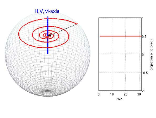
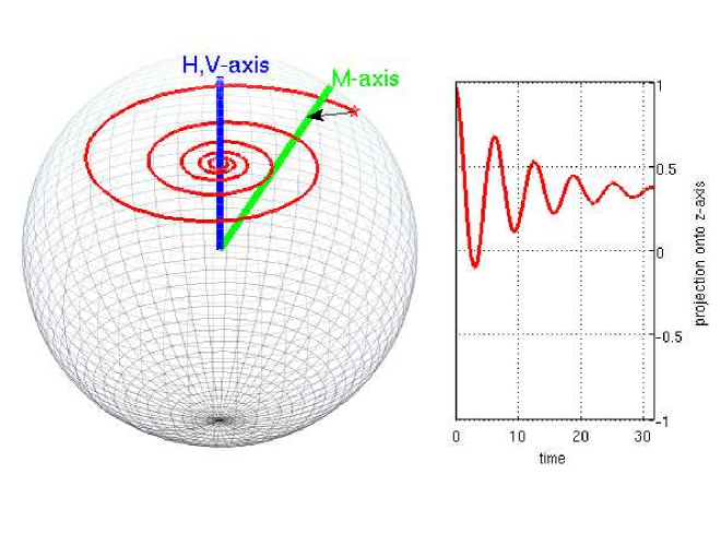
Figure 1: Evolution of system state on the Bloch sphere and projection onto measurement axis for $H=V$: In the pathological case when the measurement axis coincides with the $H,V$-axis, no information about the system parameters can be obtained (left); Otherwise the measurement trace contains information about both $H$ and $V$ (right), provided the initial state is not stationary.

III.2 $H=\omega_{x}\sigma_{x}$, $V=\sqrt{\tfrac{\gamma}{2}}\sigma_{z}$

In this case, the equation (6) is reduced into the following equation

$$\left(\begin{array}[]{c}\dot{v}_{x}(t)\\ \dot{v}_{y}(t)\\ \dot{v}_{z}(t)\end{array}\right)=\left(\begin{array}[]{ccc}-\gamma&0&0\\ 0&-\gamma&-\omega_{x}\\ 0&\omega_{x}&0\end{array}\right)\left(\begin{array}[]{c}{v}_{x}(t)\\ {v}_{y}(t)\\ {v}_{z}(t)\end{array}\right)$$ (13)

and the solution of Eq. (13) for the initial state (7) is

$$\begin{pmatrix}{v}_{x}(t)\\ {v}_{y}(t)\\ {v}_{z}(t)\end{pmatrix}=\begin{pmatrix}e^{-\gamma{t}}\sin\theta_{I}\\ \Phi^{x}_{2}(t)\cos\theta_{I}\\ \Phi^{x}_{3}(t)\cos\theta_{I}\end{pmatrix}$$ (14)

where we set $\widehat{\omega}_{x}=\sqrt{\omega_{x}^{2}-\tfrac{\gamma^{2}}{4}}$ and

$$\Phi^{x}_{2}(t) =-e^{-\tfrac{\gamma}{2}{t}}\tfrac{\omega_{x}}{\widehat{\omega}_{x}}\sin\widehat{\omega}_{x}t$$ (15a)

$$\Phi^{x}_{3}(t) =e^{-\tfrac{\gamma}{2}{t}}[\cos\widehat{\omega}_{x}t+\tfrac{\gamma}{2\widehat{\omega}_{x}}\sin\widehat{\omega}_{x}t].$$ (15b)

If $\omega_{x}^{2}<\gamma^{2}/4$ then $\widehat{\omega}$ will be purely imaginary and the sine and cosine terms above are replaced by the respective hyperbolic functions. If $\omega_{x}^{2}=\gamma^{2}/4$, the expression $\widehat{\omega}^{-1}\sin(\widehat{\omega}t)$ must be analytically continued.

Eq. (14) implies that we can obtain the estimated value of the following probabilities

$$\bar{p}_{\pm}(t)=\pm e^{-\gamma{t}}\sin\theta_{I}\sin\theta_{M}\pm\Phi^{x}_{3}(t)\cos\theta_{I}\cos\theta_{M}.$$ (16)

Noting that $\Phi_{3}^{x}(t)$ depends on both $\omega_{x}$ and $\gamma$ this shows that we can obtain full information about the system parameters if and only if $\cos\theta_{I}\neq 0$ and $\cos\theta_{M}\neq 0$. If $\cos\theta_{I}=0$ or $\cos\theta_{M}=0$ then we can still identify $\gamma$ but not $\omega_{x}$. Again this makes sense.

$\cos\theta_{I}=0$ for $\theta_{I}=\tfrac{\pi}{2}$, i.e., if the initial state is an eigenstate of the Hamiltonian. Since $[H,V]\neq 0$ in this case, eigenstates of $H$ are not stationary. However, since the Hamiltonian and dephasing axis are orthogonal, the initial state remains in a plane orthogonal to the dephasing axis, the $z=0$ plane in our case, following the path $x(t)=e^{-\gamma t}$. Thus we have $[H,\rho(t)]=0$ for all times, and we can therefore not obtain any information about the Hamiltonian parameter $\omega_{x}$, but we can still obtain information about the dephasing parameter $\gamma$. If the Hamiltonian and dephasing axis were not orthogonal then we would expect to be able to identify both the Hamiltonian and dephasing parameters even if the initial state was an eigenstate of $H$ as in this case it would not remain an eigenstate of $H$ under the evolution.

If $\cos\theta_{I}\neq 0$ but $\cos\theta_{M}=0$ then the measurement commutes with the Hamiltonian. Transforming to the Heisenberg picture,

$$\dot{M}_{\pm}(t)=-i[M_{\pm}(t),H]-\tfrac{\gamma}{2}\mathcal{D}[\sigma_{z}]M_{\pm}(t),$$

and again one can show that $M_{\pm}(t)$ remains orthogonal to the dephasing axis and $\mathop{\rm Tr}[M_{\pm}(t)\rho_{0}]=\mathop{\rm Tr}[M_{\pm}\rho(t)]$ is independent of the Hamiltonian $H$, explaining why we cannot obtain any information about $H$ in this case.

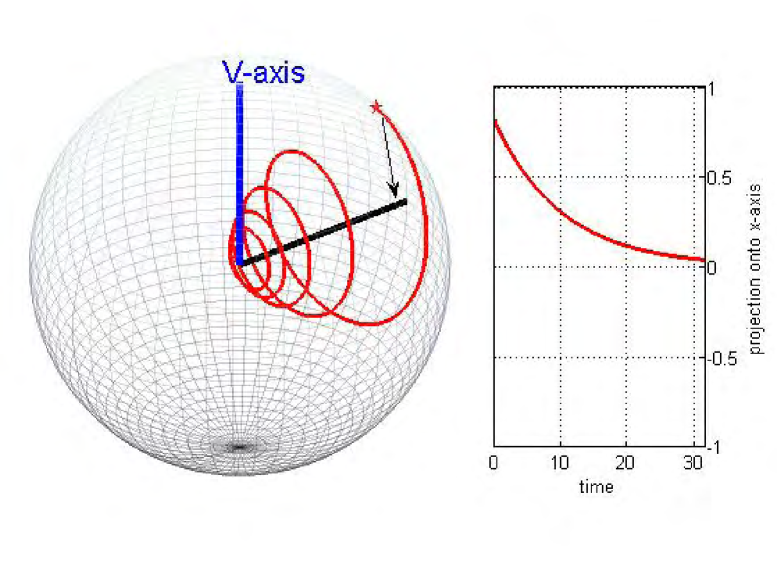
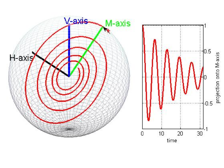
Figure 2: Evolution of system state on the Bloch sphere and projection onto measurement axis for $H\perp V$: If the measurement axis coincides with the $H$-axis, only information about the decoherence parameter $\gamma$ can be obtained (left). In case $C$ the measurement trace always contains information about both $H$ and $V$ (right) for any initial state and measurement.

III.3 $H=\omega_{y}\sigma_{y}$, $V=\sqrt{\tfrac{\gamma}{2}}\sigma_{z}$

In this case equation (6) is reduced into the following equation

$$\begin{pmatrix}\dot{v}_{x}(t)\\ \dot{v}_{y}(t)\\ \dot{v}_{z}(t)\end{pmatrix}=\begin{pmatrix}-\gamma&0&-\omega_{y}\\ 0&-\gamma&0\\ \omega_{y}&0&0\end{pmatrix}\begin{pmatrix}{v}_{x}(t)\\ {v}_{y}(t)\\ {v}_{z}(t)\end{pmatrix}$$ (17)

whose solution for the initial state (7) is

$$\begin{pmatrix}{v}_{x}(t)\\ {v}_{y}(t)\\ {v}_{z}(t)\end{pmatrix}=\begin{pmatrix}\Phi_{23}^{y}(t)\sin\theta_{I}-e^{-\tfrac{\gamma}{2}{t}}\tfrac{\omega_{y}}{\widehat{\omega}_{y}}\sin\widehat{\omega}_{y}t\cos\theta_{I}\\ 0\\ \Phi_{33}^{y}(t)\cos\theta_{I}+e^{-\tfrac{\gamma}{2}{t}}\tfrac{\omega_{y}}{\widehat{\omega}_{y}}\sin\widehat{\omega}_{y}t\sin\theta_{I}\end{pmatrix}$$ (18)

where $\widehat{\omega}_{y}=\sqrt{\omega_{y}^{2}-\tfrac{\gamma^{2}}{4}}$ and

$$\Phi_{23}^{y}(t) =e^{-\tfrac{\gamma}{2}{t}}[\cos\widehat{\omega}_{y}t-\tfrac{\gamma}{2\widehat{\omega}_{y}}\sin\widehat{\omega}_{y}t]$$ (19a)

$$\Phi_{33}^{y}(t) =e^{-\tfrac{\gamma}{2}{t}}[\cos\widehat{\omega}_{y}t+\tfrac{\gamma}{2\widehat{\omega}_{y}}\sin\widehat{\omega}_{y}t]$$ (19b)

This implies that we can obtain the estimated value of the probabilities

$$\bar{p}_{\pm}(t)={\pm}\alpha_{1}e^{-\tfrac{\gamma}{2}{t}}\cos\widehat{\omega}_{y}t\\ \pm\alpha_{2}e^{-\tfrac{\gamma}{2}{t}}\sin\widehat{\omega}_{y}t$$ (20)

where the coefficient functions are

$$\alpha_{1} =\cos(\theta_{I}-\theta_{M})$$ (21a)

$$\alpha_{2} =\tfrac{\gamma}{2\widehat{\omega}_{y}}\cos(\theta_{I}+\theta_{M})+\tfrac{\omega_{y}}{\widehat{\omega}_{y}}\sin(\theta_{I}-\theta_{M}).$$ (21b)

As before, if $\omega_{y}^{2}<\gamma^{2}/4$ then $\widehat{\omega}$ will be purely imaginary and the sine and cosine terms above turn into their respective hyperbolic sine and cosine equivalents, and if $\omega_{y}^{2}=\gamma^{2}/4$, the expression $\widehat{\omega}^{-1}\sin(\widehat{\omega}t)$ must be analytically continued.

In this case it is quite interesting to notice that it is impossible to find such $\theta_{I}$ and $\theta_{M}$ that $\cos(\theta_{I}-\theta_{M})=\sin(\theta_{I}-\theta_{M})=\cos(\theta_{I}+\theta_{M})=0$ and thus that we can identify both model parameters for any choice of the initial state and measurement. This also makes sense because regardless of the choice of $\theta_{I}$ and $\theta_{M}$ the initial state in this case is always orthgonal to the Hamiltonian axis, and the measurement $M$ is always orthogonal to $H$, $[M,H]\neq 0$, there are no conserved quantities and the only stationary state of the system is the completely mixed state.

IV Parameter Estimation

In this section we explore how to estimate dephasing and Hamiltonian parameters from limited noisy measurement data. In an actual experiment we can only estimate the probabilities $p_{\pm}(t)$ at a finite number of times $t_{k}$ by repeatedly initializing the system in some fixed state $\rho_{0}$, and letting it evolve for time $t_{k}$ before performing the projective measurement $M$. Each single repetition of the experiment yields a binary outcome $+1$ or $-1$ and we can estimate the probability $p_{\pm}(t_{k})$ by repeating the experiment $N_{e}$ times and computing the relative frequencies of the respective measurement outcomes $\pm 1$, e.g., $\widehat{p}_{\pm}(t_{k})=\tfrac{N_{\pm}}{N_{e}}$.

To model noisy experimental data we could generate $\widehat{p}_{\pm}(t)$ by adding a zero-mean White-Gaussian noise signal $\widehat{g_{t}}$ to $p_{\pm}(t)$, i.e., $\widehat{p}_{\pm}(t)=p_{\pm}(t)+\widehat{g_{t}}$. By the Law of Large Numbers and Iterated-logarithm Law dong1 this gives a Gaussian distribution $\widehat{p}_{\pm}(t)$ with mean $p_{\pm}(t)$ and variance $\sigma^{2}\sim\tfrac{\log\log N_{e}}{2N_{e}}$ for $N_{e}\rightarrow\infty$. For $N_{e}$ large this should be a good error model, but for small $N_{e}$ it may not accurately capture the nature of the projection noise, which follows a Poisson distribution. To more accurately model noisy experimental data when the number of measurement repetitions is relatively small we can simulate the actual experiment by generating $N_{e}$ random numbers $r_{n}$ between $0$ and $1$, drawn from a uniform distribution, and setting $\widehat{p}_{+}=N_{0}/N_{e}$, where $N_{0}$ is the number of $r_{n}\leq p_{+}$.

IV.1 Fourier and time-series analysis

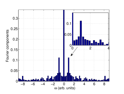
Figure 3: Ideal signal and sparse noisy data points for a simulated experiment assuming Model A with $\omega=1$ and $\gamma=0.1$ (left). We can still identify a peak in the Fourier spectrum (right) around $\omega=1$ but the accuracy of this estimate is limited, and estimating $\gamma$ from the peak broadening would be a challenge.

One commonly used technique to find frequency components in a noisy time-domain signal is the Fourier transform or its discrete version, the discrete or Fast Fourier Transform (FFT). In principle, this allows us to estimate the Hamiltonian parameters (frequencies) $\omega_{z}$, $\hat{\omega}_{x}$ and $\hat{\omega}_{y}$ 17 , and the damping rate $\gamma$ can be estimated from the Lorentzian broadening of the Fourier peak 18 . When the signal is sparse, i.e., we only have a relatively small number of sample points, and noisy, however, this approach becomes problematic. Fig. 3 shows that we can still identify a peak in the spectrum for sparse noisy signals but the accuracy of the estimate is limited, and accurately estimating the dephasing rate $\gamma$ from the broadening of the peak, given the distortion, is very challenging.

Alternatively, once an estimated value for $\omega_{z}$ has been obtained, $\gamma$ can be deduced in other ways. In the simplest case A, where the evolution is given by Eq. (12), we have

$$e^{-\gamma t}\cos\omega_{z}t\sin\theta_{I}\sin\theta_{M}=\bar{p}_{+}(t)-\cos\theta_{I}\cos\theta_{M}$$ (22)

which we can rewrite as

$$\gamma t=-\log\left(\tfrac{\bar{p}_{+}(t)-\cos\theta_{I}\cos\theta_{M}}{\cos\omega_{z}t\sin\theta_{I}\sin\theta_{M}}\right)\buildrel\Delta\over{=}z(t).$$ (23)

Given $\bar{p}_{+}(t)$, if $\theta_{I}$, $\theta_{M}$ and $\omega_{z}$ are known, we can therefore in principle calculate $z(t)$ and thus $\hat{\gamma}$. However, in practice the problem is that $p_{+}(t)$ and all the other parameters are not known precisely. In this case we could estimate $\gamma$ using the Least Square Method zhang1 and the principle of Sequential Analysiszhang2 ; zhang3 .

To explore this approach we generated simulated noisy data signals $\widehat{p}_{+}(t)$ with standard deviation $\sigma_{t}$ according to the procedure above, assuming $\theta_{I}=\theta_{M}=\tfrac{\pi}{2}$, $\omega_{z}=50$, $\gamma=50$ and the sampled period $T_{s}=1.4\mu$s. If the number of measurements $N_{e}$ at each time $t$ is $N_{e}=100$ then the standard deviation of estimated error is $\sqrt{\tfrac{\log\log N_{e}}{2N_{e}}}=0.0874$. The original noiseless probability $\bar{p}_{+}(t)$, the noisy signal with standard deviation $0.0874$ and the power spectral density are shown in Fig.4. Again the frequency $\omega_{z}$ can be easily determined by the peak value in Fig. 4(right). We attempt to determine $\hat{\gamma}$ based on $\widehat{p}_{+}(t)$ using simulated time-series. For a single time series $\widehat{p}_{+}(t)$ the distribution of $\hat{\gamma}$ around the true value of $50$ is shown in Fig. 5(left). The estimation is unsatisfactory even if the signal is sampled densely at a high time resolution. The results can be noticeably improved by averaging over multiple time-series of $\widehat{p}_{+}(t)$. If the mean value of the $\gamma$-estimates over several time series is used as the final estimate for $\gamma$, the estimated error of $\hat{\gamma}$ can be remarkably reduced as shown in Fig. 5 (right), which indicates the mean value of $\hat{\gamma}$ with $1-40$ time-series respectively.

The number of simulated time-series of $\widehat{p}_{+}(t)$ required is determined by the desired estimation accuracy. To achieve a mean value of the distribution of ca. $50$ with standard deviation less than $1.0$ simulations suggest that at least $5$ time-series with $N_{e}=100$ are necessary, i.e., about $500$ measurements have to be performed at each sample time $t$ to ensure that the standard deviation of the estimated error is less than $1.0$. Instead of five time series with $N_{e}=100$ we could choose four times series with $N_{e}=125$ or two with $N_{e}=250$ to reach the nearly same estimation accuracy, as shown in Fig. 6. In the actual experiment one can obtain the mean-value sequence of $\hat{\gamma}$ by continually updating $p(t)$ at each sampled time $t$. If the mean-value sequence is found to converge to a certain fixed value and its standard deviation satisfies the requirement, the experiment measurement should be stopped.

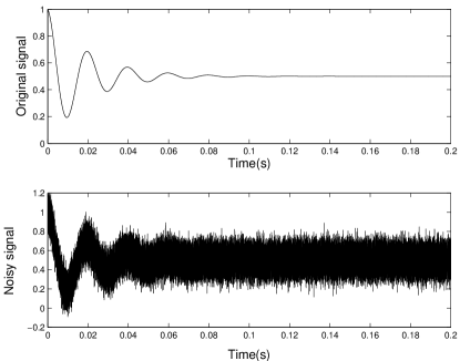
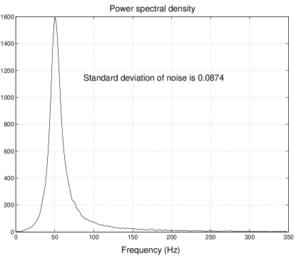
Figure 4: Original time domain signal and simulated noisy signal (left) and power spectral density of noisy signal (right).

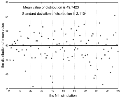
Figure 5: Distribution of $\hat{\gamma}$ based on one simulated time series (left) and mean value of $\hat{\gamma}$ for $1-40$ simulated time series (right).

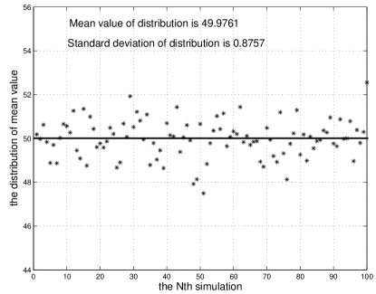
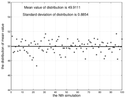
Figure 6: Distribution of mean value of $\hat{\gamma}$ for $N_{e}=125$ using $4$ simulated time series (left), and for $N_{e}=250$ using $2$ simulated time series (right).

To estimate $\gamma$ by finite measurement data one will have to identify a suitable time $t_{d}$ when to terminate the experiment, ideally when the true value of $e^{-\gamma{t_{d}}}$ is almost $0$. A $p_{+}(t)$ is almost equal to $p_{-}(t)$ for $t\geq{t_{d}}$, the signal after this time will be effectively a pure noise signal. Therefore increasing the signal length beyond a certain critical time $t_{k_{0}}$ will not improve the estimation accuracy.

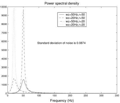
Figure 7: Power spectral density of measured signal in different cases

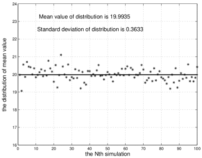
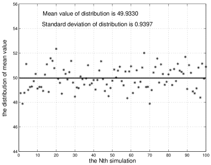
Figure 8: Distribution of mean value of $\hat{\gamma}$ for $\omega_{z}=50Hz$, $\gamma=20$ (left) and $\omega_{z}=20Hz$, $\gamma=50$ (right).

Furthermore, we consider the effect of different $\omega_{z}$ and $\gamma$ on the estimation accuracy. If the true value of $\gamma$ is less than the value of $50$ above, the estimation of $\omega_{z}$ and $\gamma$ will be more accurate (as shown in Fig. 7) as the exponential $e^{-\gamma t}$ decays more slowly. If the value of $\omega_{z}$ is reduced, i.e., the oscillation period is increased while its envelope remains unchanged the accuracy of the estimation is not influenced (as shown in Fig. 8).

IV.2 Bayesian Analysis of Sparse Signals

The previous section shows that we can in principle simultaneously identify both dephasing parameter and Hamiltonian parameters for simple open systems using Fourier and time-series analysis. Both Fourier and time-series analysis can deal with very noisy signals but they require rather dense sampling of the signal with is both time-consuming and resource-intensive. Ideally we would like to be able to estimate the parameters by sparse sampling the signal. One promising approach in this regard is Bayesian estimation. The main idea behind the Bayesian approach is to choose the parameters to be determined, here $\omega$ and $\gamma$, to maximize a certain likelihood function

$$L(\mathbf{p},\mathbf{d},\sigma)=\sigma^{-N}\exp\left[-\frac{||\mathbf{p}-\mathbf{d}||_{2}^{2}}{2\sigma^{2}}\right].$$ (24)

where $\mathbf{d}$ is the measured data and the $\mathbf{p}$ are the probabilities predicted by the model, which depend on the parameters to be determined, and $\sigma$ is the error variance.

Following the same approach as in 16 , we write the signals as a linear combination a small number of basis functions determined by the functional form of the signals. Here the measurement signals $\bar{p}_{\pm}(t)$ can be written as a linear combination of two basis functions

$$\bar{p}_{\pm}(t)=\alpha_{1}g_{1}(t)+\alpha_{2}g_{2}(t).$$ (25)

The values of the basis functions and the coefficients are given in Table 1

	Model A	Model B	Model C
$g_{1}(t)$	$1$	$e^{-\gamma t}$	$e^{-\gamma t/2}\cos(\widehat{\omega}t)$
$g_{2}(t)$	$e^{-\gamma t}\cos(\omega_{z}t)$	$e^{-\gamma t/2}s(t)$	$e^{-\gamma t/2}\sin(\widehat{\omega}t)$
$\alpha_{1}$	$\cos(\theta_{I})\cos(\theta_{M})$	$\sin(\theta_{I})\sin(\theta_{M})$	(21a)
$\alpha_{2}$	$\sin(\theta_{I})\sin(\theta_{M})$	$\cos(\theta_{I})\cos(\theta_{M})$	(21b)

Table 1: Chosen basis functions and coefficients for Bayesian estimation. $s(t)=\cos(\widehat{\omega}t)+\tfrac{\gamma}{2\widehat{\omega}}\sin(\widehat{\omega}t)$. $\widehat{\omega}=\sqrt{\omega^{2}-(\tfrac{\gamma}{2})^{2}}$.

		$\alpha_{1}$			$\alpha_{1}$
	act	est	uncert.	act	est	uncert.
Model A	0.3536	0.3536	0.0133	0.6124	0.5267	0.1393
Model B	0.6124	0.5952	0.0491	0.3536	0.3531	0.0514
Model C	0.9659	1.0066	0.0594	0.2332	0.2506	0.0573

Table 2: Actual and estimated values of the linear coefficients $\alpha_{1}$ and $\alpha_{2}$.

Figs 9–11 show that Bayesian analysis allows us to estimate the model parameters not only for Case A but for all cases, even if the signal is very noisy, the sampling is sparse and the measurement and initialization choices are not ideal to maximize the visibility or signal-to-noise ratio such as $\theta_{M}=\tfrac{\pi}{4}$ and $\theta_{I}=\tfrac{\pi}{3}$. The squeezed peaks indicate that the accuracy of the frequency estimation is much higher than the accuracy of the $\gamma$-estimates.

An additional advantage of the Bayesian estimation does not require a-priori knowledge of the initialization or measurement angles $\theta_{I}$ and $\theta_{M}$. Rather, the estimation procedure provides values for the coefficients of the basis functions, which are related to the parameters $\theta_{I}$ and $\theta_{M}$.

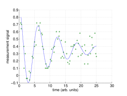
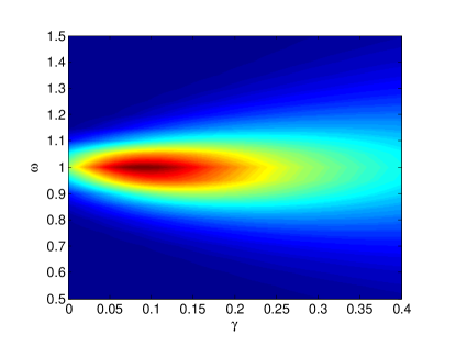
Figure 9: Ideal signal and sparse noisy sampling ($N=75$ samples, signal length $T\approx 25$, accuracy level $N_{e}=100$) (left) and corresponding log-likelihood function (right) for model system A with $\omega_{z}=1$ and $\gamma=0.1$.

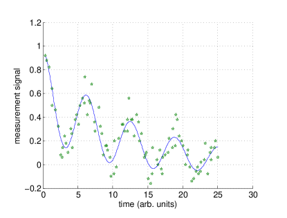
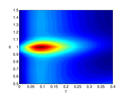
Figure 10: Ideal signal and sparse noisy sampling ($N=100$, $T\approx 25$, $N_{e}=100$) (left) and corresponding log-likelihood function (right) for model system B with $\omega_{x}=1$ and $\gamma=0.1$.

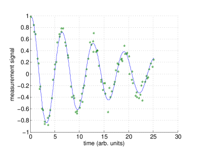
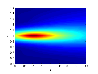
Figure 11: Ideal signal and sparse noisy sampling ($N=100$, $T\approx 25$, $N_{e}=100$) (left) and log-likelihood function (right) for model system C with $\omega_{y}=1$ and $\gamma=0.1$.

V Concluding Discussion

We have studied the issue of model identifiability and experiment design for open system dynamics for a dephasing qubit. From the examples in Sec. III we can derive some general insights about the limits of identifiability and the role of experiment design. Unlike for process tomography, where we require the ability to prepare the system in many different input states, and the ability to measure a complete set of observables, we can in general extract information about both the Hamiltonian and the dephasing parameters by repeating a single experiment, initializing the system in single fixed initial state and measuring a fixed basis. There are certain limitations, however. We gain no information about the value of the system parameters if the initial state is a stationary state of the system, or if the measurement is a conserved quantity, although knowledge of the stationary states or conserved quantities restricts the dynamics and thus provides indirect information about the system. Even if the initial state is not stationary or the measurement is not a conserved quantity, we may fail to obtain information about the Hamiltonian parameters is if the operators $H$ and $V$ are orthogonal and $M$ commutes with $H$, for instance. These limitations also apply to higher dimensional systems, although for such systems additional restrictions on the identifiability of model parameters may arise.

If the experiment design is such that the model parameters are identifiable there are various ways to extract the relevant parameters from a set of noisy samples (time series), including Fourier analysis, time series analysis and Bayesian estimation. Although all of these approaches are in principle able to provide the required information, Bayesian estimation appears to be superior to the alternatives, in particular when we are dealing with a limited number of noisy data points. One reason the Bayesian estimation is capable of providing far more accurate estimates for the parameters given the same input data is that it utilizes information about the structure of the signal in the form of the choice of the basis functions we are projecting onto. This allows us to overcome restrictions on the uncertainties of the parameter estimates imposed by Nyquist’s law.

Appendix A Estimating peak frequency and dephasing rate from Fourier spectrum

Consider a measurement trace of the form

$$a+be^{-\gamma t}\sin(\omega_{0}t),$$ (26)

which corresponds directly to the expected result for Model A if we set $a=\cos(\theta_{I})\cos(\theta_{M})$ and $b=\sin(\theta_{I})\sin(\theta_{M})$. If $\theta_{I}=\theta_{M}=\pi/2$ then $a=0$ and $b=1$. A similar analysis can be done for Models B and C.

The Fourier transform of $u(t)e^{-\gamma t}\sin(\omega_{0}t)$, where $u(t)$ is the Heavyside function, is given by $F(\omega)=\frac{\omega_{0}}{\omega_{0}^{2}+(\gamma+i\omega)^{2}}$. We are interested in its absolute value

$$|F(\omega)|=\frac{\omega_{0}}{[\gamma^{2}+(\omega_{0}-\omega)^{2}][\gamma^{2}+(\omega+\omega_{0})^{2}]}$$ (27)

Differentiating with respect to $\omega$ and setting the numerator to $0$ shows that $|F(\omega)|$ has extrema for $\omega(\omega_{0}^{2}-\gamma^{2}-\omega^{2})=0$, and in particular we have a maximum at $\omega=\sqrt{\omega_{0}^{2}-\gamma^{2}}$ with peak value $(2\gamma)^{-1}$.

Thus, we could in principle estimate both the frequency $\omega_{0}$ and dephasing rate $\gamma$ from the peak height $|F|_{*}$ and position $\omega_{*}$, $\gamma=(2|F|_{*})^{-1}$ and $\omega_{0}=\sqrt{\omega_{*}^{2}+\gamma^{2}}$, but in practice estimating the height of the peak is delicate and this approach is usually very inaccuate.

We can get a better estimate for $\gamma$ using the width of the peak. Let $\omega_{1,2}$ be the (positive) frequencies for which $|F(\omega)|$ assumes half its maximum or $1/(4\gamma)$. Then the full-width-half-maximum $2d$ of $|F(\omega)|$ is $|\omega_{2}-\omega_{1}|$ or

$$d =\left[\sqrt{\omega_{0}^{2}-\gamma^{2}+2\sqrt{3}\omega_{0}\gamma}-\sqrt{\omega_{0}^{2}-\gamma^{2}}\right]$$

$$=\left[\sqrt{\omega_{*}^{2}+2\sqrt{3}\gamma\sqrt{\omega_{*}^{2}+\gamma^{2}}}-\omega_{*}\right]$$

Given the location $\omega_{*}$ and half-width $d$ of the peak we can solve this equation for $\gamma$

$$\gamma=\frac{1}{6}\sqrt{6g(\omega_{*},d)-18\omega_{*}^{2}}$$ (28)

where $g(\omega_{*},d)=\sqrt{9\omega_{*}^{4}+12d^{2}\omega_{*}^{2}+12d^{3}\omega_{*}+3d^{4}}$. Thus, in principle we can determine both the frequency and the dephasing rate by estimating the position and width of the fourier peak.

References

- (1) A. Blaquiere, S. Diner, and G. Lochak, (edit) Information Complexity and Control in Quantum Physics, Springer-Verlag, New York, 1987.
- (2) G. M. Huang, T. J. Tarn, and J. W. Clark, On the Controllability of Quantum Mechanical Systems, J. Math. Phys., vol. 24, pp.2608-2618, 1983.
- (3) C. K. Ong, G. Huang, T. J. Tarn, and J. W. Clark, Invertibility of Quantum Mechanical Control Systems, Math. Sys. Theor., vol.17, pp.335-350, 1984.
- (4) J. W. Clark, C. Ong, T. J. Tarn, and G. M. Huang, Quantum non-Demolition Filters, Math. Sys. Theor., vol.18, pp.33-53, 1985.
- (5) D. D’Alessandro, Introduction to quantum control and dynamics, CRC Press, 2007.
- (6) H. Rabitz, R. de Vivie-Riedle, M. Motzkus and K. Kompa, Whither the Future of Controlling Quantum Phenomena? Science vol.288, 824, 2000.
- (7) L. Ljung, System Identification: Theory for the User, Prentice Hall, Upper Saddle River, New Jersey (2nd Edition) 1999.
- (8) G. M. D’Ariano, M. G. A. Paris, and M. F. Sacchi, Adv. Imaging Electron Phys. 128, 205 (2003).
- (9) G. M. D’Ariano and P. Lo Presti, in Quantum State Estimation, edited by M. Paris and J. Rehacek, Lecture Notes in Physics Vol. 649 Springer, Berlin, 2004 , p. 297.
- (10) L. M. Artiles, R. D. Gill, and M. I. Gu, An invitation to quantum tomography, J. R. Stat. Soc. Ser. B (Stat. Methodol.) vol.67, 109 (2005).
- (11) M. A. Nielsen and I. L. Chuang, Quantum Computation and Quantum Information, Cambridge University Press, Cambridge, UK, (2000)
- (12) I. L. Chuang and M. A. Nielsen, Prescription for experimental determination of the dynamics of a quantum black box, J. Mod. Opt. vol.44, 2455 (1997).
- (13) J. F. Poyatos, J. I. Cirac, and P. Zoller, Complete Characterization of a Quantum Process: The Two-Bit Quantum Gate, Phys. Rev. Lett. vol.78, 390 (1997).
- (14) G. M. D’Ariano and P. Lo Presti, Quantum tomography for measuring experimentally the matrix elements of an arbitrary quantum operation, Phys. Rev. Lett., vol.86, 4195 (2001).
- (15) J. B. Altepeter, D. Branning, E. Jeffrey, T. C. Wei, P. G. Kwiat, R. T. Thew, J. L. O’Brien, M. A. Nielsen, and A. G. White, Ancilla-Assisted Quantum Process Tomography, Phys. Rev. Lett. vol. 90, 193601 (2003).
- (16) G. M. D’Ariano and P. Lo Presti, Imprinting complete information about a quantum channel on its output state, Phys. Rev. Lett. vol. 91, 047902 (2003).
- (17) M. Mohseni and D. A. Lidar, Direct characterization of quantum dynamics, Phys. Rev. Lett. vol.97, 170501 (2006).
- (18) S. G. Schirmer, A. Kolli, and D. K. L. Oi, Experimental Hamiltonian identification for controlled two-level systems, Phys. Rev. A 69, 050306(R) (2004)
- (19) S. G. Schirmer and D. K. L. Oi, Two-Qubit Hamiltonian Tomography by Baysean Analysis of noisy Data, Phys. Rev. A. 80, 022333 (2009); S. G. Schirmer and D. K. L. Oi, Quantum System Identification by Bayesian Analysis of Noisy Data: Beyond Hamiltonian Tomography, Laser Physics 20(5), 1203-1209 (2010)
- (20) Jared H. Cole, Sonia G. Schirmer, Andrew D. Greentree, Cameron J. Wellard, Daniel K. Oi, and Lloyd C. Hollenberg, Identifying an experimental two-state Hamiltonian to arbitrary accuracy, Phys. Rev. A vol.71, 062312 (2005)
- (21) Jared H. Cole, Andrew D. Greentree, Daniel K. L. Oi, Sonia G. Schirmer, Cameron J. Wellard, and Lloyd C. L. Hollenberg Identifying a two-state Hamiltonian in the presence of decoherence, Phys. Rev. A vol.73, 062333 (2006)
- (22) M. Zhang, S. G. Schirmer, H. Y. Dai, W. Zhou and M. Lin. Experimental design and identifiability of model parameters for quantum systems[C] Joint Proceeding of 48th IEEE Conference on Decision and Control and 28th Chinese Control Conference. 2009: 3827-3832.
- (23) R. Alicki and K. Lendi, Quantum Dynamical Semigroups and Applications, Lecture Notes in Physics No. 286 (Springer-Verlag, Berlin, 1987).
- (24) W.Feller, An Introduction to Probability Theory and Its Applications, Vol.1, John Willey & Sons, 3rd edition,1968
- (25) J.O.Berger, Statistical Decision Theory, Springer-Verlag, New York,1980
- (26) A.Wald, Sequential Analysis, John Wiley, New York,1950
- (27) F.J.Anscombe, Sequential Estimation, John Roy. Stat. Soc., Series B,15,1-29,1953