Observational constraints on the modeling of SN 1006

Abstract

Experimental spectra and images of the supernova remnant SN 1006 have been reported for radio, X-ray and TeV gamma-ray bands. Several comparisons between models and observations have been discussed in the literature, showing that the broad-band spectrum from the whole remnant as well as a sharpest radial profile of the X-ray brightness can be both fitted by adopting a model of SN 1006 which strongly depends on the non-linear effects of the accelerated cosmic rays; these models predict post-shock magnetic field (MF) strengths of the order of $150{\,\rm\mu G}$. Here we present a new way to compare models and observations, in order to put constraints on the physical parameters and mechanisms governing the remnant. In particular, we show that a simple model based on the classic MHD and cosmic rays acceleration theories (hereafter the ‘classic’ model) allows us to investigate the spatially distributed characteristics of SN 1006 and to put observational constraints on the kinetics and MF. Our method includes modelling and comparison of the azimuthal and radial profiles of the surface brightness in radio, hard X-rays and TeV $\gamma$-rays as well as the azimuthal variations of the electron maximum energy. In addition, this simple model also provides good fits to the radio-to-gamma-ray spectrum of SN 1006. We find that our best-fit model predicts an effective MF strength inside SN 1006 of $32{\,\rm\mu G}$, in good agreement with the ‘leptonic’ model suggested by the HESS Collaboration (2010). Finally, some difficulties in both the classic and the non-linear models are discussed. A number of evidences about non-uniformity of MF around SN 1006 are noted.

1 Introduction

The supernova remnant (SNR) SN 1006 is one of the most interesting objects for studies of Galactic cosmic rays. It is quite symmetrical with a rather simple bilateral morphology in radio (e.g. Petruk et al., 2009c), nonthermal X-rays (e.g Miceli et al., 2009) and TeV $\gamma$-rays (Acero et al., 2010). Its prominent feature is the positional coincidence of the two bright nonthermal limbs in all these bands, including TeV $\gamma$-rays as demonstrated by recent results of Acero et al. (2010).

Current investigations of SNRs with TeV $\gamma$-ray emission demonstrate an ambiguity in the explanation of the nature of TeV $\gamma$-rays. Namely, the broad-band (radio-to-$\gamma$-rays) spectrum of these SNRs can be fitted by assuming the TeV radiation either as leptonic or as hadronic in origin (e.g. RX J1713.7-3946: Aharonian et al., 2006; Berezhko & Völk, 2006).

The question of the origin of TeV $\gamma$-rays is closely related to the problem of the presence and the role of non-linear effects of cosmic rays acceleration by the forward shock. One of the key parameter distinguishing between these two possibilities is the strength (and thus the nature) of the post-shock magnetic field. The classical picture considers only the compression of the typical interstellar magnetic field (ISMF) $B_{\mathrm{o}}\sim 3{\,\rm\mu G}$ to downstream values of the order of tens $\mu$G. Models including non-linear acceleration (NLA) predict that the ISMF is first amplified upstream due to the back reaction of accelerated protons to $B_{\mathrm{o}}\sim 30{\,\rm\mu}$G and then compressed above hundred $\mu$G. In the former case the inverse-Compton (IC) emission of electrons would be responsible for most of the TeV $\gamma$-rays, in the latter case the proton-origin TeV $\gamma$-ray radiation is expected to be dominant.

The spectrum of SN 1006 may be explained in these two scenarios. One limiting possibility (we call it ‘extreme NLA model’), namely the case of ISMF amplified and compressed to $B_{\mathrm{s}}\approx 150{\,\rm\mu G}$ is considered in details by Berezhko et al. (2009). The model successfully fits the broadband nonthermal spectrum from SN 1006 and the sharpest radial profile of the X-ray brightness. TeV $\gamma$-rays are shown to be produced in both the inverse-Compton mechanism and the pion-decay one, the latter is dominant.

Here, we present a new method to compare models and observations. In particular, we investigate the origin of the patterns of nonthermal images in radio, X-rays and $\gamma$-rays. At present time, this can be done only by using the classic MHD and particle acceleration theories. Therefore, the questions behind the present paper are: may a classical model explain the radio-to-TeV-$\gamma$-ray observations of SN 1006 and can one put observational constraints on some properties of the particle kinetics and/or on the MF?

In this work, we introduce a “classic” model describing SN 1006 and compare the spatial distribution of surface brightness derived from the model with those from observations in different wavelength bands. The comparison will allow us to put some constraints on the parameters of the model, thus deriving some hints on the physical mechanisms governing the cosmic rays acceleration in SN 1006. In the following, the section order is determined by the order of parameters determination: the azimuthal and radial profiles in the radio band are analysed in Sect. 2; the variation of the break frequency in Sect. 3; the broadband spectrum of SN 1006 is calculated in Sect. 4 to check the consistency of our model and to determine the average MF; the X-ray and $\gamma$-ray brightness are investigated in Sect. 5. Finally, we draw our conclusions in Sect. 6.

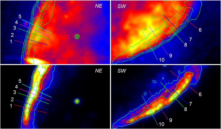
Figure 1: NE and SW limbs of SN 1006 in radio at $\lambda\sim 20{\,\rm cm}$ (top panels) and X-rays with energy 2-4.5 keV (bottom panels) (Petruk et al., 2009c; Miceli et al., 2009). The maximum value of brightness is 100 times the minimum one, in the radio and X-ray images. Radio image is smoothed with Gaussian with $\sigma=0.4^{\prime}$ to lower fluctuations. Color straight lines mark the regions used for extraction of the radial profiles of brightness; length of regions shown is from $0.8R$ to $1.1R$. Green lines represent X-ray contours, linearly spaced.

2 Constraints from radio maps

We consider an SNR expanding through a uniform ISM and uniform ISMF, in the adiabatic stage of its evolution. The Sedov solution is therefore appropriate to describe the hydrodynamics of the system. We consider ideal gas with the adiabatic index $\gamma=5/3$. The MF evolution is treated in the classic framework, without non-linear amplification. Its strength decreases downstream far away from the shoch front and is modelled following Reynolds (1998); the role of the ejecta is considered to be negligible. The classic (unmodified) shock creates the energy spectrum of relativistic electrons in the form $N(E)dE=KE^{-s}\exp(-E/E_{\mathrm{max}})dE$ with the spectral index $s$, normalization $K$ and maximum energy of accelerated electrons $E_{\mathrm{max}}$. Their dependences on obliquity are denoted as $K_{\mathrm{s}}(\Theta_{\mathrm{o}})=K_{\mathrm{s\|}}f_{\mathrm{K}}(\Theta_{\mathrm{o}})$, $E_{\mathrm{max}}(\Theta_{\mathrm{o}})=E_{\mathrm{max\|}}f_{\mathrm{E}}(\Theta_{\mathrm{o}})$ where the symbol ‘$\|$’ marks values at the parallel shock. The downstream evolution of the electron spectrum is modelled as in Reynolds (1998).

2.1 Azimuthal profiles

The symmetrical bright limbs in SN 1006 limit the possible orientations of the ISMF in the plane of the sky. Close to the shock, the azimuthal distribution of the radio surface brightness $S_{\mathrm{r}}$ is mostly determined by $S_{\mathrm{r}}(\varphi)\propto\varsigma(\varphi)\ \sigma_{\mathrm{B}}(\varphi)^{(s+1)/2}$ (Petruk et al., 2009c) where $\varsigma$ is the injection efficiency (a fraction of accelerated electrons), $\sigma_{\mathrm{B}}$ the compression factor for MF (unity for parallel and 4 for perpendicular shock), $\varphi$ the azimuthal angle. If the injection is isotropic, $\varsigma(\Theta_{\mathrm{o}})=\mathrm{const}$ where $\Theta_{\mathrm{o}}$ is the obliquity angle), then the bright radio limbs correspond to projection of the equatorial belt with NW-SE orientation of the ISMF (BarMF or barrel-like model). If, on the other hand, the injection prefers quasi-parallel shocks, the bright limbs of SN 1006 are two polar caps and the ISMF should be oriented in the NE-SW direction (CapMF model).

The ISMF creates an aspect angle $\phi_{\mathrm{o}}$ with the line of sight. Recently, Petruk et al. (2009c) have shown that the comparison of the experimental azimuthal profiles of the radio brightness with those derived from theoretically synthesized radio images can be a powerful tool to determinethe model of electron injection, the MF orientation in the plane of the sky and the aspect angle $\phi_{\mathrm{o}}$. In particular, these authors have shown that, under the assumptions of uniform ISMF/ISM, the injection is be isotropic, the 3D morphology of the remnant is BarMF and the aspect angle is $\phi_{\mathrm{o}}=70^{\mathrm{o}}$ (these results were confirmed recently by detailed MHD calculations of Schneiter et al., 2010). For the sake of generality, we explore in the next subsection also the CapMF model with the same value of $\phi_{\mathrm{o}}$.

2.2 Radial profiles

The post-shock value (denoted hereafter by the index ‘s’) of the spectrum normalization $K_{\mathrm{s}}$ is proportional to the injection efficiency $\varsigma$. The injection efficiency may vary with the shock strength (velocity). We assume that $K_{\mathrm{s}}\propto V^{-b}$ where $V$ is the shock velocity, and $b$ is a parameter.

In Appendix A.1, we show that the surface brightness distribution of a Sedov SNR in the radio band is

$$S_{\mathrm{r}}=\mathrm{const}\ {\cal S}_{\mathrm{r}}(\bar{\rho},\varphi;\phi_{\mathrm{o}},b)\ \nu^{-(s-1)/2}K_{\mathrm{s\|}}B_{\mathrm{o}}^{(s+1)/2}R$$ (1)

where $\bar{\rho}=\rho/R$, and $\rho$ is the coordinate along the radius of the remnant $R$. ${\cal S}_{\mathrm{r}}$ accounts for the evolution of the electron energy spectrum and MF inside the SNR. For fixed $\varphi$, ${\cal S}_{\mathrm{r}}(\bar{\rho})$ is an universal profile which, for a given dependence of $\varsigma(\Theta_{\mathrm{o}})$, aspect angle $\phi_{\mathrm{o}}$ and index $s$, depends only on the parameter $b$.

We use the experimental radio image of SN 1006 presented in Petruk et al. (2009c) to determine the parameter $b$. We extract the radial profiles of radio brightness from the regions shown in Fig. 1. The profiles are reported in Fig. 2 together with the theoretical profiles ${\cal S}_{\mathrm{r}}(\bar{\rho};b)$ calculated numerically for three values of $b=-1,0,1$. Close to the shock front, the experimental profiles seems to be between the theoretical ones calculated for $b=-1$ and $b=0$.

On the other hand, Fig. 2 shows also that the theoretical profiles of radio brightness calculated from a Sedov model of SNR expanding through a uniform ISM/ISMF do not fit the experimental data to larger extent, namely for $\rho<0.94R$ (see the inset in Fig. 2). This result may be explained if either the ISMF or the ISM in the neighbourhood of SN 1006 is not uniform. In fact, the radio brightness is higher where either the ISMF strength $B_{\mathrm{o}}$ or the ISM density $n_{\mathrm{o}}$ is larger: $S_{\mathrm{r}}\propto\varsigma\sigma_{\mathrm{B}}^{(s+1)/2}\propto n_{\mathrm{o}}B_{\mathrm{o}}^{(s+1)/2}$. As a consequence, a gradient of ISMF/ISM can cause various asymetries in the brightness distribution of the remnant (Orlando et al., 2007); e.g. if the gradient has a component along the line of sight, it may increase the brightness inside the projection depending on its orientation and strength (Petruk, 2001). The radio profiles from the SW limb support such a scenario: they monotonically increase from the shock to $\simeq 0.85R$ (Fig. 1) while the maximum of the radio brightness in Sedov SNR should be located around $\simeq 0.97R$. We investigate the effects of a nonuniform ISMF on the remnant morphology in a companion paper (Bocchino et al. 2010, in preparation), where we consider an MHD model of SNR expanding through a nonuniform ISMF and compare the synthetic images in the radio band with observations of SN 1006. In the present study, we adopt $b=0$.

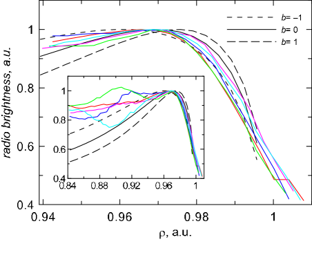
Figure 2: Radial profiles of the radio brightness in NE limb of SN 1006. Experimental profiles (from regions 1-5, Fig. 1) are in color. Theoretical profiles are in black, for $b=-1$ (dot), $b=0$ (solid), $b=1$ (dashed). They are calculated for $s=2$, $\phi_{\mathrm{o}}=70^{\mathrm{o}}$, isotropic injection and $\varphi=70^{\mathrm{o}}$ (observational profiles are taken for $\varphi=65^{\mathrm{o}}-75^{\mathrm{o}}$). Internal plot is a zoom-out of the main figure.

3 Constraints from obliquity dependence of the maximum energy

In this section, we aim at deriving some constraints on the modeling of SN 1006 from the obliquity dependence of the maximum energy deduced from the observations. Miceli et al. (2009) considered a set of 30 regions covering the entire rim of the shell of SN 1006. The spectral fitting of the X-ray emission extracted from these regions allowed to derive the azimuthal variation of $\nu_{\mathrm{break}}$, a parameter in the srcut model of XSPEC which is related to the maximum energy of electrons as

$$E_{\mathrm{max}}=c_{1}^{-1/2}\nu_{\mathrm{break}}^{1/2}B_{\mathrm{s}}^{-1/2}$$ (2)

where $B_{\mathrm{s}}$ is the strength of the post-shock MF, $c_{1}=6.26\times 10^{18}{\,\rm cgs}$. We use the above relation together with the experimental data on $\nu_{\mathrm{break}}$ to determine the azimuthal variation of the electron maximum energy $E_{\mathrm{max}}(\varphi)$.

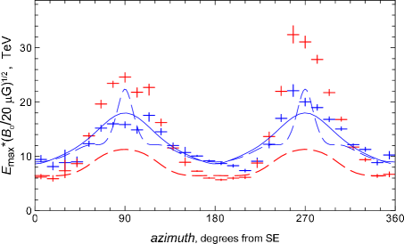
Figure 3: Variation of $E_{\mathrm{max}}$ (shown with vertical one-sigma errors) over the forward shock in SN 1006, obtained from experimental data on $\nu_{\mathrm{break}}$ (Miceli et al., 2009) and Eq. (2), for two models of ISMF: BarMF (blue crosses), CapMF (red crosses). Aspect angle $\phi_{\mathrm{o}}=70^{\mathrm{o}}$. Dashed red line: the loss-limited model with $\eta=1$, CapMF. Solid blue line: the time-limited model with $\eta=1.5$, BarMF. Dashed blue line: the loss-limited model with $\eta=7.6$, BarMF.

The dependence of $E_{\mathrm{max}}$ on the obliquity angle $\Theta_{\mathrm{o}}$ can be represented as $E_{\mathrm{max}}(\Theta_{\mathrm{o}})=E_{\mathrm{max\|}}f_{\mathrm{E}}(\Theta_{\mathrm{o}})$ where $f_{\mathrm{E}}(\Theta_{\mathrm{o}})$ is a smooth function of $\Theta_{\mathrm{o}}$. The azimuthal profiles of $E_{\mathrm{max}}$ determined with Eq. (2) for two different configurations of the ISMF (BarMF and CapMF) is shown on Fig. 3.

What cause the limitation of $E_{\mathrm{max}}$ in SN 1006? In the framework of the classical theory of acceleration, Reynolds (1998) (to which the reader is referred to for more details) developed three different theoretical models for the surface variation of $E_{\mathrm{max}}$ (and, therefore, for its obliquity dependence). Namely, the maximum energy of accelerated electrons may be determined: 1) by the electron radiative losses (in the following loss-limited model), 2) by the limited time of acceleration (time-limited model), and 3) by escaping of particles from the region of acceleration (escape-limited model). The third model results in constant $E_{\mathrm{max}}$ that contradicts the obliquity dependence of $E_{\mathrm{max}}$ derived from observations (Miceli et al. 2009; see Fig. 3). Therefore, we do not consider it in the rest of the paper. In the other two models, $f_{\mathrm{E}}(\Theta_{\mathrm{o}})$ depends basically on the MF compression ratio $\sigma_{\mathrm{B}}$, and on the level of turbulence which is reflected by the “gyrofactor” $\eta\geq 1$, i.e. the ratio between the mean free path of particle along the magnetic field and its Larmour radius (see Reynolds 1998). Figure 4 shows the obliquity dependence of $E_{\mathrm{max}}$ in the time-limited and loss-limited models for different $\eta$.

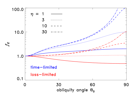
Figure 4: Obliquity dependence of the function $f_{\mathrm{E}}(\Theta_{\mathrm{o}})$, determining the azimuthal dependence of $E_{\mathrm{max}}$. The blue solid line and red solid line correspond to the time-limited and loss-limited model of Reynolds (1998). Dotted and dashed lines correspond to the same models but using different values for the gyrofactor $\eta$.

The obliquity angle is minimum in SN 1006 at azimuth $0^{\mathrm{o}}$ for BarMF and at azimuth $90^{\mathrm{o}}$ for CapMF. Therefore, $E_{\mathrm{max}}$ is expected to increase or decrease with obliquity for BarMF and CapMF respectively (Fig. 3). In the loss-limited model of $E_{\mathrm{max}}$, the function $f_{\mathrm{E}}(\Theta_{\mathrm{o}})$ increases with increasing obliquity for $\eta\geq 3$ (red lines in Fig. 4). In the time-limited model, the function $f_{\mathrm{E}}(\Theta_{\mathrm{o}})$ increases with obliquity for any $\eta$ (blue lines in Fig. 4). In contrast, Fig. 3 shows decrease of $E_{\mathrm{max}}$ from $\varphi=90^{\mathrm{o}}$ to $180^{\mathrm{o}}$ for CapMF (red crosses). Thus, the time-limited model and loss-limited model with $\eta\geq 3$ are not applicable if one considers a polar-caps morphology of SN 1006. In the loss-limited case, the fastest decrease with obliquity is for $\eta=1$ but it does not fit the experimental profile of $E_{\mathrm{max}}$ for model CapMF (red dashed line on Fig. 3). To the end, the NE-SW orientation of ISMF (CapMF, polar caps) is not able to explain observed azimuthal variation of $\nu_{\mathrm{break}}$, under assumptions of uniform ISMF/ISM and classic MHD/acceleration. We tried also other aspect angles, $\phi_{\mathrm{o}}>50^{\mathrm{o}}$, either with or without the inclusion of IC radiative losses. However, the conclusion remains unchanged.

In the BarMF case (blue crosses), the function $f_{\mathrm{E}}(\Theta_{\mathrm{o}})$ for SN 1006 may be determined by fitting the experimental data with a model of Reynolds (1998). The best-fit in the time-limited model is reached for $\eta=1.5\pm 0.02$ ($\chi^{2}/\mathrm{dof}=12.7$, solid blue line on Fig. 3). The best-fit for the loss-limited model is for $\eta=7.6\pm 0.11$ ($\chi^{2}/\mathrm{dof}=25.8$, dashed blue line) but the shape of the fit does not follow well the observed one.

Thus, the azimuthal variation of $\nu_{\mathrm{break}}$ may be explained in the framework of the classic MHD/acceleration theories. It limits ISMF orientation to only BarMF configuration, in agreement with the same conclusion obtained from azimuthal fits of the radio surface brightness (Petruk et al., 2009c). The time-limited model of Reynolds (1998) with $\eta=1.5$ is the most appropriate for $E_{\mathrm{max}}(\Theta_{\mathrm{o}})$; we use it in the present paper. In this model, the maximum energy of accelerated electrons varies with time very slowly (Reynolds, 1998). We assume therefore that $E_{\mathrm{max}}$ is independent on the shock velocity. Similar conclusions are obtained by Katsuda et al. (2010): the correlation they found between the X-ray flux and the cut-off frequency is against the loss-limited model for $E_{\mathrm{max}}$; absence of time variation of the synchrotron flux supports assumption about constant (in time) maximum energy.

The solid blue line in Fig. 3 shows that $E_{\mathrm{\max}}=8.5(B_{\mathrm{o}}/20{\,\rm\mu G})^{-1/2}{\,\rm TeV}$ at azimuth $\varphi=0$. Since the aspect angle $\phi_{\mathrm{o}}=70^{\mathrm{o}}$, this value of $E_{\mathrm{\max}}$ corresponds therefore to the obliquity $\Theta_{\mathrm{o}}=20^{\mathrm{o}}$. It is smaller at the parallel shock, namely $E_{\mathrm{\max\|}}=0.644E_{\mathrm{\max}}$ for $\eta=1.5$ (Reynolds, 1998). Therefore,

$$E_{\mathrm{\max\|}}=5.4\left(\frac{B_{\mathrm{o}}}{20{\,\rm\mu G}}\right)^{-1/2}{\,\rm TeV}.$$ (3)

The same time-limited model predicts $E_{\mathrm{\max\bot}}=3.25E_{\mathrm{\max\|}}$.

4 Constraints from total radio, X-ray and TeV gamma-ray spectrum

In the calculations of the synchrotron spectrum, the self-similarity of Sedov solutions allows us to represent the complex picture of the synchrotron emission from the whole SNR (which includes the complicate description of the downstream evolution of the fluid elements, the magnetic field and the spectrum of relativistic electrons in the SNR interior as well as the full single-electron emissivity convolved at each point with the electron spectrum) by a single universal constant $\zeta$ and a modification factor $\eta_{\mathrm{syn}}$. The former is a (reduced) integral of the radio emissivity over the SNR volume; the latter reflects the deviation of the X-ray spectrum from the power-law (for more details see Appendix B.1). $\eta_{\mathrm{syn}}$ is defined as a ratio of the integral (i.e. from the whole SNR) synchrotron flux at a given frequency (e.g. at the X-rays) to the power-law extrapolation of the radio flux to this frequency; obviously, $\eta_{\mathrm{syn}}\leq 1$.

In a broad band (from radio to X-rays), the synchrotron spectrum of the volume-integrated emission from the whole SNR may be represented by (Appendix B.1)

$$F_{\mathrm{syn}}({\nu})=C_{\mathrm{r}}\zeta{\nu}^{-(s-1)/2}\eta_{\mathrm{syn}}(\tilde{\varepsilon};\epsilon_{\mathrm{f\|}})B_{\mathrm{o}}^{(s+1)/2}K_{\mathrm{s\|}}R^{3}d^{-2}$$ (4)

where $C_{\mathrm{r}}$ is a constant, and $d$ the distance to SNR. The constant $\zeta$ is different for different models (Appendix B.1); it is $\zeta=2.68$ for $s=2.0$ or $\zeta=2.77$ for $s=2.1$ in our reference model of SN 1006 (namely BarMF, with isotropic injection and $b=0$).

The reduced photon energy is defined as $\tilde{\varepsilon}=\tilde{\nu}=\nu/\nu_{\mathrm{c}}(E_{\mathrm{max\|}},B_{\mathrm{o}})$, $\nu_{\mathrm{c}}(E,B)=c_{1}\left\langle\sin\phi\right\rangle E^{2}B$ is the synchrotron characteristic frequency:

$$\tilde{\varepsilon}=9.5\ \varepsilon_{\mathrm{keV}}\left(\frac{E_{\mathrm{max\|}}}{10{\,\rm TeV}}\right)^{-2}\left(\frac{B_{\mathrm{o}}}{20{\,\rm\mu G}}\right)^{-1},$$ (5)

where $\varepsilon_{\mathrm{keV}}$ is the photon energy in keV. With Eq. (3), this becomes $\tilde{\varepsilon}=32.6\varepsilon_{\mathrm{keV}}$.

The reduced fiducial energy $\epsilon_{\mathrm{f}}=637\left(B_{\mathrm{s}}^{2}tE_{\mathrm{max}}\right)^{-1}$ is one of the key parameter for modeling the X-ray and $\gamma$-ray emission (Reynolds, 1998). The energy $\epsilon_{\mathrm{f}}$ is a measure of the importance of radiative losses in modification of the high-energy end of the electron spectrum and therefore of the X-ray and $\gamma$-ray spectra and images: radiative losses are essential for $\epsilon_{\mathrm{f}}<1$; if $\epsilon_{\mathrm{f}}>1$, the adiabatic losses are dominant even for electrons with $E\sim E_{\mathrm{max}}$ (Reynolds, 1998). With Eq. (3) and the age $t=1000{\,\rm yrs}$, the dimensionless fiducial energy at parallel shock is

$$\epsilon_{\mathrm{f\|}}=5.8\left(\frac{B_{\mathrm{s\|}}}{20{\,\rm\mu G}}\right)^{-3/2},$$ (6)

where $\epsilon_{\mathrm{f\bot}}$ is $\sigma_{\mathrm{B}}^{2}E_{\mathrm{\max\bot}}/E_{\mathrm{\max\|}}=52$ times smaller because both $B_{\mathrm{s}}$ and $E_{\mathrm{\max}}$ are larger at the perpendicular shock.

The modification factor $\eta_{\mathrm{syn}}({\nu})$ shows how the synchrotron spectrum $F_{\mathrm{syn}}({\nu})$ deviates from the power-law dependence ${\nu}^{-(s-1)/2}$. The modification factor is defined to be $\eta_{\mathrm{syn}}=1$ for the radio band; it is effective in the X-ray band and rather quickly approaches to unity with $\nu$ decreasing below $\nu_{\mathrm{c}}(E_{\mathrm{max}},B)$.

In a similar fashion, the spectral distribution of the IC emission from the whole SNR is (Appendix B.2)

$$F_{\mathrm{ic}}(\nu)=C_{\mathrm{T}}\zeta_{\mathrm{T}}\nu^{-(s-1)/2}\eta_{\mathrm{ic}}(\nu,\epsilon_{\mathrm{f\|}},E_{\mathrm{max\|}})K_{\mathrm{s\|}}R^{3}d^{-2}.$$ (7)

where $\eta_{\mathrm{ic}}$ is the modification factor and $\zeta_{\mathrm{T}}$ the universal constant for IC $\gamma$-rays (exact definitions are given in Appendix B.2). For our reference model of SN 1006 (BarMF, with isotropic injection, and $b=0$), $\zeta_{\mathrm{T}}=0.81$ for $s=2$ and $\zeta_{\mathrm{T}}=0.79$ for $s=2.1$.

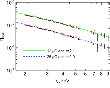
Figure 5: The modification factors $\eta_{\mathrm{syn}}$ in X-rays calculated from our reference model for two sets of parameters, namely $B_{\mathrm{o}}=25{\,\rm\mu G}$ and $s=2.0$ (dashed blue line), and $B_{\mathrm{o}}=12{\,\rm\mu G}$ and $s=2.1$ (solid green line). The corresponding modification factors derived from the SUZAKU data (Bamba et al., 2008, black and red crosses represent XIS spectra from the front-illuminated CCDs and back-illuminated CCD respectively) are also shown for the cases $s=2.0$ (lower) and $s=2.1$ (upper).

4.1 Fit to the radio spectrum

Miceli et al. (2009) measured the radio-to-X-ray photon index $\alpha=(s-1)/2$ of the non-thermal component for each of the 30 regions selected to cover the entire rim of the shell of SN 1006, finding $\alpha\approx 0.5$. This value is almost within 1-$\sigma$ error of the best-fit value $\alpha=0.6_{-0.09}^{+0.08}$ (Allen et al., 2008), obtained for the radio fluxes from SN 1006 at 8 different radio frequencies (most of the fluxes are from Milne, 1971). We consider therefore $\alpha=0.5$ as possible choice for the spectral index of the synchrotron spectrum. The best-fit ($\chi^{2}/\mathrm{dof}=1.0$) for these radio data and fixed $\alpha=0.5$ is

$$F_{\mathrm{r,obs}}(\nu)=18.4\left({\nu}/{1\mathrm{\ \!GHz}}\right)^{-0.5}{\,\rm Jy}.$$ (8)

In addition, we consider also the case $\alpha=0.55$ (i.e. $s=2.1$), a value successfully used in the broad-band model of the synchrotron and IC spectrum of SN 1006 (Acero et al., 2010). The best-fit ($\chi^{2}/\mathrm{dof}=0.56$) for the same radio data and fixed $\alpha=0.55$ is

$$F_{\mathrm{r,obs}}(\nu)=18.1\left({\nu}/{1\mathrm{\ \!GHz}}\right)^{-0.55}{\,\rm Jy}.$$ (9)

4.2 Fit to the X-ray spectrum

Figure 5 compares the X-ray modification factor derived from our reference model with that derived from observations for two different sets of parameters ($B_{\mathrm{o}}$, $s$). Note that the use of the modification factor allows us to avoid uncertainties in the distance of the remnant, its radius, and the density of emitting electrons. The experimental modification factor $\eta_{\mathrm{syn,obs}}$ is calculated from the SUZAKU X-ray spectrum $F_{\mathrm{x,obs}}$ of the whole remnant SN 1006 (Fig. 6 in Bamba et al., 2008) as the ratio of the observed X-ray spectrum to the extrapolation of the radio spectrum to X-rays

$$\eta_{\mathrm{syn,obs}}(\nu)={F_{\mathrm{x,obs}}(\nu)\over F_{\mathrm{r,obs}}(\nu)}.$$ (10)

This definition together with Eqs. (5) and (3) make the modification factor $\eta_{\mathrm{syn,obs}}(\tilde{\nu})$ essentially independent on the MF. Theoretical $\eta_{\mathrm{syn}}(\tilde{\varepsilon};\epsilon_{\mathrm{f\|}})$, for fixed values of $s$, $b$, $f_{\mathrm{K}}(\Theta_{\mathrm{o}})$ and $f_{\mathrm{E}}(\Theta_{\mathrm{o}})$ is a function of the reduced fiducial energy $\epsilon_{\mathrm{f\|}}$ only. This parameter reflects the efficiency of the radiative losses on the evolution of electrons with energies around $E_{\mathrm{max}}$ and, therefore, on the shape of the synchrotron X-ray spectrum. In SN 1006, it is related to $B_{\mathrm{o}}$ through Eq. (6).

The strength of the ambient MF $B_{\mathrm{o}}=25{\,\rm\mu G}$ together with $s=2.0$ provide agreement between the X-ray modification factors derived from our reference model and from the observations (Fig. 5 blue line). A smaller value of the MF strength, $B_{\mathrm{o}}=12{\,\rm\mu G}$, fits the SUZAKU spectrum if $s=2.1$ (Fig. 5 green line).

The value $B_{\mathrm{o}}=25{\,\rm\mu G}$ is close to that found in the extreme NLA model (Berezhko et al., 2009). However, NLA model assumes that $B_{\mathrm{o}}$ is compressed by the shock to the level $B\approx 150{\,\rm\mu G}$ and such high strength is the same everywhere in the SNR volume. In contrast, our model allows large values of MF strength only close to the perpendicular shock where the MF is highly compressed; as a result, the average MF strength in the classic model of SN 1006 is smaller than that in the extreme NLA case.

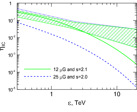
Figure 6: The modification factor $\eta_{\mathrm{ic}}$ in $\gamma$-rays derived from our reference model (lines) and from the data of Acero et al. (2010, shaded regions) for the sets of parameters ($B_{\mathrm{o}}=12{\,\rm\mu G}$, $s=2.1$) and ($B_{\mathrm{o}}=25{\,\rm\mu G}$, $s=2.0$).

4.3 Fit to the TeV $\gamma$-ray spectrum

Fig. 6 compares the modification factors $\eta_{\mathrm{ic}}$ derived from our reference case and from $\gamma$-ray observations. The experimental modification factor $\eta_{\mathrm{\gamma,obs}}$ is calculated from the TeV $\gamma$-ray spectrum $F_{\mathrm{\gamma,obs}}$ of SN 1006 (Acero et al., 2010). It is evaluated as a ratio $\eta_{\mathrm{\gamma,obs}}=F_{\mathrm{\gamma,obs}}/F_{\mathrm{T}}$ of the observed $\gamma$-ray spectrum to the extrapolation of the Thomson IC spectrum to TeV $\gamma$-rays. The latter is found from the radio spectrum as $F_{\mathrm{T}}=\left(F_{\mathrm{T}}/F_{\mathrm{r}}\right)_{\mathrm{theor}}F_{\mathrm{r,obs}}$ where the ratio $\left(F_{\mathrm{T}}/F_{\mathrm{r}}\right)_{\mathrm{theor}}$ is calculated with Eqs. (4) and (7) for $\eta_{\mathrm{syn}}=\eta_{\mathrm{ic}}=1$. Thus,

$$\eta_{\mathrm{\gamma,obs}}=\frac{F_{\mathrm{\gamma,obs}}}{F_{\mathrm{r,obs}}}\frac{C_{\mathrm{r}}\zeta}{C_{\mathrm{T}}\zeta_{\mathrm{T}}}B_{\mathrm{o}}^{(s+1)/2}.$$ (11)

The transformation of the observed TeV spectrum $F_{\mathrm{\gamma,obs}}$ to the modification factor $\eta_{\mathrm{\gamma,obs}}$ depends directly on the magnetic field strength. Note that this is not a new way to estimate the MF strength but just a different representation of the method used by Völk et al. (2008).

The TeV $\gamma$-ray spectrum is almost restored by the pure IC emission in the model with $B_{\mathrm{o}}=12{\,\rm\mu G}$ and $s=2.1$ (Fig. 6 green line). On the contrary, the model with $B_{\mathrm{o}}=25{\,\rm\mu G}$ and $s=2.0$ (which is supported by the X-ray spectrum as well; see Fig. 5) does not agree with the TeV spectrum (Fig. 6 blue line) if only the leptonic $\gamma$-ray emission is considered. Larger values of the MF strength result in the requirement of an additional component to fit the TeV spectrum, as it is the case in the NLA model of Berezhko et al. (2009) or in the mixed or hadronic models of Acero et al. (2010).

Since further in the present paper we consider the pure leptonic model for the TeV $\gamma$-ray emission, we assume $B_{\mathrm{o}}=12{\,\rm\mu G}$. It is worth to note the difference between the spectral index $s_{\mathrm{tot}}=2.1$ derived in this section for SN 1006 as a whole and those derived from the regions covering the remnant edge, and resulting in $s_{\mathrm{loc}}\approx 2.0$ (Miceli et al., 2009).

In Sect. 5, we shall analyse the azimuthal and radial profiles of the surface brightness extracted from regions located quite close to the shock and use $s=2.0$, as suggested by X-ray observations (Miceli et al., 2009). We checked the role of other $s$, and our calculations (not reported here) show that, for $s=2.1$, the profiles of brightness are almost the same as those reported here.

However, our calculations (not reported here) show that, for $s=2.1$, the profiles of brightness are almost the same as those reported here.

5 Constraints from X-ray and gamma-ray maps

5.1 X-ray azimuthal profiles

In Appendix A.1, we demonstrate that the distribution of the surface brightness of a Sedov SNR due to synchrotron emission can be represented as

$$S_{\mathrm{x}}=\mathrm{const}\ {\cal S}_{\mathrm{x}}(\tilde{\nu},\bar{\rho},\varphi;\phi_{\mathrm{o}},b,\epsilon_{\mathrm{f\|}})\ E_{\mathrm{max}}^{1-s}K_{\mathrm{s\|}}B_{\mathrm{o}}R.$$ (12)

The universal shape ${\cal S}_{\mathrm{x}}$ of the radial (for fixed $\varphi$) and azimuthal (for fixed $\bar{\rho}$) profiles is determined just by one parameter, $\epsilon_{\mathrm{f\|}}$, if $s$, $\phi_{\mathrm{o}}$, $b$ as well as the obliquity dependence of the injection efficiency and the model for the maximum energy of electrons are fixed. In case $\epsilon_{\mathrm{f\|}}\gg 1$ and/or $\tilde{\nu}\ll 1$, the role of the radiative losses on the downstream electron distribution is negligible and the profiles of the brightness is then independent on the fiducial energy:

$$S_{\mathrm{x}}=\mathrm{const}\ {\cal S}_{\mathrm{r}}(\bar{\rho},\varphi;\phi_{\mathrm{o}},b)\ \tilde{\nu}^{-(s-1)/2}E_{\mathrm{max}}^{1-s}K_{\mathrm{s\|}}B_{\mathrm{o}}R,$$ (13)

that is the same as Eq. (1) for the radio brightness. On the other hand, our calculations show that the role of the evolution of injection efficiency in time (which is represented by $b$) is less important for X-rays than for the radio because the radiative losses (represented by $\epsilon_{\mathrm{f\|}}$) are dominant in determining the downstream distribution of X-ray emitting electrons.

In our reference model of SN 1006, even $\epsilon_{\mathrm{f\|}}$ is not a free parameter, because it is determined through Eq. (6) by the strength of the MF. Fig. 7 compares theoretical and experimental results. Synthesized azimuthal profiles of the X-ray brightness agree with the observations though the fit is not ideal. Simulations reveal that the strength of the MF is not important for the azimuthal variation of the X-ray brightness.

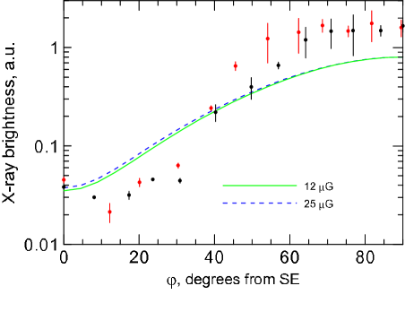
Figure 7: Azimuthal profile of the X-ray brightness at fixed $\bar{\rho}$ which corresponds to the maximum of the radial distribution of brightness at $\varphi=\pi/2$. The calculations are done for $\varepsilon=1.2{\,\rm keV}$, $s=2$ and two values of $B_{\mathrm{o}}$, namely $12{\,\rm\mu G}$ (solid green line) and $25{\,\rm\mu G}$ (dashed blue line). The experimental data are taken from the hard X-ray image of SN 1006 (Miceli et al., 2009). They are derived averaging X-ray brightness along radii within annuli centered on the remnant (from $13.8^{\prime}$ to $14.8^{\prime}$ off the center for SE-NE and from $14.4^{\prime}$ to $15.2^{\prime}$ for SE-SW profile). The profile from SE to SW is in red, that from SE to NE is in black.

Another possibility to change the azimuthal variation of the synchrotron X-ray surface brightness in a model is to consider a broader end of the electron spectrum at the shock, e.g. $N(E)\propto\exp\left(-\left(E/E_{\mathrm{max}}\right)^{\alpha^{\prime}}\right)$. The value $\alpha^{\prime}=0.5\div 0.6$ (Ellison et al., 2000, and references therein) makes the fit even worse. Really, the azimuthal distribution of the brightness is roughly proportional to $\exp\left(-(E_{\mathrm{m}}(\varphi)/E_{\mathrm{max}}(\varphi))^{\alpha^{\prime}}\right)$ where $E_{\mathrm{m}}$ is the energy of electrons which give the largest contribution to emission at an observed frequency. Fig 7 assumes $\alpha^{\prime}=1$; smaller $\alpha^{\prime}$ results in smaller contrasts between azimuth $\varphi=\pi/2$ and $\varphi=0$ that is against of the observations. Larger values of the parameter, $\alpha^{\prime}=1\div 2$, appeared in the loss-limited model (Zirakashvili & Aharonian, 2007; Schure et al., 2010) might increase the contrast but the young age of SN 1006 makes the radiative losses ineffective in limitation of $E_{\mathrm{max}}$.

The differences in the synthesized and observed profiles might be due to nonuniformity of ISMF and/or ISM: larger contrasts of ISMF or ISM density between azimuth $0^{o}$ and $90^{o}$ induced by nonuniformity is obviously able to increase contrasts.

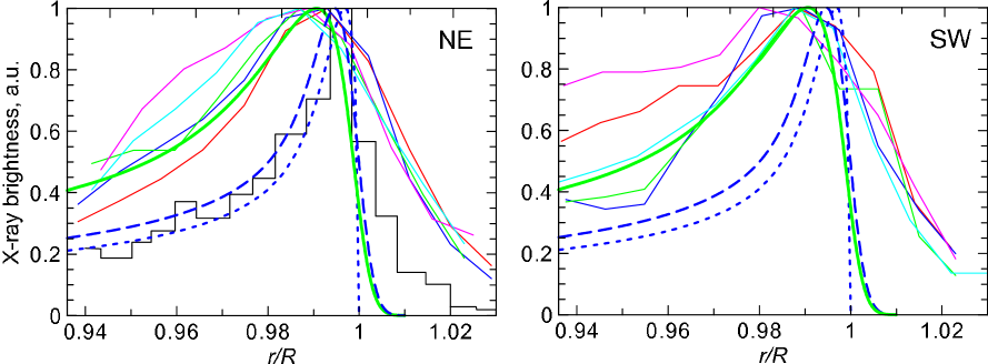
Figure 8: Radial profiles of the X-ray brightness in NE (left) and SW (right) limbs of SN 1006. Experimental XMM-Newton profiles (from regions 1-5 and 6-10 respectively, Fig. 1) for the photon energy range $2\div 4.5{\,\rm keV}$ are in color. The sharpest Chandra radial profile (from Fig. 4A in Long et al., 2003, photon energy is $1.2\div 2{\,\rm keV}$) is shown by the histogram. Theoretical profiles are shown by the thick blue dotted line (for $B_{\mathrm{o}}=25{\,\rm\mu G}$, smoothed to the Chandra resolution by Gaussian with sigma $0.2^{\prime\prime}$), and by the thick green solid line (for $12{\,\rm\mu G}$, smoothed to the XMM resolution by Gaussian with sigma $2.6^{\prime\prime}$). They are calculated at 1.2 keV photons, for azimuth $\varphi=70^{\mathrm{o}}$ in our model of SN 1006, $s=2$. Theoretical profile for $B_{\mathrm{o}}=25{\,\rm\mu G}$ smoothed to the XMM-Newton resolution is shown by the long-dashed blue line.

5.2 X-ray radial profiles

The method for the MF strength estimation from the radial profile of the X-ray brightness is described by Berezhko & Völk (2004) (see also Ballet, 2005). The radiative losses of electrons with energy $E$ is $\dot{E}\propto E^{2}B^{2}$. These losses are less important for electrons emitting in radio but they are able to modify effectively the energy spectrum of electrons radiating X-rays. As a consequence, the synchrotron rim in X-rays is thinner than that in radio. The idea of the method is that the stronger the magnetic field, the larger the radiative energy losses experienced by relativistic electrons. This leads therefore to the rapid decrease of the spatial distribution of electrons behind the shock and to a sharp maximum in the radial X-ray brightness profile. From the observational point of view, the thinner the rim in X-rays the stronger the magnetic field is expected to be.

Fig. 8 compares the theoretical profiles ${\cal S}_{\mathrm{x}}(\bar{\rho})$ with data from XMM and Chandra. The simulated distribution with $B_{\mathrm{o}}=12{\,\rm\mu G}$ (green solid line) fit the XMM data. In our model, the MF compression factor is $\sigma_{\mathrm{B}}=3.8$ at the azimuth $\varphi=70^{\mathrm{o}}$. The post-shock MF is therefore $B_{\mathrm{s}}\simeq 45{\,\rm\mu G}$ in both NE and SW limbs. This value could be considered as an upper limit for an average MF within the limbs because some observed profiles are a bit thicker than the theoretical one which is shown by the thick green line. The strength $B_{\mathrm{o}}=25{\,\rm\mu G}$ (long-dashed blue line) does not fit XMM the radial profiles of X-ray brightness.

However, the sharpest Chandra profile (Fig. 4A in Long et al., 2003) may not be explained by $B_{\mathrm{s}}\simeq 45{\,\rm\mu G}$. Our model fits this profile if the post-shock field is $B_{\mathrm{s}}\simeq 95{\,\rm\mu G}$ (blue dotted line). The same filament was used by Berezhko et al. (2003) to deduce $\simeq 130{\,\rm\mu G}$ field. Our estimate for the thinnest filament is comparable but lower than in the NLA model. The reasons of such discrepancy are some differences between our and their models. Namely, in our model, MF decreases downstream of the shock while the extreme NLA model assumes uniform MF. In addition, we accept (following Reynolds, 1998) that accelerated electrons are confined in the fluid element while Berezhko et al. (2003) include diffusion.

In general, MF estimated from the radial profile of X-ray brightness reflects the local conditions. The quite large strength of the downstream magnetic field, $B\simeq 130-150{\,\rm\mu G}$, adopted in the extreme NLA model, was assumed to be the same everywhere in the SN 1006 interior (Berezhko et al., 2009). This value is reasonable for a thinnest NE filament (Fig. 4A in Long et al., 2003) as it is apparent from the fitting of the radial profile of X-ray brightness (Berezhko et al., 2003; Ksenofontov et al., 2005). However, the two close radial profiles are already thicker (Fig. 4B,C in Long et al., 2003) suggesting therefore a smaller value of $B$ even around the location of the original sharpest filament.

An effective MF inside SN 1006 (i.e. which may be used to represent SNR as a whole) is smaller. Let us consider two possible effective field values: the volume average

$$\left\langle B\right\rangle_{\mathrm{v}}=V^{-1}{\int BdV}$$ (14)

and the radio-emissivity weighted volume average

$$\left\langle B\right\rangle_{\mathrm{ev}}=\int BPdV\Big{/}\int PdV.$$ (15)

(The radio-emissivity weighted volume average is higher than the volume average because the emissivity $P$ quickly decreases downstream; thus, in calculation of the average, most of the contribution comes from regions close to the shock where the MF is large.) It may easily be shown analytically that (due to self-similarity of the Sedov solution) both $\left\langle B\right\rangle_{\mathrm{v}}$ and $\left\langle B\right\rangle_{\mathrm{ev}}$ are simply products of $B_{\mathrm{o}}$ and some constants. Our model predicts $B_{\mathrm{o}}=12{\,\rm\mu G}$ and yields $\left\langle B\right\rangle_{\mathrm{v}}=1.06B_{\mathrm{o}}=12{\,\rm\mu G}$ and $\left\langle B\right\rangle_{\mathrm{ev}}=2.7B_{\mathrm{o}}=32{\,\rm\mu G}$. The latter is in good agreement with the strength ($\approx 30{\,\rm\mu G}$) found in the leptonic model of Acero et al. (2010) and with the estimation (again $\approx 30{\,\rm\mu G}$) derived from Fig. 1 in Völk et al. (2008) with the use of the HESS spectrum.

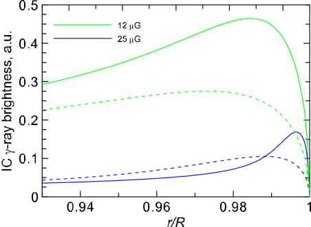
Figure 9: Radial profiles of the IC $\gamma$-ray brightness at 1 TeV in our model of SN 1006, for azimuth $\varphi=0$ (dotted lines) and $\varphi=\pi/2$ (solid lines), for two values of $B_{\mathrm{o}}$; $\phi_{\mathrm{o}}=70^{\mathrm{o}}$, $s=2$.

5.3 A note on the gamma-ray brightness

The distribution of the IC brightness in $\gamma$-rays with energies $\varepsilon$ is given by (Appendix A.2)

$$S_{\mathrm{ic}}=\mathrm{const}\ {\cal S}_{\mathrm{ic}}(\varepsilon,\bar{\rho},\varphi;\phi_{\mathrm{o}},b,\epsilon_{\mathrm{f\|}},E_{\mathrm{max}})\ K_{\mathrm{s\|}}R.$$ (16)

This formula shows which factors affect the shape of the azimuthal and radial profiles and which determine their amplitudes. The $\gamma$-ray image of SN 1006 (namely, the shapes ${\cal S}$ of the azimuthal and radial profiles in these bands) – like the X-ray map – depend only on the value of $B_{\mathrm{o}}$, once other parameters are fixed.

SN 1006 is rather faint in TeV $\gamma$-rays to allow, at present time, to derive azimuthal and radial profiles with quality comparable to those obtained in the radio and X-ray bands. However, we may check whether our model provides the observed location of the bright $\gamma$-ray limbs. Fig. 9 shows the radial profiles of the $\gamma$-ray surface brightness in our model of SN 1006. The bright limbs are located at the azimuth $\varphi=\pi/2$ for both strengths of MF considered (namely, $12$ and $25\mu$G), in agreement with the observations. Note that such property is not universal; it depends on the parameters of the model. For example, if an aspect angle would be $90^{\mathrm{o}}$ then the observed location of the TeV $\gamma$-ray limbs may be possible only for ISMF strength larger than $\sim 100{\,\rm\mu G}$. We address this issue in a separate paper.

6 Discussion and Conclusions

The magnetic field strength in SN 1006 is one of the key parameter in the model. Being related to $E_{\mathrm{max\|}}$ with Eq. (3) and to the parameter $\epsilon_{\mathrm{f\|}}$ (which regulates efficiency of the radiative losses of relativistic electrons) with Eq. (6), it influences almost everything in nonthermal spectra and images.

Table 1: Summary of the observables used for parameter determination and cross-check^a

Observable	Parameter	Value
radio azumuthal profileb	aspect angle	$\phi_{\mathrm{o}}=70^{\mathrm{o}}\pm 4.2^{\mathrm{o}}$
	injection type	isotropic
	orientation of ISMF and SNR morphology	SE-NW, barrel-like
radio radial profile	$b$ in $K_{\mathrm{s}}\propto V^{-b}$	$-1\;\lower 4.0pt\hbox{${\buildrel\displaystyle<\over{\sim}}$}\,b\;\lower 4.0pt\hbox{${\buildrel\displaystyle<\over{\sim}}$}\,0$
local broad-band fits of spectrac	local index $s_{\mathrm{loc}}$ over shock	$s_{\mathrm{loc}}=2.0$ over most of SNR rim
$\nu_{\mathrm{break}}$ azimuthal profilec	model of $E_{\mathrm{max}}$	time-limitedd
	ratio of the mean free path to Larmour radius	$\eta=1.5$
	electron maximum energy at parallel shock	$E_{\mathrm{max\|}}=7.0(B_{\mathrm{o}}/12{\,\rm\mu G})^{-1/2}{\,\rm TeV}$
	electron maximum energy at perpendicular shock	$E_{\mathrm{max\bot}}=3.25E_{\mathrm{max\|}}$
radio and hard X-ray spectrum	MF strength and index $s_{\mathrm{tot}}$ for the whole SNR	($B_{\mathrm{o}}=25{\,\rm\mu G}$ and $s_{\mathrm{tot}}=2.0$) or
		($B_{\mathrm{o}}=12{\,\rm\mu G}$ and $s_{\mathrm{tot}}=2.1$)
radio and TeV $\gamma$-ray spectrum	$\gamma$-ray emission model, MF strength and index $s_{\mathrm{tot}}$	IC with $B_{\mathrm{o}}=12{\,\rm\mu G}$ and $s_{\mathrm{tot}}=2.1$
X-ray radial profiles	post-shock MF strength in the limbs	$B_{\mathrm{s\bot}}\simeq 50{\,\rm\mu G}$
X-ray azimuthal profile	MF strength	OK
	ISMF orientation and aspect angle	OK
	model of $E_{\mathrm{max}}$	OK
$\gamma$-ray limbs location	MF strength, aspect angle	OK
	$\gamma$-ray emission model	OK
a the model assumes uniform ISMF/ISM and $\gamma=5/3$
b Petruk et al. (2009c); Schneiter et al. (2010)
c Miceli et al. (2009)
d see also Katsuda et al. (2010)

We consider a ‘classic’ model of SN 1006, i.e. model which is based on classic MHD and acceleration theories. Since they are better developed compared to NLA approach, they allow us to put observational constraints on the (test-particle) kinetics and MF, to compare the azimuthal variations of the electron maximum energy and the surface brightness in radio, hard X-rays and TeV $\gamma$-rays. At the present time, such comparison may not be done in the frame of the NLA theory. We demonstrate that the ‘classic’ model is in agreement with most of the observational data.

We try to fix free parameters of the model step-by-step, looking for observations which is mostly sensitive to some of them (Table 1). In addition to the commonly used broad-band spectrum, the properties of the nonthermal (radio, X-ray and TeV $\gamma$-ray) images of SNR as well as spatially resolved spectral fits are considered.

In particular, the morphology and azimuthal profiles of the radio brightness may determine the orientation of ISMF. Namely, the radio data may be fitted by the model with uniform ISMF which is oriented perpendicular to the Galactic plane with an angle $70^{\mathrm{o}}$ to the line of sight (Petruk et al., 2009c; Schneiter et al., 2010). If so, the injection efficiency should be independent of obliquity. The radial distribution of the radio brightness depends now only on the way the injection efficiency varies with time ($K\propto V^{-b}$). The observations however may not definitively fix $b$. It is somewhere between $-1$ and $0$ but accuracy of the data allow also for a bit wider range. Spatially resolved X-ray analysis of regions around the forward shock demonstrate that distribution of $\nu_{\mathrm{break}}$ may be explained by the time-limited model of $E_{\mathrm{max}}$; this is in agreement with recent results of Katsuda et al. (2010). The maximum energy of electrons at the parallel shock is found $E_{\mathrm{max\|}}=7(B_{\mathrm{o}}/12{\,\rm\mu G})^{-1/2}{\,\rm TeV}$. It is 3.25 times higher at regions where shock is perpendicular.

We obtain expressions for the radio, X-ray and $\gamma$-ray spectra from the whole SNR in a form which clearly show which parameter of the model is responsible for the amplitude of the spectrum and which one for its shape. The modification factor of the synchrotron X-ray spectrum – which shows the deviation of the spectrum from the power law – may well be explained by the classical model with ISMF strength $B_{\mathrm{o}}=25{\,\rm\mu G}$ if $s=2.0$ or with $B_{\mathrm{o}}=12{\,\rm\mu G}$ if $s=2.1$. At the same time, the TeV $\gamma$-ray modification factor prefers only the pair $B_{\mathrm{o}}=12{\,\rm\mu G}$, $s=2.1$; TeV emission is then completely due to IC process. In case $B_{\mathrm{o}}=25{\,\rm\mu G}$, an additional component in the TeV $\gamma$-ray spectrum is needed, from pion decays, as it is in the model of Berezhko et al. (2009). The proton injection in such scenario should increase with obliquity in order to fit the observed azimuthal profiles of TeV $\gamma$-ray brightness (ISMF is parallel to the limbs). Could the electron and proton injections have so different dependences on obliquity in the same SNR: isotropic for electrons and quasi-perpendicular for protons?

The extreme NLA approach (Berezhko et al., 2009) predicts $B_{\mathrm{o}}=30{\,\rm\mu G}$ immediately before the forward shock and $B=150{\,\rm\mu G}$ everywhere inside the SNR. A number of the radial profiles of X-ray brightness obtained from XMM image agree with our model if an ambient MF is $B_{\mathrm{o}}=12{\,\rm\mu G}$. Around the quasi-perpendicular shock, where the profiles are extracted from, our model predicts the post-shock MF with strength $B_{\mathrm{s\bot}}\simeq 50{\,\rm\mu G}$. However, in the classic model of SN 1006, this is the value immediately post-shock; after then it rapidly decreases downstream. Therefore, an effective (emissivity weighted average) MF within SN 1006 is estimated to be $32{\,\rm\mu G}$ that agrees well with estimates of Völk et al. (2008) and Acero et al. (2010). MF in the sharpest Chandra profile is fitted in our model with $B_{\mathrm{s}}=95{\,\rm\mu G}$; it reflects the local conditions, only within this filament.

We found that the broad-band spectrum from the whole SN 1006 is better represented with the electron spectral index $s_{\mathrm{tot}}=2.1$ while local radio-to-X-ray spectra over the SNR shock prefers $s_{\mathrm{loc}}=2.0$ (Miceli et al., 2009). It is interesting, that similar difference in spectral index is found in the theoretical study of Schure et al. (2010): the spectrum near the shock is flatter than the overall spectrum. The authors attributed this difference to the time evolution of $E_{\mathrm{max}}$ which was lower at previous times. In contrast, the time-limited model for the maximum energy (Reynolds, 1998) which fits the azimuthal variation of $\nu_{\mathrm{break}}$ in SN 1006 (Sect. 3) as well as absence of the time variation of the synchrotron flux (Katsuda et al., 2010), suggest what $E_{\mathrm{max}}$ varies quite slowly in this SNR, at least in the regions close to the shock. The issue of different spectral slopes has to be considered in the future. As to the purpose of the present study, difference between $s_{\mathrm{tot}}$ and $s_{\mathrm{loc}}$ is negligible for azimuthal and radial profiles of radio, X-ray and IC $\gamma$-ray brightness.

Azimuthal profiles of the X-ray and $\gamma$-ray brightness in our model behave in the same way as in the observations.

‘Classic’ model has also few difficulties. Rothenflug et al. (2004) developed a simple geometrical criterion to distinguish between barrel-like and polar-cap morphology in SN 1006. They have shown analytically that the ratio between the central and the rim brightness should be larger than some value in BarMF case (projected “barrel” has to provide enough brightness in the internal regions). In XMM map, this ratio is smaller. The luck of brightness from equatorial belt in the central part is an argument against BarMF morphology. Our model, which strongly prefer BarMF, does not agree with the criterion of Rothenflug et al. (2004). Nevertheless, the polar-cap scenario, which is in agreement with this criterion (and is adopted by the NLA model), is unable to explain the observed azimuthal profiles of the break frequency $\nu_{\mathrm{break}}$and the radio brightness, under assumptions that ISMF/ISM are uniform and the amplified/compressed MF increases with obliquity.

Another minor point of the classic model of SN 1006 is the rather large ambient MF, $B_{\mathrm{o}}=12{\,\rm\mu G}$, which is difficult to expect without MF amplification at the high location of SN 1006 above the Galactic plane.

Our model deals with ideal gas with the adiabatic index $\gamma=5/3$ and cannot explain the small distance between the forward shock and the contact discontinuity (Cassam-Chenaï et al., 2008; Miceli et al., 2009). Instead, if acceleration is so efficient that relativistic particles affect hydrodynamics then the adiabatic index may be smaller than ours. The small distance observed may naturally be explained by such, more compressible, plasma with the index like $\gamma=1.1$ (Orlando et al., 2010). It is worth noting that in such case of efficient acceleration, there is no need for MF amplification: the only shock compression to factor $\sigma=21$ (as it is for $\gamma=1.1$) may result in quite large downstream MF even in case of $B_{\mathrm{o}}$ of few ${\,\rm\mu G}$.

The two models, classical and extream NLA, are compared in Table 2. It is evident that none of them explaine the whole set of the SN 1006 properties. A new model of SN 1006 has to include either combination of the two extremes or inclusion of the ISMF/ISM nonuniformity.

All results presented here are obtained under assumption that SN 1006 evolve in the uniform ISMF and uniform ISM. It is shown that the scenario of classic MHD/acceleration plus uniform ISMF/ISM strongly prefers the barell-like morphology of SN 1006. However, we also see that nonuniform ISMF/ISM could be an essential element in the model of SN 1006. In particular, slanted lobes, the inversion of the brightness ratio between NE and SW limbs from radio to X-ray band and the higher break frequency in NE limb may only be explained by presence of gradient of ISMF and/or ISM. We expect that the effect of the nonuniform ISMF might dominate the role of some nonlinear effects arising from efficient acceleration of cosmic rays by the forward shock in SN 1006. We like to address this issue in the future.

Table 2: Comparison of SN 1006 models

Properties of SN 1006	Classic modela	Extream NLA modelb
	(with uniform ISMF)	(with uniform ISMF)
two-limbs in radio and hard X-ray image	YES	YES?
	SN 1006 is barrel	SN 1006 has polar caps
	ISMF direction: SE-NW	ISMF direction: SW-NE
location of TeV $\gamma$-ray limbs	YES	YES?
Rothenflug et al. (2004) criterion	NO	YES
radio spectrum	YES as power low	YES with concave shape
hard X-ray spectrum	YES with $\left\langle B\right\rangle_{\mathrm{ev}}=32{\,\rm\mu G}$	YES with $\left\langle B\right\rangle_{\mathrm{v}}\approx 150{\,\rm\mu G}$
TeV $\gamma$-ray spectrum	YES	YES
	IC with $\left\langle B\right\rangle_{\mathrm{ev}}\approx 32{\,\rm\mu G}$	IC with $\left\langle B\right\rangle_{\mathrm{v}}\approx 150{\,\rm\mu G}$
		and hadronic component
radio radial profile	YES	NO? (uniform $B$ inside SNR)
sharpest X-ray radial profile	YES with $B_{\mathrm{s}}\approx 95{\,\rm\mu G}$	YES with $B_{\mathrm{s}}\approx 150{\,\rm\mu G}$
radio azimuthal profile	YES	?
hard X-ray azimuthal profile	YES	?
TeV $\gamma$-ray azimuthal and radial profiles	YES	?
$\nu_{\mathrm{break}}$ azimuthal profiles	YES	NO?
pre-shock MF strength $B_{\mathrm{o}}=12{\,\rm\mu G}$	NO	YES
	(if ISMF around SN 1006	as result of amplification
	is typical $\sim 3{\,\rm\mu G})$	(if any)
(eventual) concave shape of the radio spectrumc	NO	YES
very close forward shock and contact discontinuity	NO	YES (with $\gamma=1.1$)
radio ‘overbrightness’ in the SNR interior	NO	NO?
slanted lobes	NO	NO
ratio of radio ${\cal R}_{\mathrm{r}}<1$ and X-ray brightness ${\cal R}_{\mathrm{x}}>1$	NO	NO
$\nu_{\mathrm{break,NE}}/\nu_{\mathrm{break,SW}}>1$	NO	NO
a present paper
b Berezhko et al. (2009)
c Allen et al. (2008)

Appendix A Surface brightness of Sedov SNR

Surface brightness of a spherical SNR is an integral of volume emissivity $q$ along the line of sight

$$S_{\mathrm{syn}}=2\int\limits_{0}^{R}qdl=2R\int\limits_{\bar{a}(\bar{\rho})}^{1}q\frac{\bar{r}\bar{r}_{\bar{a}}d\bar{a}}{\sqrt{\bar{r}^{2}-\bar{\rho}^{2}}},$$ (17)

where $\rho$ is distance from the center of projection, $\bar{r}=r/R$, $a$ Lagrangian coordinate, $r_{a}=dr/da$,

$$q=\int N(E)p(E,\varepsilon)dE,$$ (18)

where $E$ and $\varepsilon$ are the electron and photon energies, $p$ the radiation power of a single electron. In case of Sedov SNR in uniform medium the electron energy distribution downstream of the shock is (Petruk & Beshley, 2008)

$$N(E)=KE^{-s}{\cal E}_{\mathrm{rad}}^{s-2}\exp\left(-\frac{E}{E_{\mathrm{max\|}}{\cal E}_{\mathrm{ad}}{\cal E}_{\mathrm{rad}}f_{\mathrm{E}}}\right),$$ (19)

the normalization $K=K_{\mathrm{s\|}}(t)f_{\mathrm{K}}(\Theta_{\mathrm{o}})\bar{K}(\bar{a})$, the magnetic field $B=B_{\mathrm{s\|}}(t)\sigma_{\mathrm{B}}(\Theta_{\mathrm{o}})\bar{B}(\bar{a})$ and the electron maximum energy $E_{\mathrm{max}}=E_{\mathrm{max\|}}f_{\mathrm{E}}(\Theta_{\mathrm{o}})$.

A.1 Synchrotron emission

The synchrotron radiation power is

$$p=\frac{\sqrt{3}e^{3}\left\langle\sin\phi\right\rangle}{m_{\mathrm{e}}c^{2}}BF_{\mathrm{syn}}\left(\frac{\nu}{\nu_{\mathrm{c}}}\right),$$ (20)

where all notations have their common meaning. The synchrotron surface brightness of Sedov SNR is therefore

$$S_{\mathrm{syn}}=\frac{2\sqrt{3}e^{3}\left\langle\sin\phi\right\rangle}{m_{\mathrm{e}}c^{2}}{\cal S}_{\mathrm{syn}}(\tilde{\nu},\bar{\rho},\varphi;\phi_{\mathrm{o}},b,\epsilon_{\mathrm{f\|}})\ E_{\mathrm{max}}^{1-s}K_{\mathrm{s\|}}B_{\mathrm{o}}R.$$ (21)

where ${\cal S}_{\mathrm{syn}}(\tilde{\nu},\bar{\rho},\varphi)$ is a universal dimensionless function

$$\begin{array}[]{l}\displaystyle{\cal S}_{\mathrm{syn}}=\int\limits_{\bar{a}(\bar{\rho})}^{1}\left[\int\limits_{0}^{\infty}F_{\mathrm{syn}}\left(\frac{\tilde{\nu}}{\epsilon^{2}\sigma_{\mathrm{B}}\bar{B}}\right)\epsilon^{-s}{\cal E}_{\mathrm{rad}}^{s-2}\right.\\ \\ \displaystyle\qquad\qquad\times\left.\exp\left(-\frac{\epsilon}{{\cal E}_{\mathrm{ad}}{\cal E}_{\mathrm{rad}}f_{\mathrm{E}}}\right)d\epsilon\right]\\ \\ \displaystyle\qquad\qquad\times\sigma_{\mathrm{B}}\bar{B}f_{\mathrm{K}}\bar{K}\frac{\bar{r}\bar{r}_{\bar{a}}d\bar{a}}{\sqrt{\bar{r}^{2}-\bar{\rho}^{2}}},\end{array}$$ (22)

where $\epsilon=E/E_{\mathrm{max\|}}$. It depends on the dimensionless models of obliquity variations of $K$, $B$ and $E_{\mathrm{max}}$ (i.e. on $f_{\mathrm{K}}$, $\sigma_{\mathrm{B}}$, $f_{\mathrm{E}}$) but is independent of the actual values of $E_{\mathrm{max}}$, $K_{\mathrm{s}}$, $B_{\mathrm{o}}$ and $R$.

In the limit $\epsilon_{\mathrm{f\|}}\gg 1$ and/or $\tilde{\nu}\ll 1$, Eq. (21) transforms to

$$\begin{array}[]{l}S_{\mathrm{syn}}=\displaystyle\frac{2\sqrt{3}e^{3}\left\langle\sin\phi\right\rangle{\cal A}(s)}{m_{\mathrm{e}}c^{2}}\ {\cal S}_{\mathrm{r}}(\bar{\rho},\varphi;\phi_{\mathrm{o}},b)\\ \\ \qquad\times\ {\tilde{\nu}}^{-(s-1)/2}E_{\mathrm{max}}^{1-s}K_{\mathrm{s\|}}B_{\mathrm{o}}R.\end{array}$$ (23)

where

$${\cal S}_{\mathrm{r}}=\int\limits_{\bar{a}(\bar{\rho})}^{1}\left(\sigma_{\mathrm{B}}\bar{B}\right)^{(s+1)/2}f_{\mathrm{K}}\bar{K}\frac{\bar{r}\bar{r}_{\bar{a}}d\bar{a}}{\sqrt{\bar{r}^{2}-\bar{\rho}^{2}}},$$ (24)

or, in other form,

$$\begin{array}[]{l}S_{\mathrm{r}}=\displaystyle\frac{2\sqrt{3}e^{3}\left\langle\sin\phi\right\rangle{\cal A}(s)}{m_{\mathrm{e}}c^{2}}\ {\cal S}_{\mathrm{r}}(\bar{\rho},\varphi;\phi_{\mathrm{o}},b)\\ \\ \qquad\times\ \left(\nu/c_{1}\right)^{-(s-1)/2}K_{\mathrm{s\|}}B_{\mathrm{o}}^{(s+1)/2}R.\end{array}$$ (25)

A.2 IC emission

The IC radiation power is

$$p=\frac{2e^{4}m_{\mathrm{e}}^{2}c^{2}kT}{\pi\hbar^{3}}E^{-2}{\cal I}(E,\varepsilon),$$ (26)

where all notations have their common meaning, ${\cal I}$ is a special integral (see e.g. Petruk, 2008). The IC brightness is therefore

$$S_{\mathrm{ic}}=\frac{4e^{4}m_{\mathrm{e}}^{2}c^{2}kT}{\pi\hbar^{3}}\ {\cal S}_{\mathrm{ic}}(\varepsilon,\bar{\rho},\varphi;\phi_{\mathrm{o}},b,\epsilon_{\mathrm{f\|}},E_{\mathrm{max}})\ K_{\mathrm{s\|}}R.$$ (27)

The function ${\cal S}_{\mathrm{ic}}(\bar{\rho},\varphi)$ is not so universal as in case of the synchrotron emission; it depends on the absolute values of the photon energy and the maximum electron energy; we do not present it here.

Appendix B Nonthermal spectrum of Sedov SNR

Flux is defined as

$$F(\nu)=\left(4\pi d^{2}\right)^{-1}\int P(\nu)dV$$ (28)

where $V$ is the volume of SNR and $P$ the volume emissivity. We assume that the energy spectrum of electrons in the form

$$N(E)dE=KE^{-s}\exp(-E/E_{\mathrm{max}})dE$$ (29)

are created at the shock. The volume emissivity is

$$P(\nu)=\int N(E)p(E,\nu)dE$$ (30)

where $p$ is the spectral distribution of radiation power of ‘single’ electron with energy $E$. Let us consider adiabatic SNR in uniform ISM and uniform ISMF.

In general, the efficiency of injection may depend on the shock obliquity angle $\Theta_{\mathrm{o}}$. If particles are injected easier at quasiparallel shocks then $K_{\mathrm{s}}(\Theta_{\mathrm{o}})$ is decreasing function of $\Theta_{\mathrm{o}}$ with decrement rate dependent on the level of turbulence, shock strength etc. (Ellison et al., 1995). Let us consider parametric representation $K_{\mathrm{s}}=K_{\mathrm{s\|}}f_{\mathrm{K}}(\Theta_{\mathrm{o}})$ with approximation $f_{\mathrm{K}}=\exp\left(-\left(\Theta_{\mathrm{o}}/\Theta_{\mathrm{K}}\right)^{2}\right)$ where $K_{\mathrm{s\|}}$ the normalization for region immediately after the parallel shock, $\Theta_{\mathrm{K}}$ the parameter. $\Theta_{\mathrm{K}}=\pi/6$ approximates the classical quasiparallel dependence, $\varsigma\propto\cos^{2}(\Theta_{\mathrm{o}})$. In case of the isotropic injection, $\Theta_{\mathrm{K}}=\infty$.

Figure 10: $\zeta$ for different values of parameters $b$ and $\Theta_{\mathrm{K}}$. $s=2$

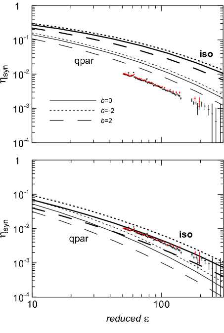
Figure 11: Modification factor $\eta_{\mathrm{syn}}$. Calculations are done for $s=2$, the time-limited model of $E_{\mathrm{max}}$ with $\eta=1.5$, isotropic injection (thick lines) and quasiparallel injection (thin lines), three values of $b$, $\epsilon_{\mathrm{f\|}}=100$ (upper panel) and $\epsilon_{\mathrm{f\|}}=3.2$ (lower panel). Experimental modification factor for SN 1006 are shown for comparison. It is obtained from the SUZAKU spectrum (Bamba et al., 2008, Fig. 6) for photon energies $\geq 2{\,\rm keV}$, with the use of Eq. (10). MF strength is given by Eq. (6): $B_{\mathrm{o}}=3{\,\rm\mu G}$ (upper panel) and $B_{\mathrm{o}}=30{\,\rm\mu G}$ (lower panel).

B.1 Synchrotron emission

The radio flux (28) from Sedov SNR may be written as (for details, see Petruk & Beshley, 2007)

$$F_{\mathrm{r}}(\nu)=C\nu^{-(s-1)/2}\zeta(b,\Theta_{\mathrm{K}})K_{\mathrm{s\|}}B_{\mathrm{o}}^{(s+1)/2}R^{3}d^{-2}$$ (31)

where

$$C={(4\pi)^{-1}}{{\cal A}(s)c_{2}\mu_{\mathrm{\phi}}c_{1}^{(s-1)/2}},$$ (32)

$c_{1}=3e/(4\pi m_{\mathrm{e}}^{3}c^{5})$, $c_{2}=\sqrt{3}e^{3}/(m_{\mathrm{e}}c^{2})$,

$${\cal A}(s)=\frac{2^{(s-1)/2}}{s+1}\Gamma\left(\frac{3s+19}{12}\right)\Gamma\left(\frac{3s-1}{12}\right),$$ (33)

$\mu_{\mathrm{\phi}}=\left\langle\sin(\varphi)^{(s+1)/2}\right\rangle$, ($C=3.493\times 10^{-14}{\,\rm cgs}$ in case $s=2$), $\varphi$ the angle between MF and the line of sight,

$$\zeta(b,\Theta_{\mathrm{K}})=\int\limits_{0}^{2\pi}\!d\varphi\!\int\limits_{0}^{\pi}\!\!d\theta\sin\theta f_{\mathrm{K}}\!\int\limits_{0}^{1}\!\!d\bar{a}\bar{r}^{2}\bar{r}_{\mathrm{\bar{a}}}\bar{K}\!\left(\sigma_{\mathrm{B}}\bar{B}\right)^{(s+1)/2}\!\!,$$ (34)

$\sigma_{\mathrm{B}}(\Theta_{\mathrm{o}})$ is the compression factor for MF, $r$ and $a$ are Eulerian and Lagrangian coordinates respectively, $r_{\mathrm{a}}=dr/da$, bar represents parameter divided by its post-shock value, $(\varphi,\theta)$ spherical coordinates. Thanks to the self-similarity, the constant $\zeta$ ‘compactifies’ the whole downstream evolution of fluid elements (Sedov, 1959), magnetic field and relativistic electrons (Reynolds, 1998).

In a similar fashion, the X-ray flux is (Petruk & Beshley, 2008)

$$F_{\mathrm{x}}(\tilde{\nu})=C_{2}\zeta_{\mathrm{x}}(\tilde{\nu};b,\Theta_{\mathrm{K}},\epsilon_{\mathrm{f\|}})K_{\mathrm{s\|}}B_{\mathrm{o}}E_{\mathrm{max\|}}^{1-s}R^{3}d^{-2}$$ (35)

where $\tilde{\nu}=\nu/\nu_{\mathrm{c}}(E_{\mathrm{max\|}},B_{\mathrm{o}})$, $\nu_{\mathrm{c}}(E,B)\propto E^{2}B$ is the synchrotron characteristic frequency, $C_{2}=c_{2}\left\langle\sin\varphi\right\rangle/(4\pi)$ a constant, $\epsilon_{\mathrm{f\|}}=637\left(B_{\mathrm{s\|}}^{2}tE_{\mathrm{max\|}}\right)^{-1}$ is the reduced fiducial energy. The energy $\epsilon_{\mathrm{f}}$ is a measure of importance of radiative losses in modification of the electron spectrum (Reynolds, 1998). The function

$$\begin{array}[]{l}\zeta_{\mathrm{x}}(\tilde{\nu};b,\Theta_{\mathrm{K}},\epsilon_{\mathrm{f\|}})=\displaystyle\int\limits_{0}^{2\pi}\!d\varphi\!\int\limits_{0}^{\pi}\!\!d\theta\sin\theta f_{\mathrm{K}}\!\int\limits_{0}^{1}\!\!d\bar{a}\bar{r}^{2}\bar{r}_{\mathrm{\bar{a}}}\bar{K}\sigma_{\mathrm{B}}\bar{B}\!\\ \\ \quad\times\displaystyle\int\limits_{0}^{\infty}\!d\epsilon\epsilon^{-s}{\cal E}_{\mathrm{rad}}^{s-2}\exp\left(-\frac{\epsilon}{{\cal E}_{\mathrm{ad}}{\cal E}_{\mathrm{rad}}f_{\mathrm{E}}}\right)F_{\mathrm{syn}}\left(\frac{\tilde{\nu}}{\epsilon^{2}\sigma_{\mathrm{B}}\bar{B}}\right),\end{array}\!\!\!\!\!$$ (36)

where ${\cal E}_{\mathrm{ad}}(a)$, ${\cal E}_{\mathrm{rad}}(a;\epsilon_{\mathrm{f\|}},\Theta_{\mathrm{o}})$ represent adiabatic and radiative losses of relativistic electrons (Petruk & Beshley, 2008), $F_{\mathrm{syn}}$ the function known in the theory of synchrotron radiation, $\epsilon=E/E_{\mathrm{max\|}}$.

With $\tilde{\nu}$, the radio flux (31) may be written in a form similar to (35):

$$F_{\mathrm{r}}(\tilde{\nu})=C_{2}{\cal A}(s)\tilde{\nu}^{-(s-1)/2}\zeta(b,\Theta_{\mathrm{K}})K_{\mathrm{s\|}}B_{\mathrm{o}}E_{\mathrm{max\|}}^{1-s}R^{3}d^{-2}.$$ (37)

Comparison of (35) and (37) demonstrates that, for $\nu$ much smaller than X-ray frequencies, $\zeta_{\mathrm{x}}$ transforms to $\zeta$, as expected:

$$\zeta_{\mathrm{x}}(\tilde{\nu})={\cal A}(s)\ \tilde{\nu}^{-(s-1)/2}\zeta.$$ (38)

This transition may also be shown analytically from (36), in the limit $E\ll E_{\mathrm{max}}$ and $E\ll\epsilon_{\mathrm{f}}E_{\mathrm{max}}$ (Petruk & Beshley, 2008).

Let us introduce the modification factor for the synchrotron spectrum

$$\eta(\tilde{\nu},\epsilon_{\mathrm{f\|}})=\frac{\zeta_{\mathrm{x}}(\tilde{\nu},\epsilon_{\mathrm{f\|}})\tilde{\nu}^{(s-1)/2}}{{\cal A}(s)\zeta}.$$ (39)

It is defined to be $\eta\leq 1$ and ensure $\eta\rightarrow 1$ for $\nu\ll\nu_{\mathrm{c}}(E_{\mathrm{max\|}},B_{\mathrm{o}})$, as it is given by (38). In terms of $\tilde{\nu}$, the modification factor is almost universal (i.e. allows for scaling with frequency).

With the modification factor, the expression (35) which describes the broad-band (radio-to-X-ray) synchrotron spectrum from Sedov SNR becomes

$$F(\nu)=C\nu^{-(s-1)/2}\zeta(b,\Theta_{\mathrm{K}})\eta(\tilde{\nu};\epsilon_{\mathrm{f\|}})K_{\mathrm{s\|}}B_{\mathrm{o}}^{(s+1)/2}R^{3}d^{-2}.$$ (40)

The values of $\zeta$ are shown on Fig. 10. The parameter $\zeta$ is important in normalization of synchrotron spectrum: it varies in about 8 times over the parameter space. If injection is considerably larger at parallel shocks ($\Theta_{\mathrm{K}}\leq\pi/3$), the value of $b$ is almost unimportant for amplitude of the synchrotron spectrum, but rather small changes in $\Theta_{\mathrm{K}}$ may cause differences in $\zeta$ in few times. In contrast, if injection tends to be isotropic ($\Theta_{\mathrm{K}}\geq 2\pi/3$), $b$ plays the dominant role.

In order to explore the parameter space, we made several runs to calculate the modification factors for different sets of parameters. Results are shown on Fig. 11 where we also plot the experimental data in order to demonstrate relevance of the parameters for SN 1006. The modification factor depends on $\epsilon_{\mathrm{f\|}}$, $b$, $\Theta_{\mathrm{K}}$ and $s$ as well as on the function $f_{\mathrm{E}}(\Theta_{\mathrm{o}})$.

B.2 Inverse-Compton emission

The inverse-Compton flux (28) from electrons in a black-body photon field with temperature $T_{\mathrm{CMB}}$, at photon energies far below TeV (i.e. when the Thomson regime and power-law electron distribution are assumed, see Petruk (2008) for details), is

$$F_{\mathrm{T}}(\varepsilon)=C_{\mathrm{T}}\varepsilon^{-(s-1)/2}\zeta_{\mathrm{T}}(b,\Theta_{\mathrm{K}})K_{\mathrm{s\|}}R^{3}d^{-2}$$ (41)

where $\varepsilon$ is the photon energy,

$$\zeta_{\mathrm{T}}(b,\Theta_{\mathrm{K}})=\int\limits_{0}^{2\pi}\!d\varphi\!\int\limits_{0}^{\pi}\!\!d\theta\sin\theta f_{\mathrm{K}}\!\int\limits_{0}^{1}\!\!d\bar{a}\bar{r}^{2}\bar{r}_{\mathrm{\bar{a}}}\bar{K},$$ (42)

reflects the evolution of relativistic electrons downstream and

$$C_{\mathrm{T}}=\frac{2^{s-1}\pi^{2}\sigma_{\mathrm{T}}m_{\mathrm{e}}{\cal A}_{\mathrm{T}}(s)^{(s+1)/2}\left(kT_{\mathrm{CMB}}\right)^{(s+5)/2}}{(s+1)h^{3}(m_{\mathrm{e}}c^{2})^{s}}$$ (43)

where $\sigma_{\mathrm{T}}$ is the Thomson cross-section,

$${\cal A}_{\mathrm{T}}(s)=\left[\frac{12}{\pi^{2}}\frac{(s^{2}+4s+11)}{(s+5)(s+3)^{2}}\int\limits_{0}^{\infty}\frac{z^{(s+3)/2}dz}{\exp(z)-1}\right]^{2/(s+1)}.$$ (44)

Figure 12: $\zeta_{\mathrm{T}}$ for different values of parameters $b$ and $\Theta_{\mathrm{K}}$. $s=2$

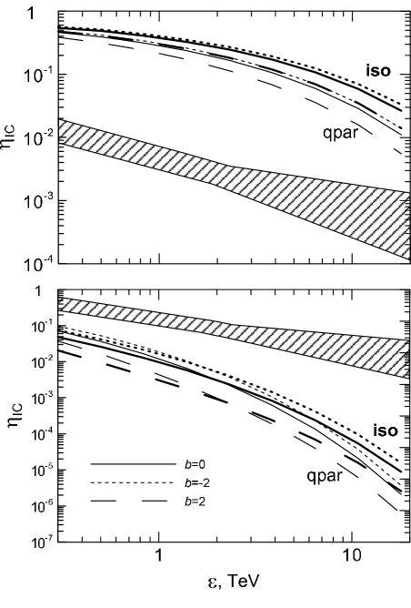
Figure 13: Modification factor $\eta_{\mathrm{ic}}$. Lines are the same as on Fig. 11. Experimental modification factor for SN 1006 are shown for comparison. It is obtained from the HESS data (Acero et al., 2010) with the use of Eq. (11) and MF strength $B_{\mathrm{o}}=3{\,\rm\mu G}$ (upper panel) and $B_{\mathrm{o}}=30{\,\rm\mu G}$ (lower panel).

The contribution from electrons with energies around $E_{\mathrm{max}}$ may be important for TeV $\gamma$-photons. The full expression for IC process is

$$F_{\mathrm{ic}}(\varepsilon)=C_{\mathrm{ic}}\zeta_{\mathrm{ic}}(\varepsilon;b,\Theta_{\mathrm{K}},\epsilon_{\mathrm{f\|}},E_{\mathrm{max\|}})K_{\mathrm{s\|}}R^{3}d^{-2}$$ (45)

where

$$C_{\mathrm{ic}}=\frac{3\sigma_{\mathrm{T}}kT_{\mathrm{CMB}}(m_{\mathrm{e}}c^{2})^{3-s}}{2h^{3}c^{2}},$$ (46)

$$\begin{array}[]{l}\zeta_{\mathrm{ic}}({\varepsilon};b,\Theta_{\mathrm{K}},\epsilon_{\mathrm{f\|}},E_{\mathrm{max\|}})=\displaystyle\int\limits_{0}^{2\pi}\!d\varphi\!\int\limits_{0}^{\pi}\!\!d\theta\sin\theta f_{\mathrm{K}}\!\int\limits_{0}^{1}\!\!d\bar{a}\bar{r}^{2}\bar{r}_{\mathrm{\bar{a}}}\bar{K}\!\\ \\ \quad\times\displaystyle\int\limits_{\gamma_{\mathrm{min}}(\varepsilon)}^{\infty}\!d\gamma\gamma^{-2-s}{\cal E}_{\mathrm{rad}}^{s-2}\exp\left(-\frac{\gamma}{\gamma_{\mathrm{max\|}}{\cal E}_{\mathrm{ad}}{\cal E}_{\mathrm{rad}}f_{\mathrm{E}}}\right){\cal I}(\varepsilon,E),\end{array}\!\!\!\!\!$$ (47)

where $\gamma$ is the electron Lorentz factor, ${\cal I}$ is an integral appearing in the theory of inverse-Compton process (e.g., Petruk, 2008); it accounts for the KN decline where nesessary.

In case $s=2$ and $T_{\mathrm{CMB}}=2.75$, ${\cal A}_{\mathrm{T}}=0.710$ and $C_{\mathrm{T}}=1.304\times 10^{-14}{\,\rm cgs}$, $C_{\mathrm{ic}}=1.186\times 10^{12}{\,\rm cgs}$.

In the limit $E\ll E_{\mathrm{max}}$ and $E\ll\epsilon_{\mathrm{f}}E_{\mathrm{max}}$, one has ${\cal E}_{\mathrm{rad}}=1$ and ${\cal I}\propto\varepsilon$, $E_{\mathrm{min}}\propto\varepsilon^{1/2}$ (Petruk, 2008) and (45) transforms to (41). Therefore

$$\zeta_{\mathrm{ic}}({\varepsilon})=c_{\mathrm{o}}{\varepsilon}^{-(s-1)/2}\zeta_{\mathrm{T}}$$ (48)

in this limit; $c_{\mathrm{o}}=C_{\mathrm{T}}/C_{\mathrm{ic}}$.

Let us introduce the modification factor for IC spectrum:

$$\eta_{\mathrm{ic}}(\varepsilon,\epsilon_{\mathrm{f\|}},E_{\mathrm{max\|}})=\frac{\zeta_{\mathrm{ic}}({\varepsilon},\epsilon_{\mathrm{f\|}},E_{\mathrm{max\|}}){\varepsilon}^{(s-1)/2}}{c_{\mathrm{o}}\zeta_{\mathrm{T}}}.$$ (49)

It is also defined to be $\eta_{\mathrm{ic}}\leq 1$ and ensure $\eta_{\mathrm{ic}}\rightarrow 1$ well below TeV energies. However, it is not so universal as for the synchrotron emission, Eq. (39): it does not scaled with the frequency and it depends on the absolute value of $E_{\mathrm{max}}$. The expression for the broadband IC spectrum is

$$F_{\mathrm{ic}}(\varepsilon)=C_{\mathrm{T}}\varepsilon^{-(s-1)/2}\zeta_{\mathrm{T}}(b,\Theta_{\mathrm{K}})\eta_{\mathrm{ic}}(\varepsilon,\epsilon_{\mathrm{f\|}},E_{\mathrm{max\|}})K_{\mathrm{s\|}}R^{3}d^{-2}.$$ (50)

The parameter $\zeta_{\mathrm{T}}$ behaves like $\zeta$ (Fig. 12): it mostly depends on $\Theta_{\mathrm{K}}$ for quasiparallel injection and on $b$ for isotropic injection. However, the role of $\zeta_{\mathrm{T}}$ is less important for normalization of IC spectrum because it varies in about 4 times over the parameter space.

The modification factor of the IC specrum $\eta_{\mathrm{ic}}$ is shown on Fig. 13, in comparison with the observational data for SN 1006. It depends on $\epsilon_{\mathrm{f\|}}$, $b$, $\Theta_{\mathrm{K}}$, $s$ and $E_{\mathrm{max}}$ as well as on the function $f_{\mathrm{E}}(\Theta_{\mathrm{o}})$.

References

- Acero et al. (2010) Acero F., et al. A&A 516, id.A62
- Aharonian & Atoyan (1999) Aharonian F. & Atoyan A., 1999, A&A, 351, 330
- Aharonian et al. (2006) Aharonian F. et al., 2006, A&A 449, 223
- Allen et al. (2008) Allen G. E., Houck J.C., Sturner S. J. 2008, ApJ 683, 773
- Ballet (2005) Ballet J. 2006, Adv. Space Res., 37, 1902
- Bamba et al. (2008) Bamba A., Fukazawa Y., Hiraga J., et al. 2008 PASJ 60, S153
- Berezhko & Völk (2004) Berezhko E. G. & Völk H. J. 2004, A&A 419, L27
- Berezhko & Völk (2006) Berezhko E. G., & Völk H. J. 2006, A&A 451, 981
- Berezhko et al. (2003) Berezhko E. G., Ksenofontov L. T., Völk H. J. 2003, A&A 412, L11
- Berezhko et al. (2009) Berezhko E. G., Ksenofontov L. T., Völk H. J. 2009, A&A, 505, 169
- Cassam-Chenaï et al. (2008) Cassam-Chenaï, G., Hughes, J. P., Reynoso, E. M., Badenes, C., & Moffett, D. 2008, ApJ, 680, 1180
- Ellison et al. (1995) Ellison D. C., Baring M. G., Jones F. C., 1995 ApJ, 453, 873
- Ellison et al. (2000) Ellison D. C., Berezhko E. G., Baring M. G. 2000, ApJ, 540, 292
- Hnatyk & Petruk (1999) Hnatyk B. & Petruk O. 1999, A&A, 344, 295
- Katsuda et al. (2010) Katsuda, S., Robert Petre, R., Mori, K. et al. 2010, ApJ, 723, 383
- Ksenofontov et al. (2005) Ksenofontov L. T., Berezhko E. G., Voelk H. J. 2005, A&A 443, 973
- Long et al. (2003) Long K. S., Reynolds S. P., Raymond J. C., et al. 2003, ApJ, 586, 1162
- Miceli et al. (2009) Miceli M., Bocchino F., Iakubovskyi D., Orlando S., Telezhinsky I., Kirsch M. G. F., Petruk O., Dubner G., Castelletti G., 2009, A&A, 501, 239
- Milne (1971) Milne D. K. 1971, Australian J. Phys., 24, 757
- Orlando et al. (2007) Orlando S., Bocchino F., Reale F., Peres G., Petruk O. 2007, A&A, 470, 927
- Orlando et al. (2010) Orlando S., Petruk O., Bocchino F., Miceli M., 2010, A&A in press (arXiv:1011.1847)
- Petruk (2001) Petruk O., 2001, A&A, 371, 267
- Petruk (2006) Petruk O., 2006, A&A, 460, 375
- Petruk (2008) Petruk O., 2008, A&A, 499, 643
- Petruk & Beshley (2007) Petruk O., Beshley V., 2007, KPCB, 23, 16
- Petruk & Beshley (2008) Petruk O., Beshley V., 2008, KPCB, 24, 159
- Petruk et al. (2009a) Petruk O., Beshley V., Bocchino F., & Orlando S., 2009a, MNRAS, 395, 1467
- Petruk et al. (2009b) Petruk O., Bocchino F., Miceli M., Dubner G., Castelletti G., Orlando S., Iakubovskyi D., Telezhinsky I., 2009b, MNRAS, 399, 157
- Petruk et al. (2009c) Petruk O., Dubner G., Castelletti G., Iakubovskyi D., Kirsch M., Miceli M., Orlando S., Telezhinsky I., 2009c, MNRAS, 393, 1034
- Reynolds (1996) Reynolds S. P., 1996, ApJ, 459, L13
- Reynolds (1998) Reynolds S. P., 1998, ApJ, 493, 375
- Rothenflug et al. (2004) Rothenflug R., Ballet J., Dubner G., Giacani E., Decourchelle A., & Ferrando P., 2004, A&A, 425, 121
- Sedov (1959) Sedov L.I., 1959, Similarity and Dimensional Methods in Mechanics (New York, Academic Press).
- Schneiter et al. (2010) Schneiter E. M., Velaźquez P. F., Reynoso E. M., de Colle F. 2010, MNRAS, 408, 430
- Schure et al. (2010) Schure K. M., Achterberg A., Keppens R., Vink J. 2010, MNRAS, 406, 2633
- Völk et al. (2008) Völk H. J., Ksenofontov L. T., Berezhko E. G. 2008, A&A, 490, 515
- Zirakashvili & Aharonian (2007) Zirakashvili V., Aharonian F., 2007, A&A, 465, 695