Dynamical analysis of the exclusive queueing process

Abstract

In a recent study RefAY the stationary state of a parallel-update TASEP with varying system length, which can be regarded as a queueing process with excluded-volume effect (exclusive queueing process, EQP), was obtained. We analyze the dynamical properties of the number of particles $\langle N_{t}\rangle$ and the position of the last particle (the system length) $\langle L_{t}\rangle$, using an analytical method (generating function technique) as well as a phenomenological description based on domain wall dynamics and Monte Carlo simulations. The system exhibits two phases corresponding to linear convergence or divergence of $\langle N_{t}\rangle$ and $\langle L_{t}\rangle$. These phases can both further be subdivided into high-density and maximal-current subphases. The predictions of the domain wall theory are found to be in very good agreement quantitively with results from Monte Carlo simulations in the convergent phase. On the other hand, in the divergent phase, only the prediction for $\langle N_{t}\rangle$ agrees with simulations.

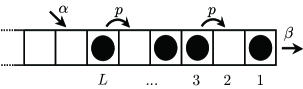
Figure 1: Exclusive queueing process.

I Introduction

Queueing processes have been studied extensively, especially due to their practical relevance RefE ; RefK ; RefS . However, usually the spatial structure of the queues is neglected and the particles in the queues do not interact with each other. On the other hand, the totally asymmetric simple exclusion process (TASEP) which has a spatial structure and excluded-volume effect (hard-core repulsion) is one of the best-studied interacting particle systems RefL . Nowadays the TASEP is a basic model for pedestrian and traffic flows RefCSS ; RefSCN .

Recently a queueing process with the excluded-volume effect, the exclusive queueuing process (EQP), was introduced in RefA and RefY independently, where the model was formulated as continuous-time and discrete-time Markov processes, respectively. This model can be rephrased as the TASEP on a semi-infinite chain with a new boundary condition, see Fig. 1. The left end is interpreted as the end of the queue where new customers arrive. Therefore particles can enter at the left site next to the leftmost occupied site. The (fixed) rightmost site corresponds to the server. Here particles can leave the system after getting service. In the bulk a particle can hop to its right nearest neighbor site, if the target site is empty. After the study RefY , where the bulk hopping rule is deterministic, the model with discrete time and probabilistic bulk hopping was analyzed RefAY .

Earlier works RefA ; RefAY ; RefY focussed on the exact probability distribution, physical quantities in the stationary state, and the conditions under which the EQP converges to the stationary state. In this paper, we study the dynamical properties by considering the number of particles and the system length which is defined as the position of the leftmost particle. We use the same formalism as in RefY ; RefAY , i.e. discrete time and parallel-update scheme. For generic hopping probability $p$, we will introduce a domain wall prediction, checking it by Monte Carlo simulations. In the deterministic hopping case $p=1$, a rigorous analysis is available, by using the generating function technique RefW .

This paper is organized as follows. In Sec. II, we define the model as a discrete-time Markov process, and review its stationary state based on RefAY , which can be generalized to the inhomogeneous injection case, see also App. A. In Sec. III, we introduce a phenomenological argument on how the number of particles $\langle N_{t}\rangle$ and the system length $\langle L_{t}\rangle$ converge or diverge, showing simulation results. In Sec. IV, we derive the asymptotic behaviors of $\langle N_{t}\rangle$ and $\langle L_{t}\rangle$ rigorously for $p=1$, imposing the initial condition that there is no particle on the chain. Section V is devoted to the conclusion of this paper.

II Model

The EQP is defined on a semi-infinite chain where sites are labeled by natural numbers from right to left (Fig. 1). Particles can enter the chain with probability $\alpha$ only at the left site next to the leftmost occupied site. A particle hops to its right nearest neighbor site with probability $p$, if it is empty, and exits at the right end of the chain with probability $\beta$. If there is no particle on the chain, a particle enters at site 1 with probability $\alpha$. These transitions occur simultaneously within one time step, i.e. we apply the fully-parallel-update scheme.

We formulate the EQP as a discrete-time Markov process on the state space

$$S=\{\emptyset,1,10,11,100,101,110,111,1000,\dots\}$$ (1)

where 0 and 1 correspond to unoccupied and occupied sites, respectively. In particular, $\emptyset$ denotes the state in which there is no particle on the chain. To simplify the notation we do not write the infinite number of 0’s located left to the leftmost 1.

Let us review the matrix product stationary state RefAY of the model, which is a simple extension of that for systems with a fixed system length RefBE . When

$$\begin{cases}\alpha\leq\alpha_{c}=\frac{1-\sqrt{1-p}}{2}&\text{for }\beta>1-\sqrt{1-p},\\ \alpha<\alpha_{c}=\frac{\beta(p-\beta)}{p-\beta^{2}}&\text{for }\beta\leq 1-\sqrt{1-p},\end{cases}$$ (2)

the stationary state can be expressed as

$$P(\emptyset)= \frac{1}{Z}\,,$$ (3)

$$P(1\tau_{L-1}\dots\tau_{1})= \frac{1}{Z}\left(\frac{\alpha}{p(1-\alpha)}\right)^{L}\langle W|DX_{\tau_{L-1}}\cdots X_{\tau_{1}}|V\rangle\,.$$ (4)

$X_{1}=D$ and $X_{0}=E$ are matrices, $\langle W|$ is a row vector and $|V\rangle$ is a column vector satisfying the algebraic relations

$$\begin{split}EDEE=&(1-p)EDE+EEE+pEE,\\ EDED=&EDD+EED+pED,\\ DDEE=&(1-p)DDE+(1-p)DEE\\ &\ +p(1-p)DE,\\ DDED=&DDD+(1-p)DED+pDD,\\ DDE|V\rangle=&(1-\beta)DD|V\rangle+(1-p)DE|V\rangle\\ &\ +p(1-\beta)D|V\rangle,\\ EDE|V\rangle=&(1-\beta)ED|V\rangle+EE|V\rangle+pE|V\rangle,\\ \langle W|DEE=&(1-p)\langle W|DE,\\ \langle W|DED=&\langle W|DD+p\langle W|D,\\ DD|V\rangle=&\frac{p(1-\beta)}{\beta}D|V\rangle,\ ED|V\rangle=\frac{p}{\beta}E|V\rangle,\\ \langle W|EE=&0,\ \langle W|ED=p\langle W|D,\ \langle W|D|V\rangle=\frac{p}{\beta}.\end{split}$$ (5)

These relations are closely related to those for the stationary state of the parallel-update TASEP with ordinary open boundary condition RefERS . The normalization constant is expressed as

$$Z = 1+\sum_{L\geq 1}\left(\frac{\alpha}{p(1-\alpha)}\right)^{L}\langle W|D(D+E)^{L-1}|V\rangle$$ (6)

$$= \frac{2(1-\alpha)\beta}{R-p+2(1-\alpha)\beta}$$ (7)

with $R=\sqrt{p(p-4\alpha(1-\alpha))}$. The average number of particles $\langle N\rangle$ and the average system length (the position of the leftmost particle) $\langle L\rangle$ are calculated as

$$\langle N\rangle= \frac{\alpha(1-\alpha)(p-2\alpha p+R)}{R(R-p+2(1-\alpha)\beta)},$$ (8)

$$\langle L\rangle= \frac{\alpha p(R-p+2(1-\alpha))}{R(R-p+2(1-\alpha)\beta)}$$ (9)

in the stationary state. Note that $\langle N\rangle$ and $\langle L\rangle$ diverge on the critical line $\alpha=\frac{1}{2}(1-\sqrt{1-p})$, $\beta>1-\sqrt{1-p}$, where the stationary state exists.

A generalization of the model, where the entry probability depends on the system length, also has a matrix product stationary state, see App. A.

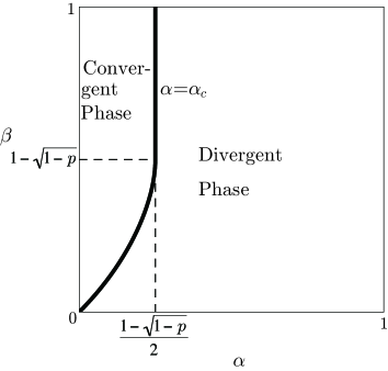
Figure 2: Phase diagram for the EQP. The parameter space is divided into two regions with and without the stationary state.

III Domain wall picture and Monte Carlo simulations

In this section, we discuss the time evolution of the average number of particles $\langle N_{t}\rangle$ and the average system length $\langle L_{t}\rangle$ corresponding to the position of the leftmost particle.

In the ordinary open boundary case, where the length of the system is fixed, a domain wall moves rightward or leftward, or exhibits a random walk depending on the boundary parameters RefKSKS . In the same way, we will discuss how the system length $\langle L_{t}\rangle$ moves. We also observe how the average number of particles $\langle N_{t}\rangle$ changes as well. The continuity equation

$$\langle N_{t+1}\rangle-\langle N_{t}\rangle =J_{t}^{\rm in}-J_{t}^{\rm out}.$$ (10)

holds, where $J_{t}^{\rm in}$ and $J_{t}^{\rm out}$ are the flows of particles entering and leaving the system, respectively. The inflow $J_{t}^{\rm in}$ is always $\alpha$, which is due to the fact that the site where particles enter is by definition never blocked. In other words, our model is not a call-loss system. Under the assumption that the outflow $J^{\rm out}_{t}$ is independent of $t$, we have $\langle N_{t}\rangle=(\alpha-J^{\rm out})t+\langle N_{0}\rangle$. In fact our simulations show that both $\langle N_{t}\rangle$ and $\langle L_{t}\rangle$ decrease or increase linearly in time $t$ according to $\alpha<\alpha_{c}$ or $\alpha>\alpha_{c}$, respectively.

III.1 Convergent Phase

When $\alpha<\alpha_{c}$, the system converges to the stationary state (3), (4). We impose the initial condition that particles are distributed uniformly with density

$$\rho= \begin{cases}\frac{1}{2}&\text{for }\beta>1-\sqrt{1-p},\\ \frac{p-\beta}{p-\beta^{2}}&\text{for }\beta\leq 1-\sqrt{1-p}.\end{cases}$$ (11)

As in Fig. 3, $\langle N_{t}\rangle$ and $\langle L_{t}\rangle$ decrease linearly in time as

$$\langle N_{t}\rangle\sim(\alpha-{J^{\rm out}})t+\langle N_{0}\rangle,$$ (12)

$$\langle L_{t}\rangle\sim\frac{\alpha-{J^{\rm out}}}{\rho}t+\langle L_{0}\rangle,$$ (13)

with

$$\begin{split}J^{\rm out}&=\frac{1-\sqrt{1-4p\rho(1-\rho)}}{2}\\ &=\begin{cases}\frac{1-\sqrt{1-p}}{2}&\text{for }\beta>1-\sqrt{1-p},\\ \frac{\beta(p-\beta)}{p-\beta^{2}}&\text{for }\beta\leq 1-\sqrt{1-p}.\end{cases}\end{split}$$ (14)

Since $J^{\rm out}=\alpha_{c}$, we have $\alpha-J^{\rm out}<0$ which means that the domain wall moves rightward.

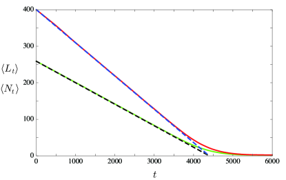
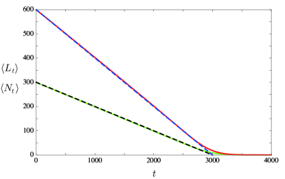
Figure 3: Dynamics in the HD-C (top) and MC-C (bottom) phases. The parameter values are chosen as $(\alpha,\beta,p)=(0.2,0.4,0.84)$ and $(0.2,0.8,0.84)$, and the initial conditions as $(\langle N_{0}\rangle,\langle L_{0}\rangle)=(400\rho,400)$ and $(600\rho,600)$ (with $\rho$ defined by (11)), respectively. The green and red lines are data for $\langle N_{t}\rangle$ and $\langle L_{t}\rangle$ obtained from Monte Carlo simulations, where 5000 samples are averaged. The black and blue lines correspond to the predictions of the domain wall theory. Note that the asymptotic values are small but non-zero (see Eqs. (8) and (9)): $\mathbf{(}\langle N_{\infty}\rangle,\langle L_{\infty}\rangle)=(1.70,2.28)$ and $\mathbf{(}0.42,0.56)$, respectively.

According to the forms for $J^{\rm out}$ and $\rho$, we call the phases

$$\text{MC-C:}\quad\alpha<\frac{1-\sqrt{1-p}}{2}\quad\text{and}\quad\beta>1-\sqrt{1-p},$$ (15)

$$\text{HD-C:}\quad\alpha<\frac{\beta(p-\beta)}{p-\beta^{2}}\quad\text{and}\quad\beta\leq 1-\sqrt{1-p},$$ (16)

maximal-current-convergent (MC-C) and high-density-convergent (HD-C) phases, respectively, see Fig. 4.

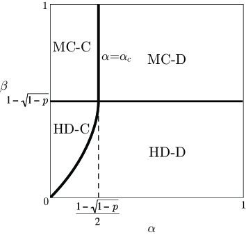
Figure 4: Subphases of the EQP.

It should be noted that the outflow is given by Eqn. (14) only while $0\leq t\lesssim\frac{\langle L_{0}\rangle}{\alpha-J^{\rm out}}$. As $t\to\infty$, the outflow approaches $\alpha$, assuring that $\langle N_{t}\rangle$ approaches the stationary value (8).

Figure 5 shows density profiles in the HD-C and MC-C phases. We can observe that the bulk density keeps its initial value (11).

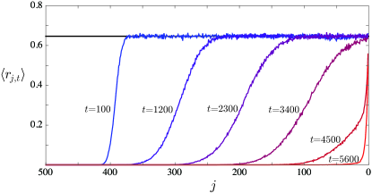
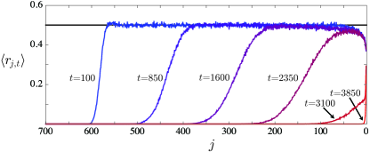
Figure 5: Density profiles ($\langle r_{j,t}\rangle$ of the $j$th site at time $t$) in the HD-C (top) and MC-C (bottom) phases. The parameters $(\alpha,\beta,p)$ and the initial conditions $(\langle N_{0}\rangle,\langle L_{0}\rangle)$ are set to the same values as in Fig. 3. The colored snapshots are obtained by averaging 5000 samples of Monte Carlo simulations. The black lines represent the predicted densities $\rho$ according to Eqn. (11).

III.2 Divergent Phase

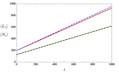
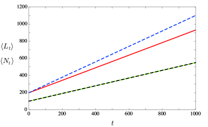
Figure 6: Dynamics in the HD-D (top) and MC-D (bottom) phases. The parameter values are chosen as $(\alpha,\beta,p)=(0.75,0.4,0.84)$ and $(0.75,0.8,0.84)$, respectively, and the initial conditions as $(\langle N_{0}\rangle,\langle L_{0}\rangle)=(200\rho,200)$ (with $\rho$ defined by (11)). The green and red lines are data for $\langle N_{t}\rangle$ and $\langle L_{t}\rangle$ obtained from Monte Carlo simulations, where 1000 samples are averaged. The black and blue lines correspond to the predictions of the domain wall theory.

When $\alpha>\alpha_{c}$, it is natural to expect that the domain wall moves leftward, and the time evolutions of $\langle N_{t}\rangle$ and $\langle L_{t}\rangle$ are expressed by Eqs. (12) and (13), respectively, with the density (11) and the outflow (14). The simulations imply that this is true for $\langle N_{t}\rangle$ with

$$\langle N_{t}\rangle \sim(\alpha-{J^{\rm out}})t+\langle N_{0}\rangle,$$ (17)

but fails for $\langle L_{t}\rangle$, see Fig. 6. This failure is not unexpected since the predicted velocity $\frac{\alpha-{J^{\rm out}}}{\rho}$ can be greater than 1 whereas the length $\langle L_{t}\rangle$ can not be larger than $t+\langle L_{0}\rangle$ by the definition of the model. However, the simulation results (see Fig. 6) indicate that

$$\langle L_{t}\rangle \sim Vt+\langle L_{0}\rangle,$$ (18)

so that the prediction is qualitatively correct. The velocity $V$ satisfies

$$V \to 0\quad(\alpha\to\alpha_{c}),$$ (19)

$$V =1\quad(\alpha=1).$$ (20)

and we have exactly $\langle L_{t}\rangle=t+\langle L_{0}\rangle$ when $\alpha=1$. Moreover, when $p=1$, we will show in the next section that

$$V=\alpha-\beta+\alpha\beta=\frac{\alpha-\frac{\beta}{1+\beta}}{\frac{1}{1+\beta}}=\frac{\alpha-J^{\rm out}}{\rho}.$$ (21)

Equations (17) and (18) can be regarded as the asymptotic behaviors

$$\langle N_{t}\rangle =(\alpha-{J^{\rm out}})t+o(t),$$ (22)

$$\langle L_{t}\rangle =Vt+o(t).$$ (23)

In the same way as in the convergent phase, we call the subphases

$$\text{MC-D:}\quad\alpha>\frac{1-\sqrt{1-p}}{2}\quad\text{and}\quad\beta>1-\sqrt{1-p},$$ (24)

$$\text{HD-D:}\quad\alpha>\frac{\beta(p-\beta)}{p-\beta^{2}}\qquad\text{and}\qquad\beta\leq 1-\sqrt{1-p},$$ (25)

maximal-current-divergent (MC-D) and high-density-divergent (HD-D) phases, respectively. Note that the densities in the MC-D and HD-D phases are higher than (or equal to) $\frac{1}{2}$ and $\frac{p-\beta}{p-\beta^{2}}$, respectively.

It is difficult to predict how $\langle N_{t}\rangle$ or $\langle L_{t}\rangle$ behaves just on the critical line $\alpha=\alpha_{c}$. For $p=1$, however, we will find in the next section diffusive behavior on the critical line as

$$\langle N_{t}\rangle = D_{N}\sqrt{t}+o(\sqrt{t}),$$ (26)

$$\langle L_{t}\rangle = D_{L}\sqrt{t}+o(\sqrt{t})$$ (27)

with constants $D_{N}$ and $D_{L}$.

IV Asymptotic behaviors for $p=1$

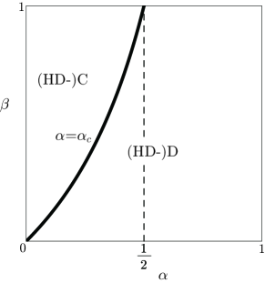
Figure 7: Phase diagram for $p=1$.

In this section we investigate the asymptotic behaviors of $\langle N_{t}\rangle$ and $\langle L_{t}\rangle$ rigorously for $p=1$. Thanks to the deterministic particle hopping we can obtain the generating functions of $\langle N_{t}\rangle$ and $\langle L_{t}\rangle$. For simplicity, we impose the initial condition $\emptyset$ (there is no particle in the system at time $t=0$), and reset the state space as

$$\begin{split}\widetilde{S}&:=\{\emptyset,1,10,11,101,110,111,1010,1011,\dots\}\\ &=\left\{\tau\in S|\tau\ \text{does not contain sequence }00\right\}.\end{split}$$ (28)

Note that, for $p=1$, the sequence 00 never appears if the system starts from the initial condition $\emptyset$. In this case, the MC-D and MC-C phases vanish from the phase diagram, see Fig. 7.

We first consider the number of particles, borrowing the classification from RefY as

$$\begin{split}P_{t}^{A}(N)=&{\rm Prob}\left[\begin{array}[]{l}\text{\# of particles is $N$ at time $t$}\\ \wedge\text{ site 1 is occupied at time $t$}\end{array}\right],\end{split}$$ (29)

$$\begin{split}P_{t}^{B}(N)=&{\rm Prob}\left[\begin{array}[]{l}\text{\# of particles is $N$ at time $t$}\\ \wedge\text{ site 1 is empty at time $t$}\end{array}\right]\end{split}$$ (30)

for $N\in\mathbb{Z}_{\geq 0}$ with $P_{t}^{A}(0)\equiv 0$. These probabilities are governed by the following master equation, which was found in RefY :

$$\begin{split}P_{t+1}^{A}(1)=&(1-\alpha)(1-\beta)P_{t}^{A}(1)+\alpha P_{t}^{B}(0)\\ &\quad\quad\quad\quad\quad+(1-\alpha)P_{t}^{B}(1),\end{split}$$ (31)

$$\begin{split}P_{t+1}^{A}(N)=&\alpha(1-\beta)P_{t}^{A}(N-1)+\alpha P_{t}^{B}(N-1)\\ &\!\!\!\!\!\!\!\!\!+(1-\alpha)(1-\beta)P_{t}^{A}(N)+(1-\alpha)P_{t}^{B}(N),\end{split}$$ (32)

$$P_{t+1}^{B}(0)= (1-\alpha)P_{t}^{B}(0)+(1-\alpha)\beta P_{t}^{A}(1),$$ (33)

$$P_{t+1}^{B}(N)= \alpha\beta P_{t}^{A}(N)+(1-\alpha)\beta P_{t}^{A}(N+1).$$ (34)

This simplification is due to the deterministic hopping $p=1$. We choose the initial condition such that

$$P^{B}_{0}(0)=1,\quad P^{A}_{0}(N)=P^{B}_{0}(N)=0\quad(N\in\mathbb{N}).$$ (35)

We will check that the average number of particles $\langle N_{t}\rangle$ converges to the stationary value (8) when $\alpha<\frac{\beta}{1+\beta}$, and show that $\langle N_{t}\rangle$ behaves as Eqn. (22) when $\alpha>\frac{\beta}{1+\beta}$. We will also show that $\langle N_{t}\rangle$ exhibits diffusive behavior on the critical line $\alpha=\frac{\beta}{1+\beta}$.

We define the generating functions of $P^{A}_{t}(N)$ and $P^{B}_{t}(N)$ as

$$G^{A}_{z}(N) = \sum_{t\geq 0}P_{t}^{A}(N)z^{t},$$ (36)

$$G^{B}_{z}(N) = \sum_{t\geq 0}P_{t}^{B}(N)z^{t},$$ (37)

for $|z|<1$. Noting the initial condition (35), we find

$$\begin{split}&G_{z}^{A}(1)=(1-\alpha)(1-\beta)zG_{z}^{A}(1)+\alpha zG_{z}^{B}(0)\\ &\quad\quad\quad\quad\quad+(1-\alpha)zG_{z}^{B}(1),\end{split}$$ (38)

$$\begin{split}&G_{z}^{A}(N)=\alpha(1-\beta)zG_{z}^{A}(N-1)+\alpha zG_{z}^{B}(N-1)\\ &\quad+(1-\alpha)(1-\beta)zG_{z}^{A}(N)+(1-\alpha)zG_{z}^{B}(N),\end{split}$$ (39)

$$G_{z}^{B}(0)-1=(1-\alpha)zG_{z}^{B}(0)+(1-\alpha)\beta zG_{z}^{A}(1),$$ (40)

$$G_{z}^{B}(N)=\alpha\beta zG_{z}^{A}(N)+(1-\alpha)\beta zG_{z}^{A}(N+1).$$ (41)

From Eqn. (40), we have

$$G_{z}^{B}(0) =\frac{1+(1-\alpha)\beta zG_{z}^{A}(1)}{1-(1-\alpha)z}.$$ (42)

Inserting this and Eqn. (41) into Eqs. (LABEL:GA1) and (LABEL:GAN), we get a recurrence formula for $G_{z}^{A}(N)$ as

$$G_{z}^{A}(2)=-\frac{\alpha}{(1-\alpha)^{2}\beta(1-(1-\alpha)z)z}+\frac{1-(1-\alpha)(2-\beta)z+(1-\alpha)(1-\alpha-\beta-\alpha\beta)z^{2}+(1-\alpha)^{2}\alpha\beta z^{3}}{(1-\alpha)^{2}\beta(1-(1-\alpha)z)z^{2}}G_{z}^{A}(1)$$ (43)

$$\begin{split}&G_{z}^{A}(N+1)=-\frac{1-(1-\alpha)(1-\beta)z-2(1-\alpha)\alpha\beta z^{2}}{(1-\alpha)^{2}\beta z^{2}}G_{z}^{A}(N)+\frac{\alpha(1-\beta)+\alpha^{2}\beta z}{(1-\alpha)^{2}\beta z}G_{z}^{A}(N-1)\\ &\quad\quad\quad\quad\ \Big{(}=:xG_{z}^{A}(N)+yG_{z}^{A}(N-1)\Big{)}\quad\quad(N\in\mathbb{Z}_{\geq 2}).\end{split}$$ (44)

The recurrence formula (LABEL:recursion) has the following solution:

$$\begin{split}G_{z}^{A}(N)=&\frac{\lambda_{+}^{N-1}}{\lambda_{+}-\lambda_{-}}\left(G_{z}^{A}(2)-\lambda_{-}G_{z}^{A}(1)\right)\\ &-\frac{\lambda_{-}^{N-1}}{\lambda_{+}-\lambda_{-}}\left(G_{z}^{A}(2)-\lambda_{+}G_{z}^{A}(1)\right),\end{split}$$ (45)

where

$$\lambda_{\pm}=\frac{1-(1-\alpha)(1-\beta)z-2(1-\alpha)\alpha\beta z^{2}\pm r}{2(1-\alpha)^{2}\beta z^{2}}$$ (46)

with

$$r=\sqrt{(1-(1-\alpha)(1-\beta)z)^{2}-4(1-\alpha)\alpha\beta z^{2}}$$ (47)

are solutions to $\lambda^{2}=x\lambda+y$ with $x$ and $y$ as defined in Eqn. (LABEL:recursion). Restricting the “initial condition” $G^{A}_{z}(1)$ and $G^{A}_{z}(2)$ such that

$$\left|G^{A}_{z}(N)\right|<\sum_{t\geq 0}|z|^{t}=\frac{1}{1-|z|},$$ (48)

we have

$$G_{z}^{A}(2)-\lambda_{-}G_{z}^{A}(1)=0.$$ (49)

(Note that $0<|\lambda_{-}|<1<|\lambda_{+}|$.) From this constraint and the relation (43) $G^{A}_{Z}(1)$ is determined, and we find

$$G_{z}^{A}(N) =\lambda_{-}^{N-1}G_{z}^{A}(1)=\lambda_{-}^{N-1}\frac{-1+(1-\alpha)(2-\beta)z-(1-\alpha)(1-\alpha-\beta-\alpha\beta)z^{2}+(1-(1-\alpha)z)r}{2(1-\alpha)^{2}\beta^{2}(1-z)z^{2}}\quad(N\in\mathbb{N}),$$ (50)

$$G_{z}^{B}(0) =\frac{-1+r+(1-\alpha)(1+\beta)z}{2(1-\alpha)\beta z(1-z)},\qquad G_{z}^{B}(N)=\left(\alpha+(1-\alpha)\lambda_{-}\right)\beta z\lambda_{-}^{N-1}G_{z}^{A}(1)\quad(N\in\mathbb{N}).$$ (51)

Then we obtain the generating function $G_{z}(N)$ of the probability that the number of particles is $N$ as

$$G_{z}(0)= ~{}G_{z}^{B}(0),\quad G_{z}(N)=G_{z}^{A}(N)+G_{z}^{B}(N)=g(z)\lambda_{-}^{N},$$ (52)

$$g(z)= \,\frac{\beta-1+\left(1-\alpha-\beta+\beta^{2}-\alpha\beta^{2}\right)z+(1-\alpha)(1-\beta)\beta z^{2}+r(1-(1-z)\beta)}{2\beta(1-\alpha)(1-(1-z\alpha)\beta)(1-z)z}\quad(N\in\mathbb{N}).$$ (53)

We also introduce the generating function ${\mathcal{G}}_{z\zeta}$ of the generating function $G_{z}(N)$ as

$$\begin{split}{\mathcal{G}}_{z\zeta}&=\sum_{N\geq 0}G_{N}(z)\zeta^{N}=G_{0}(z)+\sum_{N\geq 1}g(z)(\lambda_{-}\zeta)^{N}\\ &=G_{0}(z)+g(z)\frac{\lambda_{-}\zeta}{1-\lambda_{-}\zeta},\end{split}$$ (54)

and $K_{z}$ of the average number of particles as

$$\begin{split}K_{z}&=\sum_{t\geq 0}z^{t}\langle N_{t}\rangle=\sum_{t\geq 0}z^{t}\sum_{N\geq 0}N\left(P^{A}_{t}(N)+P^{B}_{t}(N)\right)\\ &=\left.\frac{\partial}{\partial\zeta}{\mathcal{G}}_{z\zeta}\right|_{\zeta=1}=\frac{z(2\alpha-1+z(1-\alpha)(1-\beta)+r)}{2(1-z)^{2}(1+z\beta)}.\end{split}$$ (55)

The asymptotic behavior of $\langle N_{t}\rangle$ is determined by the degree of the singularity $z=1$ of $K_{z}$ RefW . When $\alpha<\frac{\beta}{1+\beta}$, we find

$$(1-z)K_{z}\Big{|}_{z\to 1}=\frac{\alpha(1-\alpha)}{\beta-\alpha-\alpha\beta},$$ (56)

and $\langle N_{t}\rangle$ converges as

$$\langle N_{t}\rangle\to\frac{\alpha(1-\alpha)}{\beta-\alpha-\alpha\beta}\quad\quad(t\to\infty).$$ (57)

Of course this limit value agrees with the stationary value (8) with $p=1$. When $\alpha>\frac{\beta}{1+\beta}$, we find

$$(1-z)^{2}K_{z}\Big{|}_{z\to 1}=\alpha-\frac{\beta}{1+\beta},$$ (58)

and $\langle N_{t}\rangle$ behaves as

$$\langle N_{t}\rangle =\left(\alpha-\frac{\beta}{1+\beta}\right)t+o(t)$$ (59)

$$=(\alpha-J^{\rm out})t+o(t)\quad\quad(t\to\infty).$$ (60)

When $\alpha=\frac{\beta}{1+\beta}$, we find

$$(1-z)^{\frac{3}{2}}K_{z}\Big{|}_{z\to 1}=\sqrt{\frac{\beta}{(1+\beta)^{3}}},$$ (61)

and $\langle N_{t}\rangle$ behaves as

$$\langle N_{t}\rangle=2\sqrt{\frac{\beta t}{\pi(1+\beta)^{3}}}+o\left(\sqrt{t}\right)\quad\quad(t\to\infty).$$ (62)

Now we turn to the behavior of the length of the system (the position of the leftmost particle). Let $Q_{t}(L)$ be the probability that the system length is $L$ at time $t$. The probability $Q_{t}(L)$ is governed by

$$Q_{t+1}(0) = (1-\alpha)Q_{t}(0)+\beta(1-\alpha)Q_{t}(1),$$ (63)

$$Q_{t+1}(L) = \alpha Q_{t}(L-1)+(1-\alpha)(1-\beta)Q_{t}(L)$$ (64)

$$+(1-\alpha)\beta Q_{t}(L+1)$$

for $L\in\mathbb{N}$. The first equation means that, if there is no particle at time $t+1$, there is no particle at time $t$ and no particle enters (with probability $1-\alpha$), or there is only one particle on the rightmost site at time $t$ which leaves the system and no particle enters (with probability $(1-\alpha)\beta$). The second equation is derived in App. B.

In the same way as for the number of particles, we define the generating function $M_{z}(L)=\sum_{t\geq 0}z^{t}Q_{t}(L)\ (|z|<1)$. Noting the initial condition $Q_{0}(0)=1$ and $Q_{0}(L)=0\ (L\in\mathbb{N})$, we find

$$\begin{split}M_{z}(1)=&\,\frac{1-(1-\alpha)z}{(1-\alpha)\beta z}M_{z}(0)-\frac{1}{(1-\alpha)\beta z},\end{split}$$ (65)

$$\begin{split}M_{z}(L+1)=&\,\frac{1-(1-\alpha)(1-\beta)z}{(1-\alpha)\beta z}M_{z}(L)\\ &\,-\frac{\alpha}{(1-\alpha)\beta}M_{z}(L-1)\\ \big{(}=:&\,XM_{z}(L)+YM_{z}(L-1)\big{)}.\end{split}$$ (66)

The solution to the recurrence formula (66) is

$$\begin{split}M_{z}(L)=&\frac{\Lambda_{+}^{L}}{\Lambda_{+}-\Lambda_{-}}\left(M_{z}(1)-\Lambda_{-}M_{z}(0)\right)\\ &-\frac{\Lambda_{-}^{L}}{\Lambda_{+}-\Lambda_{-}}\left(M_{z}(1)-\Lambda_{+}M_{z}(0)\right),\end{split}$$ (67)

where $\Lambda_{\pm}=\frac{1-(1-\alpha)(1-\beta)z\pm r}{2(1-\alpha)\beta z}$ are the solutions to $\Lambda^{2}=X\Lambda+Y$ with $X$ and $Y$ as defined in Eqn. (66). Due to the condition $\left|M_{z}(L)\right|<\frac{1}{1-|z|}$, the “initial condition” must be restricted as

$$M_{z}(1)-\Lambda_{-}M_{z}(0)=0.$$ (68)

(Note that $0<|\Lambda_{-}|<1<|\Lambda_{+}|$.) Thus we find

$$M_{z}(L)=M_{z}(0)\Lambda_{-}^{L}=\frac{2}{1-(1-\alpha)(1+\beta)z+r}\Lambda_{-}^{L}.$$ (69)

The generating function of the generating function is calculated as

$${\mathcal{M}}_{z\xi}=\sum_{L\geq 0}\xi^{L}M_{z}(L)=\frac{M_{z}(0)}{1-\xi\Lambda_{-}},$$ (70)

and that of the average system length as

$$\begin{split}S_{z}&=\sum_{t\geq 0}z^{t}\langle L_{t}\rangle=\sum_{t\geq 0}z^{t}\sum_{L\geq 0}LQ_{t}(L)\\ &=\left.\frac{\partial}{\partial\xi}{\mathcal{M}}_{z\xi}\right|_{\xi=1}=\frac{-1+(1+\alpha-\beta+\alpha\beta)z+r}{2(1-z)^{2}}.\end{split}$$ (71)

The asymptotic behavior of $\langle L_{t}\rangle$ is determined by the degree of the singularity $z=1$ of $S_{z}$. When $\alpha<\frac{\beta}{1+\beta}$, we find

$$(1-z)S_{z}\Big{|}_{z\to 1}=\frac{\alpha}{\beta-\alpha-\alpha\beta},$$ (72)

and $\langle L_{t}\rangle$ converges as

$$\langle L_{t}\rangle\to\frac{\alpha}{\beta-\alpha-\alpha\beta}\quad\quad(t\to\infty).$$ (73)

Again this limit value agrees with the stationary value (9) with $p=1$. When $\alpha>\frac{\beta}{1+\beta}$, we find

$$(1-z)^{2}S_{z}\Big{|}_{z\to 1}=\alpha-\beta+\alpha\beta,$$ (74)

and $\langle L_{t}\rangle$ behaves as

$$\langle L_{t}\rangle =\frac{\alpha-\frac{\beta}{1+\beta}}{\frac{1}{1+\beta}}t+o(t)$$ (75)

$$=\frac{\alpha-J^{\rm out}}{\rho}t+o(t)\quad\quad(t\to\infty).$$ (76)

When $\alpha=\frac{\beta}{1+\beta}$, we find

$$(1-z)^{\frac{3}{2}}S_{z}\Big{|}_{z\to 1}=\sqrt{\frac{\beta}{1+\beta}},$$ (77)

and $\langle L_{t}\rangle$ behaves as

$$\langle L_{t}\rangle=2\sqrt{\frac{\beta t}{\pi(1+\beta)}}+o\left(\sqrt{t}\right)\quad\quad(t\to\infty).$$ (78)

V Conclusion

We have investigated the dynamical properties of the EQP, a queueing process with excluded-volume effect. The model can be interpreted as a TASEP with varying length. Using generating function techniques and a phenomenological domain wall theory we have derived analytical predictions for the time-dependence of the number of particles $\langle N_{t}\rangle$ and the average system length $\langle L_{t}\rangle$.

We found that the two phases observed previously can be divided in subphases. The convergent phase, where the system length remains finite, consists of high-density and maximal current subphases. The same is true for the diverging phase, where the system length becomes infinite in the long time limit.

By comparing with Monte Carlo simulations it was found that the predications of the domain wall theory for the dynamical behavior are at least qualitatively correct, i.e. $\langle L_{t}\rangle$ and $\langle N_{t}\rangle$ converge or diverge linearly in time. Moreover they are in good agreement even quantitively in the convergent phase. In the divergent phase, the predicted velocity for $\langle N_{t}\rangle$ appears to be correct whereas deviations from the domain wall theory can be observed for $\langle L_{t}\rangle$.

For $p=1$, we derived exact analytical results for the behaviors of $\langle N_{t}\rangle$ and $\langle L_{t}\rangle$ by using the generating function method. We showed the linearity of their dynamics in the divergent phase as predicted by the domain wall theory. We found diffusive behavior on the critical line as well.

The simple approach presented here does not provide a good expression for the velocity $V$ of the system length ($\langle L_{t}\rangle\sim Vt$) in the divergent phase. Here further analysis of the detailed density profiles in the divergent phase may be helpful. A first step would be the numerical determination of $V$ to get a better understanding of its dependence on the parameters $\alpha,\beta$ and $p$. Another way to settle the problem is extending the exact result to $p<1$ case, which may be difficult but very worthwhile.

Appendix A Stationary State for Inhomogeneous Injection Case

Here we consider the stationary state for a generalized model where the entry probability depends on the system length. A new particle enters the system with probability $\alpha_{L}$ if the leftmost occupied site is $L$, or $\alpha_{0}$ if there is no particle on the chain. The stationary state of this generalized model can be written in the following matrix product form with the same matrices and vectors ($D,E,\langle W|$ and $|V\rangle$):

$$P(\tau_{L}\cdots\tau_{1})=\frac{1}{Z}\frac{\prod_{j=0}^{L-1}\alpha_{j}}{p^{L}\prod_{j=1}^{L}(1-\alpha_{j})}\langle W|X_{\tau_{L}}\cdots X_{\tau_{1}}|V\rangle,$$ (79)

$$Z=1+\sum_{L\geq 1}\frac{\prod_{j=0}^{L-1}\alpha_{j}}{p^{L}\prod_{j=1}^{L}(1-\alpha_{j})}\langle W|D(D+E)^{L-1}|V\rangle.$$ (80)

This can be proved in the same way as in the homogeneous case $\alpha_{L}=\alpha$, see RefAY .

Appendix B Derivation of Eqn. (64)

To derive Eqn. (64), we show

$$\begin{split}&\beta Q_{t}(L)\\ &={\rm Prob}\left[\begin{array}[]{l}\text{the system length is $L$ at time $t$}\\ \wedge\text{ ($L-1$)th site is empty at time $t$}\end{array}\right],\end{split}$$ (81)

$$\begin{split}&(1-\beta)Q_{t}(L)\\ &={\rm Prob}\left[\begin{array}[]{l}\text{the system length is $L$ at time $t$}\\ \wedge\text{ ($L-1$)th site is occupied at time $t$}\end{array}\right],\end{split}$$ (82)

for $L\in\mathbb{N}_{\geq 2}$

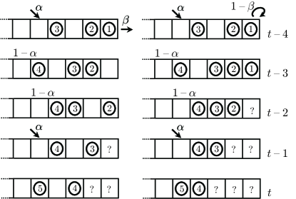
Figure 8: Example for transitions from $1011$ at time $t-4$ to the states in which the system length is 5 and the 4th site is empty (left) or occupied (right) at time $t$.

In the deterministic hopping case $p=1$ with the initial condition $\emptyset$, the sequence 00 (except the infinite number of 0’s left to the leftmost particle) never appears, and holes necessarily “hop” leftward. Thus the first site must be occupied by a particle at time $t-L+1$ if the system length at time $t$ is $L$. The local state (empty or occupied) of the $(L-1)$th site at time $t$ depends only on whether the first particle exits or not at time $t-L+1$. Let the number of particles be $n$ at time $t-L+1$, and label the particles by natural numbers as in Fig. 8. We can show by induction that the $\ell$th particle is on the $\ell$th site at time $t-L+\ell$. Thus we find that $L-n$ new particles should enter the system during $[t-L+1,t-1]$.

We obtain (the summation of) the transition probability from a configuration $S^{(t-L+1)}$ at time $t-L+1$ to the states in which the system length is $L$ and the $(L-1)$th site is empty or occupied at time $t$ is given by

$$\begin{split}&\sum_{S^{(t)},\dots,S^{(t-L+2)}\in\widetilde{S}\atop|S^{(t)}|=L,(S^{(t)})_{L-1}=0}\prod_{t^{\prime}=t-L+1}^{t-1}W(S^{(t^{\prime})}\to S^{(t^{\prime}+1)})\\ &\ =\left(\begin{array}[]{c}L-1\\ L-n\end{array}\right)\alpha^{L-n}(1-\alpha)^{n-1}\beta,\end{split}$$ (83)

$$\begin{split}&\sum_{S^{(t)},\dots,S^{(t-L+2)}\in\widetilde{S}\atop|S^{(t)}|=L,(S^{(t)})_{L-1}=1}\prod_{t^{\prime}=t-L+1}^{t-1}W(S^{(t^{\prime})}\to S^{(t^{\prime}+1)})\\ &\ =\left(\begin{array}[]{c}L-1\\ L-n\end{array}\right)\alpha^{L-n}(1-\alpha)^{n-1}(1-\beta),\end{split}$$ (84)

respectively, where $W(S^{(t^{\prime})}\to S^{(t^{\prime}+1)})$, $|S^{(t^{\prime})}|$ and $(S^{(t^{\prime})})_{j}$ denote the transition probability from $S^{(t^{\prime})}$ to $S^{(t^{\prime}+1)}$, the length of the state $S^{(t^{\prime})}$ and the local state of site $j$. The binomial $\left(\begin{array}[]{c}L-1\\ L-n\end{array}\right)$ gives the number of possibilities for when the new particles enter the system. These equations lead to Eqs. (LABEL:betaQ) and (LABEL:1-betaQ).

If the length is $L$ at time $t+1$, there are the following three possibilities at time $t$:

• the length is $L-1$ and a new particle enters (with probability $\alpha$),

• the length is $L$, the ($L-1$)th site is occupied, and no particle enters (with probability $1-\alpha$),

• the length is $L+1$, the $L$th site is empty, and no particle enters (with probability $1-\alpha$).

Then we achieve Eqn. (64) for $L\in\mathbb{Z}_{\geq 2}$. For $L=1$, the case (ii) is replaced by

• the length is 1, the particle at the rightmost site does not leave, and no particle enters (with probability $(1-\alpha)(1-\beta)$).

References

(1)
C Arita and D Yanagisawa:
J. Stat. Phys. 141, 829 (2010)
(2)
A K Erlang:
Nyt. Tidsskr. Mat. Ser. B 20, 33 (1909)
(3)
D G Kendall:
J. Roy. Statist. Soc. Ser. B 13(2), 151 (1951)
(4)
T L Saaty: Elements of Queueing Theory With Applications,
Dover Publ. (1961)
(5)
T M Liggett,
Stochastic Interacting Systems:
Contact, Voter and Exclusion Processes,
Springer, New York (1999)
(6)
D Chowdhury, L Santen and A Schadschneider:
Phys. Rep. 329, 199 (2000)
(7)
A Schadschneider, D Chowdhury and K Nishinari,
Stochastic Transport in Complex Systems: From Molecules to Vehicles,
Elsevier Science, Amsterdam (2010)
(8)
C Arita:
Phys. Rev. E 80, 051119 (2009)
(9)
D Yanagisawa, A Tomoeda, R Jiang and K Nishinari:
JSIAM Lett. 2, 61 (2010)
(10)
R A Blythe and M R Evans:
J. Phys. A: Math. Gen. 40, R333 (2007)
(11)
M R Evans, N Rajewsky and E R Speer,
J. Stat. Phys. 95, 45–96 (1999)
(12)
A B Kolomeisky, G M Schütz, E B Kolomeisky and J P Straley:
J. Phys. A: Math. Gen. 31 6911 (1998)
(13)
H S Wilf, Generatingfunctionology, Academic Press, San Diego
(1994)