High Throughput Software for Powder Diffraction and its Application to Heterogeneous Catalysis
Taha Sochi
A dissertation submitted to
the Department of Crystallography
Birkbeck College London
in fulfillment of the requirements for the degree of
Doctor of Philosophy

Declaration
The work presented in this thesis is the result of my own effort, except where otherwise stated. All sources are acknowledged by explicit reference.

Taha Sochi …………………….

Abstract
In this thesis we investigate high throughput computational methods for processing large quantities of data collected from synchrotron radiation facilities and its application to spectral analysis of powder diffraction data. We also present the main product of this PhD programme, specifically a computer software called ‘EasyDD’ developed by the author as part of this project. This software was created to meet the increasing demand on data processing and analysis capabilities as required by modern detectors which produce huge quantities of data.

The principal objective of EasyDD project was to develop a computer code for visualisation, batch fitting and bulk analysis of large volumes of diffraction data, mainly those obtained from synchrotron radiation sources. Such a tool greatly assists studies on various materials systems and enables far larger detailed data sets to be rapidly interrogated and analysed. Modern detectors coupled with the high intensity X-ray sources available at synchrotron facilities have led to the situation where data sets can be collected in ever shorter time scales and in ever larger numbers. Such large volumes of data sets pose a data processing bottleneck which is set to augment with current and future instrument development. EasyDD has achieved its main objectives and made significant contributions to scientific research. Some of its functionalities have even surpassed the original expectations. More importantly, it can be used as a model for more mature attempts in the future.

EasyDD is currently in use by a number of researchers in a number of academic and research institutions, such as University College London and Rutherford-Appleton Laboratory, to process high-energy diffraction data for various purposes. These include data collected by different techniques such as energy dispersive diffraction (EDD), angle dispersive diffraction (ADD) and Computer Aided Tomography (CAT). EasyDD has already been used in a number of studies such as Lazzari et al [88] and Espinosa-Alonso et al [49]. It is also in use by the High Energy X-Ray Imaging Technology (HEXITEC) project [72] and has been commended by the scientists who work on the development of HEXITEC detectors. The program proved to be efficient and time saving, and hence has met its main objectives in saving valuable resources and enabling rapid data processing and analysis.

The software was also used by the author to process and analyse data sets collected from synchrotron radiation facilities. In this regard, the thesis will present novel scientific research involving the use of EasyDD to handle large diffraction data sets in the study of alumina-supported metal oxide catalyst bodies. These data were collected using Tomographic Energy Dispersive Diffraction Imaging (TEDDI) and Computer Aided Tomography techniques.

Acknowledgements
I would like to thank

• My supervisors Professor Paul Barnes and Dr Simon Jacques for their kindness, help and advice and for offering me a scholarship to study crystallography at Birkbeck College London. Dr Simon Jacques should be accredited for providing some of the ideas of the software developed in the course of this PhD, namely EasyDD.

• The Engineering and Physical Sciences Research Council (EPSRC) for funding this research.

• The Chemistry Department of the University College London and the Crystallography Department of the Birkbeck College London for in-house support.

• The external examiner Professor Mike Glazer from the University of Oxford, and the internal examiner Dr Dewi Lewis from the University College London for their constructive remarks and recommendations which improved the quality of this work.

Nomenclature

$\beta$	peak broadening due to crystallite size
$\theta$	diffraction angle
$2\theta$	scattering angle
$\kappa$	crystallite shape factor
$\lambda$	wavelength
$\sigma$	standard deviation
$\sigma^{2}$	variance
$\tau$	mean size of crystallites
$\chi^{2}$	goodness-of-fit index
$A$	area under peak
$c$	speed of light in vacuum (299 792 458 m.s-1)
$C$	number of constraints
$d$	crystal lattice planar spacing
$E$	energy
$f$	frequency
$F$	Full Width at Half Maximum
$h$	Planck’s constant ($6.6260693\times 10^{-34}$ J.s)
$hkl$	Miller indices
${\rm i}$	imaginary unit ($\sqrt{-1}$)
${I}$	integrated intensity
${I}^{c}$	calculated integrated intensity
${I}^{o}$	observed integrated intensity
$L_{2}$	second norm of residuals
$m$	mixing factor in pseudo-Voigt function
$n$	diffraction order number
$O$	number of observations
$P$	number of parameters
$Q$	quality factor
$r$	radius
$R_{B}$	Bragg’s residual
$R_{x}$	expected residual
$R_{p}$	profile residual
$R_{{\bf F}}$	structure factor residual
$R_{w}$	weighted profile residual
$T$	temperature
$w$	statistical weight
$X$	position of peak
$xyz$	spatial coordinates
$y$	count rate (intensity)
$y^{b}$	background count rate
$y^{c}$	calculated count rate
$y^{o}$	observed count rate
1D	one-dimensional
2D	two-dimensional
3D	three-dimensional
ADD	Angle Dispersive Diffraction
ASCII	American Standard Code for Information Interchange
Å	angstrom ($10^{-10}$m)
∘C	degrees Celsius (Centigrade)
CAT	Computer Aided Tomography
CCD	Charge-Coupled Device
CCP14	Collaborative Computational Project 14
DFT	Discrete Fourier Transform
EDD	Energy Dispersive Diffraction
EDF	European Data Format
en	ethylenediamine [C2H4(NH2)2]
ERD	Energy Resolving Detector
ESRF	European Synchrotron Radiation Facility (Grenoble, France)
eV	electron Volt
FCC	Face Centred Cubic
FFT	Fast Fourier Transform
FoM	Function(s) of Merit or Figure(s) of Merit
FTP	File Transport Protocol
FWHM	Full Width at Half Maximum
GUI	Graphic User Interface
HCP	Hexagonal Close Packed
HEXITEC	High Energy X-Ray Imaging Technology
ICDD	International Centre for Diffraction Data
ICSD	Inorganic Crystal Structure Database
keV	kilo electron Volt
LS	Least Squares
MCA	Multi-Channel Analyser
$\mu$m	micrometre
mm	millimetre
nm	nanometre
PDF	Powder Diffraction File
PDP	Phase Distribution Pattern
PEEK	Polyether ether ketone
RAL	Rutherford Appleton Laboratory (Didcot, UK)
SR	Synchrotron Radiation
SRS	Synchrotron Radiation Source (Daresbury, UK)
TADDI	Tomographic Angle Dispersive Diffraction Imaging
TEDDI	Tomographic Energy Dispersive Diffraction Imaging

Note: Some symbols may rely on the context for unambiguous identification. The physical constants are obtained from the National Institute of Standards and Technology (NIST) website [105].

Chapter 1 Introduction

In this introduction we present some background materials to outline various aspects related to the work in this project. These include powder diffraction, radiation sources, data acquisition techniques, and data analysis and information extraction.

1.1 Powder Diffraction

Powder diffraction is a powerful and versatile technique for probing the structure and properties of materials. It is therefore widely used in various fields of science and technology. Its enormous applications include crystallographic phase analysis, texture and strain examination, and determination of electronic radial distribution functions. Powder diffraction is used by scientists from various disciplines as a powerful research technique. The method was originally devised by Debye and Scherrer in 1916. Important stages in the development of powder diffraction are presented in Table 1.1.

Table 1.1: Milestones in the evolution of powder diffraction technique.

Contributor	Year	Progress
Röntgen	1895	Discovery of X-ray radiation
Friedrich-Knipping-Laue	1912	First X-ray diffraction experiment
Braggs	1913	Formulation of Bragg’s law
Debye-Scherrer∗	1916	First powder diffraction experiment
Chadwick	1932	Discovery of neutron
Wollan	1945	First neutron diffraction experiment
Rietveld	1967	Whole pattern refinement
SRS	1980	First dedicated SR source

*Friedrich, Knipping and Laue may have also conducted powder diffraction experiments.

The advent of whole pattern refinement method by Rietveld in 1967, associated with the computer revolution and the availability of synchrotron radiation, have contributed to the revival and widespread use of this technique in the last few decades. This opened the door to ab initio structure determination from polycrystalline samples and resulted in powder diffraction becoming the technique of choice, for providing vital structural insights in various fields, with a massive impact on structural crystallography.

The types of radiation in common use for powder diffraction are X-rays and neutrons, where the former is more popular due to availability, cost, and other practical and technical reasons. Electrons may also be used for polycrystalline thin film diffraction experiments. The common factor between all these radiation types is that the radiation wavelength is comparable in magnitude to the interatomic spacing in crystals [129].

Crystalline materials may not necessarily be single crystals but can be made up of a huge number of tiny ($\mu$m to nm) single crystallites. This type of material is referred to as a polycrystalline aggregate or powder. In powder diffraction the term ‘powder’ may not have the same sense as in common language, as the powder may be a sample of solid or even liquid substance. The main property for the ‘powder’ in powder diffraction to satisfy is that the sample should be a large collection of very small crystallites, randomly oriented in all directions. The great majority of the natural and synthetic crystalline materials are polycrystalline aggregates [129].

In most cases, an ideal specimen for powder diffraction work consists of a large amount of randomly oriented crystallites which are small enough for the application in hand and mounted in a manner in which no preferred crystalline orientation occurs. The crystallites must also be large enough to exhibit scattering as though from a large single crystal. When these conditions are satisfied, all possible orientations are statistically represented and there will be enough crystallites in any diffracting orientation to yield a complete diffraction pattern. If the crystallites take up some particular orientation, the specimen is described to be suffering from preferred orientation. In most cases the ideal crystallite size is between $1-10\mu$m. When the size drops below $1\mu$m the peaks broaden, while when the particles are larger than $20\mu$m, optimum number of particles are not sampled [110].

There are several reasons for using polycrystalline specimens in diffraction experiments. These reasons include (a) Non-availability of single crystal in the required size and quality due to practical or technical difficulties. In general, powders are easier to produce than single crystals (b) Some materials are microcrystalline powders by nature and cannot be grown as single crystals. Also, the usable form of the material can be polycrystalline (c) The properties of powder are of interest in the particular study (d) A single crystal may not survive the extreme non-ambient conditions such as high temperature and pressure which are usually applied during in situ and dynamic phase transition studies. Under these circumstances, the powder method can be employed with no difficulty (e) Single crystals may suffer from effects like extinction and magnetic domain structures, making a proper interpretation of the diffraction pattern unreliable. Many of these systematic effects either do not arise in the powder method or can be easily circumvented [143].

Powder diffraction has many applications across the scientific and technological spectrum. In the following we present some prominent examples of these applications [44, 103, 99, 11, 64, 83].

• Fingerprint identification: within certain limits, each crystalline substance has a unique powder diffraction pattern which is mainly defined by its chemical composition and crystal structure. Therefore, the powder diffraction pattern of a pure substance can be used as a fingerprint to characterise and identify polycrystalline substances. This fingerprint can then be used to detect the presence of material in a pure or mixed form.

• Qualitative phase analysis: i.e. the identification of phases present in the material. When the phases in the powder specimen are unknown, comparisons can be made with the diffraction patterns of known compounds to find a match. Extensive crystallographic databases, such as Powder Diffraction File and Cambridge Structural Database, have been developed and maintained for this purpose. In this regard, search-match computer programs are usually employed to compare experimental patterns with those stored in these databases.

• Quantitative phase analysis: i.e. the determination of the abundance of various crystalline phases in a multi-component mixture by the use of intensity ratios when the phases are known. When a sample is composed of more than one crystalline phase the diffraction pattern contains a weighted sum of the diffraction patterns of the component phases and hence mixtures can be characterised and quantified. The method is based on the principle of proportionality between the measured diffraction intensities and the amount of a given crystalline phase in the sample, although the proportionality may be non-linear in the general case.

• Phase transformations: one of the most common uses of powder diffraction is to monitor phase transformations in solids in response to pressure, temperature, stress, electric or magnetic fields, and so forth.

• Tomographic imaging: powder diffraction can be used to obtain diffraction information from volume elements within a bulk sample and hence derive 3D images of the interiors of objects in terms of both density and compositional variations. The availability of intense, energetic and highly-penetrating X-rays from synchrotrons assist the recent advancements in tomographic imaging techniques such as Tomographic Energy Dispersive Diffraction Imaging (TEDDI).

• Structure determination: the powder method can also be used for ab initio determination of crystal structures from diffraction data, although single crystal diffraction is more suitable for this purpose. However, high quality data from high quality samples are usually required for successful determination.

• Probing the state of crystalline materials: powder diffraction patterns are commonly used to determine the physical state of a specimen. This includes preferred orientation and texture analysis, crystallite shape and size distribution, macro and micro stress and strain, thermal expansion in crystal structures, degree of crystalline disorder and defects, and so on.

• Powder diffraction is also in use in many other applications such as studying particles in liquid suspensions or polycrystalline solids, and recognition of amorphous materials in partially crystalline mixtures.

1.1.1 Diffraction and Bragg’s Law

‘Diffraction’ means bending or scattering of waves (e.g. sound, light, radio, electrons, neutrons and X-rays) due to the occurrence of obstructions or small apertures in their path, followed by an interference effect which results from the summation of the component waves. In some directions the diffracted waves combine constructively because they are in phase (i.e. when the path difference is an integral multiple of a wavelength), while in other directions they interfere destructively because they are out of phase (i.e. when the path difference is an odd multiple of half wavelength). This results in a diffraction pattern consisting of peaks with various intensities at particular positions. This pattern can be analysed through the use of physical models supported by mathematical and computational tools to gain detailed information about the diffracting object. Diffraction is a characteristic wave phenomenon that occurs on transmission or reflection. It is well understood and can be explained by a simple wave theory. The effect is observable when the size of the diffracting object is comparable to the wavelength of the diffracted beam. Unlike spectroscopy which is based on inelastic scattering, powder diffraction is based on elastic scattering processes [129, 120].

In the context of crystallography and powder diffraction, when a beam of monochromatic radiation of a wavelength comparable to the interatomic spacing (e.g. X-rays or neutrons) is directed at crystalline material, diffraction will be observed at particular angles with respect to the primary beam. The relationship between the order of diffraction, the wavelength of radiation, the interatomic spacing, and the angle of diffraction is given by the Bragg’s law, which can be solved for any one of these parameters when the other parameters are known. Bragg’s law states that

$$n\lambda=2d_{hkl}\ \sin\theta_{hkl}$$ (1.1)

where $n$ is the order of diffraction, $\lambda$ is the wavelength of radiation, $d$ is the spacing between lattice planes with Miller indices $hkl$, and $\theta_{hkl}$ is the angle between the incident beam and the crystal planes characterised by $hkl$. Bragg’s law is schematically demonstrated in Figure 1.1. The diffraction order $n$ is a positive integer which in most cases is unity. The Bragg angle $\theta$ is just half the total angle by which the incident beam is deflected. In the case of subatomic particle radiation, such as electrons and neutrons, the wavelength $\lambda$ is given by the de Broglie relation

$$\lambda=\frac{h}{p}$$ (1.2)

where $h$ is Planck’s constant and $p$ is the magnitude of the particles’ momentum. Bragg’s law describes the conditions for diffraction in a crystal and depicts the situation for in-phase scattering by atoms lying in planes that pass through the crystal lattice points. In qualitative terms, it states that constructive wave interference will occur at certain angles whenever the path difference of rays, reflected from different planes belonging to a particular family of lattice planes, is an integral multiple of the wavelength. Despite its simplicity, Bragg’s law is a powerful tool for understanding and analysing crystal diffraction and hence it forms the basis of crystallography. This law enables the determination of the lattice parameters to very high accuracy [40].

Figure 1.1: Schematic illustration of Bragg’s Law.

On considering the types of radiation (i.e. monochromatic and polychromatic) with the types of crystalline sample (i.e. single crystal and polycrystalline powder), four types of diffraction technique can be identified. These are presented in Table 1.2.

Table 1.2: The four main diffraction techniques obtained by combining the two types of radiation with the two types of crystalline sample.

	Monochromatic Radiation	Polychromatic Radiation
Single Crystal	Bragg	Laue
Powder	Angle Dispersive	Energy Dispersive

The first mathematical formulation of diffraction by a crystal was developed in 1912 by Max von Laue, who described the phenomenon by three simultaneous equations involving a vector dot product between the three lattice vectors and a vector perpendicular to the reflecting planes. Although the Laue equations provide a rigorous treatment for the geometry of diffraction, the concept is not easy to grasp. In 1913, the Brags (William Henry and his son William Lawrence) developed the aforementioned formulation which is a much simpler way for depicting diffraction from a crystal. They used single crystals in the reflection geometry to analyse the intensity and wavelengths of X-ray diffraction patterns generated by different materials. Laue diffraction is based on a stationary single crystal sample being exposed to a polychromatic beam, so each reflection in the diffraction pattern derives from a different wavelength. The Laue technique is useful for determining the orientation of single crystals and for rapid collection of large amounts of data. Bragg’s model treats diffraction as a reflection of the incident beam from the lattice planes, similar to the reflection of visible light from a mirror. Although in reality X-rays and neutrons are not reflected from the lattice imaginary planes, Bragg’s model provides a convenient tool for assessing diffraction phenomena and hence is the more widely used in crystallography. It should be remarked that the Bragg condition for diffraction is equivalent to the simultaneous solution of the three Laue equations for a monochromatic radiation [129, 120].

As seen already, Bragg’s analysis treats diffraction as a simple reflection at the lattice planes. This simplified analysis may be described as kinematical or geometrical theory. The theory is based on an implicit assumption that the incident radiation is scattered only once with negligible interaction with the crystal atoms. However, the X-rays penetrate deep inside the material where additional reflections occur at thousands of consecutive parallel planes, and hence superposition of the scattered rays occurs. As the incident wave propagates down into the crystal its amplitude diminishes, since a small fraction of the energy is reflected at each atomic plane. Moreover, the reflected beam can be re-scattered into the direction of the incident beam before it leaves the crystal by multiple reflection. This means that the atoms of the crystal are not uniformly illuminated and hence they radiate under different conditions. The theory that takes consideration of these factors in the analysis is described as dynamical diffraction theory. Though this more elaborate theory is not needed in most cases, it provides a more rigorous treatment and should be applied in more complex situations [7].

The diffraction of incident radiation from a powder sample gives rise to a pattern characterised by peaks at certain positions. The pattern is usually plotted as diffracted intensity (or count rate) versus scattering angle or versus energy of radiation. Powder diffraction data may also be plotted as diffracted intensity versus direct or reciprocal lattice spacing. Several aspects of the pattern (e.g. position, height and width of peaks) can be analysed to obtain information about the structure of the material and the state of the sample. The former includes unit cell parameters and atomic positions, while the latter includes thermal vibration and microstrain.

1.1.2 Powder versus Single Crystal Diffraction

The main types of radiation in use in powder diffraction experiments are X-rays and neutrons. When the sample is polycrystalline and not a single crystal, then normally there will be a great number of crystallites in all possible orientations. If such a sample is placed in an X-ray or neutron beam, all possible interatomic planes will be seen by the beam with diffraction from each family of planes occurring only at its characteristic diffraction angle. Thus, on considering all possible scattering angles, all possible diffraction peaks that can be produced from the differently orientated crystallites in the powder will be observed. These peaks originate at the crystallites in the centre and project outward producing cones of diffracted radiation subtending characteristic scattering angles. Each one of these coaxial non-uniformly spaced cones (called Debye-Scherrer cones) is associated with a single set of lattice planes. The cones when projected on a flat surface normal to the incident beam produce a set of concentric circles, called Bragg or Debye or Debye-Scherrer rings, as seen in Figure 1.2. The diffraction patterns are usually obtained by rotationally averaging these rings. For each ring, the peak intensity as a function of scattering angle may also be computed by integrating around the entire ring [40].

Figure 1.2: Debye-Scherrer cones and Bragg rings.

Although powder diffraction may be compared to single crystal diffraction in terms of ups and downs, very often they are not in competition as single crystals that are suitable for diffraction work may not be available. One of the characteristic features of powder diffraction, which imposes limitations on its application, is the collapse of a 3D pattern into one dimension. This leads to both accidental and systematic peak overlap, and complicates the determination of individual peak intensities. Hence, while overlaps hardly exist in single crystal diffraction, it represents a major problem in powder diffraction. Hence detailed and very precise information usually obtained from single crystal diffraction data is lost when using powder diffraction data. Moreover, because powder diffraction is usually more affected by background noise, it produces patterns with worse signal-to-noise ratios than single crystal diffraction. This noise can be difficult to define accurately and hence data analysis and information extraction become more problematic. In powder diffraction the range of measurable intensities is much smaller than in single crystal diffraction. In particular, the weaker intensities at higher angles are measured less accurately or may not be detectable at all. Both overlapping intensities and the limited scattering angle range complicate the process of crystal structure determination [143].

Normally, single crystal patterns consist of discrete spots while powder patterns consist of a smooth continuous curve. The structural information contained in single crystal and powder diffraction patterns is essentially the same. However, due to the above-mentioned complications, solving crystal structures directly from powder diffraction data is a more difficult task. Structure solution from powder patterns becomes particularly difficult for complex compounds and in the presence of impurities. Therefore, single crystal diffraction is the technique of choice for structure determination, while the powder technique is used more often for characterising and identifying phases or performing quantitative phase analysis. Powder diffraction is also an ideal tool for investigating a number of non-structural aspects such as crystal size, micro stress and strain [67].

An advantage of powder diffraction is that it is a non-destructive technique. This is particularly true for highly penetrating radiation such as neutrons and synchrotron X-rays, as complete bulk objects can be used without need for preparation or damaging of the specimen by cutting, drilling, or scraping. This aspect is very important when dealing with high value objects or archaeological artifacts. Non-destructivity is also important for investigating objects repeatedly over a period of time as the same sample can be used in a series of experiments. With little or no radiation damage the data can be compared and analysed to investigate time-dependent properties. Another advantage is that the technique offers rapid data collection. Since all possible crystal orientations are measured simultaneously, collection times can be quite short especially when using a strong radiation source like synchrotron. This can be essential for time-resolved studies and for samples which are inherently unstable or deteriorate under radiation bombardment. The use of collective data acquisition techniques such as angle dispersive diffraction with area sensitive detectors or energy dispersive diffraction also contribute to the rapidity of data collection since the collected pattern at each instant is the whole diffraction pattern. For example the investigation of temperature-dependent changes and reaction kinetics has greatly benefited from these rapid measurement techniques. Another major advantage of powder diffraction is that it is very suitable for investigating dynamic transformations by measuring changes of the entire crystal structure as a function of temperature, pressure, time, chemical composition, magnetic field and so forth [83, 9].

The disadvantages of using powder diffraction include the overlapping of diffraction peaks and this is a major problem in powder diffraction that complicates data interpretation and pattern analysis. The overlap can arise accidentally from the diffraction geometry and limited experimental resolution or as a consequence of crystallographic symmetry conditions. As the degree of overlap increases with increasing diffraction angles and unit cell dimensions (the degree of overlap increases with $\sin\theta/\lambda$), the effective resolution of the data set will be reduced in many cases when even the best fitting algorithms to extract intensities from a powder pattern will not be able to determine the separate intensities of completely overlapping peaks. Another disadvantage is preferred orientation which can lead to inaccurate peak intensities and complicate diffraction pattern analysis [44].

1.2 Radiation Sources for Powder Diffraction

The radiation used in crystallography and powder diffraction work can be electromagnetic waves, or beams of subatomic particles. The main requirement for diffraction to occur is that the radiation wavelength should be comparable in size to the lattice spacings. Several types of radiation are in use in diffraction experiments. These include X-rays, neutrons, and electrons. However, the main radiation sources for powder diffraction are X-rays and neutrons, as they are more practical to use and more suitable for obtaining information from powder samples. Although the techniques involved in using these types of radiation are very different, the resulting diffraction patterns are analysed using very similar analytical tools. These radiation sources play complementary roles for powder diffraction. While X-ray diffraction mainly provides information about the electronic density distribution, neutron diffraction is used to obtain information about the mass density distribution and magnetic ordering. Electron diffraction may be used to provide vital information about surface structure. Also, the X-ray approach is ideal for solving structures, while refinement of some important details is more accessible with neutrons. The choice of radiation type to use in a particular powder diffraction experiment depends on the nature of the required information and the underlying diffraction physics. In most cases, the radiation used in diffraction work for both bulk and thin film materials is X-ray [25].

Diffraction experiments from powder samples yield a pattern which is a list of reflections characterised by a number of parameters such as position, shape and intensity. The quality of the diffraction pattern depends on many factors, one of which is the resolution of the collecting instrument. An important factor for achieving high resolution is the use of intense radiation beams such as those obtained from synchrotrons and high flux neutron sources. These sources also offer other advantages such as high signal-to-noise ratio and excellent collimation. The development of dedicated second and third generation synchrotron radiation facilities and nuclear and spallation neutron sources in the last few decades have triggered profound changes in the design and practice of diffraction experiments in general and powder diffraction in particular [120].

X-rays are generated either in the laboratory by X-ray tubes or rotating anode devices, or by synchrotron radiation (SR) facilities. In the first method, X-rays are generated by bombarding a solid target with energetic electrons in the range of 5-100 keV, while in the second method electrically charged particles (normally electrons) are kept revolving in an evacuated storage ring. The two main mechanisms for emission of X-ray are acceleration/deceleration of charged particles, and electronic transitions between atomic energy levels in excited atoms. Both mechanisms rely on the principle of energy conservation. The production of X-rays from a tube involves both mechanisms (the first for producing the white continuous spectrum and the second for producing characteristic discrete lines), while synchrotron radiation is produced by the first mechanism. In this section we only investigate synchrotrons as sources of X-rays since they are the only source of data that have been used in this study.

1.2.1 Synchrotron Radiation Sources

Synchrotron Radiation (SR) is the radiation of ultra-relativistic charged particles moving along curved paths with a macroscopic radius. The physical principle which synchrotrons rely upon is that accelerated charges emit electromagnetic radiation. The radiation of synchrotrons usually covers most parts of the electromagnetic spectrum from radio waves to hard X-rays. Synchrotron radiation sources provide intense beams of X-rays for leading-edge research in a broad range of scientific disciplines. Synchrotron facilities are very expensive to build, run and maintain. Moreover, they require highly specialised expertise and very advanced technological infrastructure. Therefore, the number of synchrotrons around the world is very limited. The existing synchrotrons operate as either national or international facilities. It is estimated that currently (2010) there are about 70 synchrotrons in 20 countries around the world used by more than 20000 scientists. About 10 of these facilities are third generation radiation sources. Most of these facilities are based in Europe, Japan and the United States. Each one is unique in its technical features, available equipment, size, energy range, operation, and so on [136, 70].

According to the rules of electrodynamics, electrically charged particles accelerated by an external force emit electromagnetic radiation. For synchrotrons utilising relativistic electrons the emitted radiation is in the form of a narrow beam tangent to the path of particles in the direction of travelling, and occupies very wide range of the electromagnetic spectrum. The radiation output can be calculated from the energy and current of charged particles, bending radius, angle relative to the orbital plane, distance to the tangent point, and vertical and horizontal acceptance angles. Synchrotron radiation occurs naturally in many astrophysical systems throughout the universe. It was first seen in the laboratory in 1947 as a flash of light from a particle physics accelerator. As this phenomenon results in energy losses from the particle beam, SR was initially regarded as an undesired parasitic effect. However, it was soon realised that SR with its exceptional properties is an extremely powerful scientific tool, and this led to the construction of facilities that are specifically designed and optimised for large scale generation of synchrotron radiation [74].

The main characteristics of synchrotron radiation which make it highly valuable tool for research are [66, 119, 8, 12]:

• Directionality: synchrotron radiation is directed forwards in the direction of (relativistic) moving charges and is concentrated near the plane of the orbit within a narrow cone with a specific aperture angle. In simple terms synchrotron radiation sweeps out a fan of radiation in the horizontal plane with very small vertical dimension.

• Very high intensity: the intensity (number of photons per energy interval per unit time) of SR beams is several orders of magnitude (can be 9 orders) greater than that of conventional laboratory X-ray sources. One consequence of this is that experiments that may take weeks to complete using laboratory sources can be completed in a few minutes when using a synchrotron. This time gain has accelerated the research on many frontiers and resulted in huge advancements in various fields like dynamic transformation studies.

• Broad energy range: SR has a continuous range of wavelengths across the electromagnetic spectrum from the radio waves to hard X-rays. This allows for energy tunability to the wavelength required by the particular experiment. By using monochromators and insertion devices it is possible to obtain an intense beam of any selected wavelength; alternatively, a polychromatic radiation spectrum can be used for white radiation experiments.

• Very low divergence: SR from a bending magnet is highly collimated especially in the vertical direction, with a divergence of only a fraction of a milliradian. This property facilitates high resolution measurements required in various investigations.

• Pulsed time structure: synchrotron radiation is delivered in pulses with a highly defined time structure. Each pulse is produced when a bunch of moving charges passes through a bending magnet or an insertion device. The frequency of these pulses is determined by the spacing and the number of bunches in the storage ring. SR pulses are typically 10-100 picoseconds in length separated by 10-100 nanoseconds. In some experiments this time structure feature is exploited for time-resolving purposes.

• Polarisation: SR is highly polarised, that is the electric vector of the electromagnetic radiation lies in the plane defined by the direction of deflection of the particle beam. For bending magnets, it is the horizontal orbit plane of the storage ring. For insertion devices the particles can be deflected vertically resulting in vertical polarisation. Apparently, this property has rarely been exploited in research.

The synchrotron is a circular (approximately) particle accelerator that is specifically designed for the production of electromagnetic radiation. A common feature of synchrotrons is that they use microwave electric fields for accelerating the charged particles and magnets for steering them. The main component of the synchrotron is a storage ring inside which the circulating charged particles (e.g. electrons, positrons and protons) at relativistic speeds are maintained in a fixed orbit by a strong constant magnetic field. Other components include charged particles source, linear accelerator, booster synchrotron, radio frequency cavities, bending magnets and beamlines, as seen in Figure 1.3. For simplicity, the ring is drawn as a perfect circle in the figure whereas in reality it consists of straight and curved sections. In general, synchrotron radiation sources are very large and highly sophisticated installations. The size of the synchrotron facilities is correlated to the required radiation energy, that is synchrotrons designed for generating X-rays tend to be larger than those designed for generating ultraviolet radiation [74].

Figure 1.3: Schematic illustration of the main components of a synchrotron.

The radiation from bending magnets and insertion devices is piped off to an experimental station by a beamline tangential to the path of the charged particles. The radiation beam inside these lines usually has a very thin cross section; typically a fraction of a millimetre wide. Beamlines are normally a few tens of metres long. SR travels from the magnet source on the storage ring along these highly evacuated beam pipes to an experimental hutch which is heavily shielded to prevent radiation leak. Beamlines are complex instruments that prepare suitable X-ray beams for experiments, and protect the users against radiation exposure. A number of cabins with highly sophisticated design and equipment (which are dependent on the type of beamline experimental use) are installed on each beamline to facilitates harnessing, adapting and exploiting the transported beam. The first is the optics and experimental hutch which comprises such instruments as slits, collimators, filters, mirrors and monochromators for controlling and tuning the beam. It also contains the sample, the sample handling and conditioning equipments (e.g. for alignment and temperature and pressure control), the computer interface electronics for data acquisition, and the detector system. The experimental hutch is equipped with radiation shielding, safety interlocks and a radiation monitoring system. At the end of the beamline, the control and data collection cabin is located where the station scientist and the users are based with suitable equipment, such as computers and monitors, to control and scrutinise the experiment and record the measurements. These activities are usually conducted in shifts around the clock when the ring is operational [48].

Bending magnets on the storage ring are used to define the shape of the orbit of charged particles and generate synchrotron radiation. When the particles pass through these magnets they are deflected from their straight path, and this centripetal acceleration causes emission of synchrotron radiation. The synchrotron radiation produced by bending magnets is tangential to the trajectory in the form of a horizontal fan as the particles sweep through the arc of the magnet. The higher the energy of the particles, the narrower the cone of emission of SR becomes and the emitted spectrum shifts to shorter wavelengths. The energy spectrum of the emitted radiation, which can be displayed as a universal curve, is proportional to the fourth power of the particle speed and is inversely proportional to the square of the radius of the path. Bending magnets are typically electromagnets made of steel. Focusing magnets, placed in the straight sections of the storage ring, are also used to focus the electrons beam and keep them in a narrow and well-defined path to produce very bright and focused radiation beams [100].

Synchrotrons usually include insertion devices as an alternative to bending magnets for generating synchrotron radiation. Insertion devices consist of a string of permanent or superconducting magnets of alternating polarity designed to deflect the beam of electrons first in one direction and then in the other. These arrays of magnets produce a magnetic field that is periodically changing in strength or direction, thus forcing the electron beam to make planar ‘wiggle’ or follow a helical trajectory. Since the net deflection of the electron beam is zero, these devices are inserted in the straight sections of the storage ring. The principle of radiation production by insertion devices is the same as that of the bending magnets. However, the radiation from each magnet in the insertion devices is usually of shorter overall wavelength (wiggler) or concentrated at specific wavelengths (undulator) due to the various effects of the tight bends within the wiggle/undulation, the number of magnetic poles and interference effects. The general features of the spectra of bending magnets and insertion devices are highlighted in Figure 1.4. Unlike bending magnets, the properties of insertion devices can be tuned to optimise the radiation beam to meet specific experimental requirements. By externally manipulating the insertion devices the radiation source characteristics can be tuned to optimise the radiation delivered to the sample during a particular experiment. Third generation synchrotrons heavily rely on insertion devices for their operation. The two types of insertion devices referred to above have been developed in the last decades; these are ‘wigglers’ and ‘undulators’. Despite the strong similarity between them, the wiggler and undulator have evolved independently from the beginning [48, 8].

Figure 1.4: Spectra of bending magnets and insertion devices.

The main advantages of using synchrotrons are [3, 8, 16]:

• Rapid data collection due to the high intensity of synchrotron sources. This makes SR an ideal tool in the application of intensity-demanding techniques like tomographic imaging and the study of time dependent processes. In this regard, samples can be dynamically investigated while transforming under stress, strain, temperature or pressure since the high intensity allows rapid collection of many data scans as a function of variation under these conditions. Also, high intensity facilitates the investigation of samples of low elemental concentration, minute samples and high throughput crystallography.

• High photon energies of SR allows collecting data to a very high $Q$-factor $(=4\pi\sin\theta/\lambda)$. This provides precise determination of positional parameters and temperature factors.

• Excellent spatial resolution to the micron scale. The highly resolved patterns obtained with synchrotron radiation can help in resolving more difficult space group or symmetry problems, and for easier identification of minority phases present in the sample. This has contributed to the extension of range and complexity of the materials that can be investigated by X-rays.

• Superb time resolution which allows dynamic and time-resolved investigations. The pulsed time structure of synchrotron radiation can be exploited in this regard.

• Excellent depth penetration of the highly energetic radiation which allows the investigation of bulk samples and the application of bulk techniques such as tomographic imaging.

• High signal-to-noise ratio which, combined with high resolution, provides improved accuracy in quantitative analysis, structure solution and phase identification.

• Highly collimated beams with very small divergence which improves angular resolution and data collection rates. The linear polarisation of SR can also be exploited to remove intensity losses normally associated with a randomly polarised laboratory X-ray source.

• Tunability of synchrotron radiation to an absorption edge for anomalous scattering diffraction experiments.

• Broad wavelength range to choose from to meet the requirements of various types of experiment. The radiation spectrum is smooth without the superimposed characteristic lines that are found in the spectra of conventional laboratory sources.

• Modern synchrotron sources give rise to extremely narrow peak widths in powder diffraction patterns, thus reducing the effect of overlapping reflections. Moreover, they allow highly accurate measurements of peak positions and intensities.

In brief, synchrotron radiation with its unique properties is overwhelmingly superior to the best laboratory source. On the other hand, synchrotrons are expensive to construct, operate and use. Moreover, the access to synchrotrons is limited as beam time is very scarce and competitive. Hence, to make full use of available beam time it is essential to prepare the experimental equipment and plan the setup in advance to minimise time losses, and this may not be easy to do. Another factor is that the use of synchrotrons involves inconvenient and time-consuming activities such as travel and moving heavy equipment. Most synchrotron installations are shared facilities with general purpose tools and equipment which may not suit the experiment in hand. Furthermore, some synchrotron sources may not be as stable and reliable as other domestic and non-domestic sources.

1.3 Data Collection Techniques

In this section we present a summary of the data collection techniques that have relevance to this study.

1.3.1 Angle and Energy Dispersive Diffraction

Diffraction experiments can be performed either by using white radiation with an energy-discriminating detector in an energy dispersive mode, or by using a monochromatic radiation with a position-sensitive detector in an angle dispersive mode. These two modes are presented schematically in Figure 1.5. Angle Dispersive Diffraction is the more conventional method in powder diffraction experiments. The EDD detector sorts the diffracted X-ray photons according to their energies and thus generates diffraction patterns as a function of energy rather than scattering angle. In some experimental settings the two modes are combined by fitting more than one energy-discriminating detector at different scattering angles. This setting can allow substantial reduction in data collection time. In both modes the measured diffraction pattern exhibits peak positions and intensities that characterise the phases in the sample. Energy dispersive diffraction was first demonstrated in the late 1960’s but has only become prominent since the increased availability of synchrotron X-ray sources [22, 23, 61, 10].

As the scattering angle, $2\theta$, in the EDD mode remains fixed, the Bragg equation for the first order diffraction in angle-dispersive form, i.e.

$$\lambda=2d\ \sin\theta$$ (1.3)

is rewritten, using the Planck relation $E=hc/\lambda$, in its energy equivalent form

$$Ed\ \sin\theta=\frac{hc}{2}=\rm{a\ constant}\ (\cong 6.199\ keV.{\AA})$$ (1.4)

where $h$ is Planck’s constant, $c$ is the speed of light, $E$ is the energy of the associated photon, $\lambda$ is the wavelength and $d$ is the crystal interplanar spacing [28, 9, 37].

Energy dispersive diffraction has several advantages over angle scanning diffraction. One of these is that EDD has a fixed geometry and this facilitates the design of industrial and environmental cells and aids the collection of rapid, time-resolved diffraction data. Another advantage is that the beam intensity, combined with fixed geometry, leads to fast data collection rates and allows the collection of high quality kinetic data. The use of a white high-flux beam, especially from the synchrotron, is particularly useful for studying reactions under non-ambient conditions. A third advantage is the presence of fluorescence signals which could provide vital information about elemental formation and distribution. On the other hand, the EDD technique suffers from several shortcomings. One of these is low peak resolution and excessive peak overlap which make the analysis more difficult and may compromise information extraction. The presence of scattering bands and fluorescence lines can introduce further deterioration and uncertainty. Moreover, the energy-discriminating detector, which normally is a semiconductor device, has a limited count rate and this can impose a limit on the peak intensity and worsen the peak overlapping problem. Another disadvantage is that in practice the fixed scattering angle has to be a compromise and this can be a limiting factor in the $d$-spacing range and overall pattern resolution. Some of these disadvantages can be eliminated or minimised by using bright radiation sources (synchrotrons) and by improving the design of the data collection system [10, 103, 33].

Figure 1.5: Comparison between angle dispersive and energy dispersive diffractions.

1.3.2 Time-Resolved Powder Diffraction

The general method in time-resolved studies is to initiate the reaction or transformation either chemically or by varying the physical conditions such as temperature and pressure. This is followed by collecting a series of powder diffraction patterns of equal duration and over a period of time that is comparable with the process under study. Very large number of powder diffraction patterns can be produced during a time-resolved experiment. This makes powder diffraction suitable for following the course of a phase transition or chemical reaction as it proceeds. The standard methods of phase identification and quantitative analysis can then be used to give information on the phases present at any particular time and their relative abundance. It is extremely important in these studies to collect the whole diffraction pattern in a short period of time relative to the time scale of the transformation so that the pattern reflects the state of the system at a certain point along the reaction coordinate [69, 32, 82].

Time-resolved studies necessitate the use of ADD with position sensitive detectors that cover a large angular range or EDD with multichannel energy detectors. It is also important to have a strong radiation source with high flux for rapid data collection so that rapid processes can be time-resolved. The advent and widespread use of synchrotrons has therefore revitalised powder diffraction to study temperature dependent changes, reaction kinetics and so forth. Neutron beams at reactors and spallation sources are weak in comparison to synchrotrons though they still have a role to play in time-resolved studies by virtue of their excellent penetration depth. The development in the last few decades of high flux radiation sources and rapid data acquisition techniques made it possible to collect complete powder diffraction spectra in a fraction of a second [18, 30, 81].

1.3.3 Space-Resolved Powder Diffraction

A prominent example of space-resolved techniques is Tomographic Energy Dispersive Diffraction Imaging (TEDDI) which is based on the EDD mode of X-ray diffraction as outlined in § 1.3.1. This method exploits a well defined energetic white X-ray beam from a synchrotron to gain diffraction information from volume elements (called lozenges) within a bulk sample. TEDDI can be used to image the interiors of objects in terms of both density and compositional variations. The volume element sampled is determined by the geometry of the diffracting lozenge defined by the incident beam, the detector system collimation and the scattering angle. The sample is moved around this volume element so that diffraction information can be collected at a series of points in a user-defined 1, 2 or 3D grid. In this way, chemical and structural content of the samples can be derived for each grid point and then constructed as intensity maps. The use of intense hard white X-ray beams (20-125 keV) facilitates the penetration of bulk objects non-destructively. TEDDI exploits primarily diffraction, in preference to spectroscopic, effects to obtain structural/compositional information about the sample, though detecting fluorescence lines can be added to the imaging capability thereby supplying specific elemental concentration information. The diffracting region can be made small or large depending on application, where the ultimate spatial resolution is in the micron range [65, 112, 13, 63, 19].

1.3.4 CAT of ADD Type

In Computer Aided Tomography (CAT) of ADD type, a pencil beam is employed to collect diffraction signals in angle dispersive mode from the sample under study, and hence provide information about the distribution of crystalline phases. The method has been suggested previously in the literature and has recently been demonstrated by Bleuet et al [20]. The method has the advantage over TEDDI that the quality of diffraction data is superior, since the current energy-dispersive detector/geometry offers only limited resolution which causes significant peak broadening. Moreover, the current semiconductor energy-discriminating detectors have limited count rates and hence the use of Charge-Coupled Devices (CCD) area detectors in the ADD mode can provide a faster data acquisition mechanism which is vital for monitoring rapid phase transformation processes.

CAT type ADD is the basis of some experimental data presented and analysed in this thesis, as outlined in chapters 4 and 5. In these experiments, a pencil beam of monochromatic synchrotron X-ray is applied on a sample mounted on translational-rotational stage and a time/temperature slice is collected across each translation-rotation cycle. For each slice the sample is translated $m$ times across the beam and a complete diffraction pattern is collected for each translation position. These $m$ translations are then repeated at $n$ angles between 0 and $\pi$ in steps of $\pi/(n-1)$, and hence $m\times n$ diffraction patterns are collected for each time/temperature slice. The complete data of a slice represent a sinogram that can be reconstructed, using a back projection computational algorithm as given in § 3.5.2, to obtain a (spatial) tomographic image of the slice. A series of slices then give a complete picture of the dynamic transformation of the phases involved during the whole experiment. As charge-coupled devices are usually employed in these experiments to collect the diffraction data in angle dispersive mode, the 2D diffraction images should be transformed to 1D patterns by integrating the diffraction rings. Curve-fitting can then be used to identify the phases in each stage as the peaks in these patterns provide distinctive signatures of each phase.

1.4 Data Analysis and Information Extraction

Depending on the required accuracy and the availability of resources and crystallographic information, several methods are in common use to extract information from raw powder diffraction patterns. Some of these methods require structural data in the form of an initial crystal model while others allow the extraction of information without presumed structural knowledge. In this section we present several methods that are widely used to extract structural and non-structural information from powder diffraction patterns. These are search-match, curve-fitting, two-stage method and whole pattern modelling.

1.4.1 Search-Match

Search-match is a recognition technique applied to the diffraction peaks from powder diffraction patterns. The method is used to compare an experimental pattern with patterns that are stored in extensive databases of known materials to find a match and hence identify the structure. Two main components are therefore required to perform computer-based search-match: a database of diffraction patterns, and a search-match program for that database. A prominent example of a database is the Powder Diffraction File (PDF). These databases usually store a huge number of standard single-phase patterns. Some databases have their own dedicated search-match programs. A typical search-match procedure normally generates a reduced pattern that can be used for phase recognition. Phase identification of crystalline material is accomplished by comparing the peak positions and relative intensities from the sample with peak positions and relative intensities from patterns in the database. The method is powerful and can be used to determine the constituents and proportions of phases in experimental samples. However, it is of lesser value if the structure of the material is unknown. In this case any structure must be analysed by an ab initio method. The main merit of search-match is that it is unbiased by structural information. Moreover, it is simple, fast and requires minimum effort. These factors made the method very popular since the early days of powder diffraction work. The technique dates back to the late 1930s from the pioneering work of Hanawalt, Rinn and Frevel when the method was based on manual searching using indexed cards. However, it has improved substantially by introducing computer algorithms in conjunction with digitised databases. A disadvantage of the search-match is that the accuracy of information is very low especially for weak diffraction peaks, because search-match programs normally use a few strong peaks [110, 28].

1.4.2 Curve-Fitting

The method of curve-fitting (also called peak- or pattern- or profile-fitting) is based on decomposing the pattern into independent peaks using relatively simple profile models to extract the integrated intensity and other parameters of the diffraction peaks. In this method no structural or unit cell parameters are required. Various figures-of-merit are usually used to assess the quality of the fit. The approach consists of choosing proper functions to describe peak shape, accounting for background and finally identifying the individual peaks and determining their parameters by a fitting routine. The calculated profile consists of a sum of the Bragg reflection profiles and a suitable background function. Three of the most commonly used shape functions to describe individual peak profiles are the Gaussian ($G$), the Lorentzian ($L$) and the pseudo-Voigt ($V$); the latter is a weighted sum of Gaussian and Lorentzian components. These functions are presented in Table 1.3 and plotted in Figure 1.6. The background scattering is commonly modelled by an ordinary polynomial of a suitable order, usually up to order five, or by Chebyshev or Fourier polynomials. The fitting parameters normally include peak position, full width at half maximum and integrated intensity, defined as the area under the diffraction peak, of the individual reflections. Constraints may be imposed when the parameters are highly correlated. The results of fitting may be used as an input to other processes such as lattice parameters refinement and quantitative phase analysis. They can also be used directly as signatures to identify phases, for instance in dynamic phase transformation studies [79, 122, 6].

Table 1.3: Some of the common shape functions used to describe individual peak profiles. $A$ is the area under peak, $\mathcal{F}$ is the full width at half maximum, $X$ is the position of the peak and $m$ is a dimensionless mixing factor ($0\leq m\leq 1$).

Function	Equation
Gaussian	$G=\frac{2A}{\mathcal{F}}\,\,\sqrt[]{\frac{{\rm ln}(2)}{\pi}}\,\,e^{{}^{\frac{-4{\rm ln}(2)(x-X)^{2}}{\mathcal{F}^{2}}}}$
Lorentzian	$L=\frac{2A/(\mathcal{F}\pi)}{1+4(x-X)^{2}/\mathcal{F}^{2}}$
Pseudo-Voigt	$V=mL+(1-m)G$

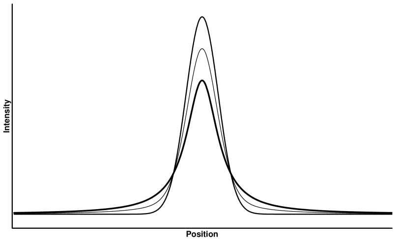
Figure 1.6: Graphs of Gaussian (highest peak), Lorentzian (lowest peak) and pseudo-Voigt profiles having the same parameters with a pseudo-Voigt mixing factor $m=0.5$.

The fit can be performed on the pattern as a whole or on selected regions or selected peaks which can be fitted together or separately. The procedure is based on minimising the difference between the observed and calculated profiles using normally a nonlinear least squares technique. The technique is required to minimise the second norm of the residuals given by

$$L_{2}=\sum_{i}w_{i}\left(y^{o}_{i}-y^{c}_{i}\right)^{2}$$ (1.5)

where $y^{o}_{i}$ and $y^{c}_{i}$ are the observed and calculated intensity at each step respectively and the summation index $i$ runs over all points in the range of the segment to be fitted. The weights $w_{i}$ are taken from the experimental error margins which in most cases are assumed to be in proportion to the square root of the observed count rate $y^{o}_{i}$ following a Poisson counting statistics [137, 44].

Curve-fitting is the most accurate method for extracting pattern parameters. Moreover, it is computationally efficient and relatively easy to implement and use. Curve-fitting is also very flexible since no detailed knowledge about the existing diffraction peaks is required, and hence it is the best choice when no information about the unit cell and symmetry are available. When the data quality is reasonable, the fitting can yield very accurate results. These results can then be used in subsequent processes such as quantitative phase analysis or structure determination, though the latter can be difficult when the pattern is too complex with severe peak overlapping. However, the method normally requires considerable time and effort and hence can be very slow and meticulous. Moreover, it is usually influenced by the results of an automated search routine or biased by the user judgment about the existence, position and profile of the peaks. The approach can also fail when the pattern suffers from serious overlapping, as the parameters of peaks occupying the same position cannot be determined by this type of fitting. In such cases, other fitting techniques such as whole pattern decomposition should be employed [31, 110].

Curve-fitting is the main method used in this study to analyse experimental data collected from a number of synchrotron facilities in various experimental settings and techniques. Curve-fitting is implemented in EasyDD as single, multiple, batch and multi-batch processes with high speed and efficiency. This made possible the analysis of huge data sets by fitting millions of peaks within hundreds of thousands of diffraction patterns in just a few hours. Examples of such large-scale processing and analysis of massive data sets are presented in chapters 4 and 5. Each peak is used as a signature for a particular phase that can be used to detect spatial and temporal distributions. Hence, EasyDD curve-fitting implementation offers a great support to highly important research areas such as dynamic phase transformation studies.

1.4.3 Two-Stage Method

This method for extracting information from powder diffraction patterns requires two-stages. In the first stage, the diffraction pattern is analysed to separate the peaks and peak clusters of the pattern into individual reflections to extract their parameters such as position and integrated intensity. In this stage, curve-fitting or whole pattern decomposition procedures, which do not require structural information, are usually employed. In the second stage, the individual reflection data are used for structure determination or for other purposes like strain and texture analysis. This stage includes the actual crystallographic calculations, which may involve either refinement by using an optimisation method (usually a least squares routine) or procedures like Fourier analysis or Patterson maps [79].

The two-stage method has been used in X-ray and neutron diffraction data analysis since early 1960s. The introduction of the Rietveld whole pattern refinement with its attractive features diminished the importance of the two-stage method and reduced its use. However, it is still in use in some applications that Rietveld refinement cannot substitute. Moreover, those who rejected Rietveld refinement [38, 127, 39] regard the two-stage approach as the only legitimate procedure for information extraction. The method has been constantly modified and extended to incorporate new developments mainly in peak deconvolution techniques. The method has a number of adaptations and interpretations which share this common general feature of a two-stage procedure [143, 42].

1.4.4 Whole Pattern Modelling

Modern powder diffraction heavily relies on pattern modelling techniques. Whole pattern modelling is based on fitting the whole diffraction pattern to a model characterised by a number of parameters and applying a refinement procedure, where ‘refinement’ means adjusting the model parameters to optimise the fit to the observed data. The best fit is quantified according to some predefined discrepancy indicator(s). In most cases, whole pattern modelling employs a nonlinear least squares procedure which requires sensible estimates of many variables. These normally include peak shape parameters, background contribution and crystallographic variables such as unit cell dimensions and atomic coordinates in the unit cell. Various standard indicators (figures-of-merit) are usually used to measure the quality of fit. Unlike curve-fitting, whole pattern modelling methods require knowledge of the structural parameters, or at least knowledge of the unit cell parameters, which may be difficult or impossible to obtain. Moreover, these methods are computationally demanding and usually case-specific and hence may not be suitable for use in batch processing of large quantities of data [125, 128].

There are two main approaches to the whole pattern modelling: structure modelling and pattern decomposition. In the first approach a background model and line shape functions are employed to fit the observed data with presumed crystallographic structural information, while in the second approach no such information is required. Rietveld refinement procedure [123, 124] is the known example for whole pattern structure modelling, while Pawley [108, 109] and Le Bail [90] procedures are the prominent examples for whole pattern decomposition. It is noteworthy that pattern decomposition techniques were introduced following the advent of the Rietveld method.

1.4.4.1 Whole Pattern Structure Modelling

As the peak intensities in the diffraction pattern depend on structural factors such as atomic type and their distribution within the unit cell, measurement of intensities allow quantitative identification of the phases involved and structure determination. In single crystal diffraction, the intensities can be measured, in principle at least, in a straightforward way. The measurement of intensities in the powder diffraction pattern on the other hand is more complex because of peak overlap and the involvement of complex sample and instrument factors. Due to these complexities, structural information from powder diffraction pattern is preferably obtained by a whole pattern structure refinement technique. The refinement starts by assuming a structural model with variable parameters which have to be tuned to achieve the best agreement between the observed data and the calculated values according to some statistical indicators. Background and profile models are also included alongside the structural model in the fitting procedure to account for non-structural factors contributing to the experimental pattern. Visual inspection and various figures-of-merit can be used to assess the quality of the fit [79, 3, 125].

The Rietveld Method is the most popular of powder diffraction pattern refinement techniques. The method is based on fitting the structural model directly to the total pattern of Bragg reflections. It extracts the maximum available information from the collected diffraction data. The Rietveld method is a procedure for structure refinement and not for structure determination. Therefore, a knowledge of the crystallographic space group symmetry and unit cell dimensions with approximate atomic positions is required as the method is not capable of creating a crystallographic structural model from first principles. In multi-phase samples, crystal structures of all individual phases must be known. The method also requires high quality experimental diffraction data and suitable functions to model peak shape and background contribution. In this regard the type of radiation source, sample quality, experimental settings and instrumental resolution play a crucial role and impose a limit on the complexity of the problem to be solved. For example, Rietveld refinement is more likely to succeed when using synchrotron diffraction data than when using data from domestic X-ray sources. In the Rietveld method a calculated full profile is generated and a refined list of parameters that best fit the experimental data are produced. The method relies on a least squares routine as a refinement minimisation technique. The solution should be inspected and assessed by some independent criteria if possible as an apparently successful Rietveld refinement may not be enough to prove the correctness of a crystal structure solution [124, 140, 26].

Although the Rietveld procedure was originally proposed for structure refinement, nowadays it is widely used for other kinds of analysis as well as structure refinement. The method can provide information about crystal and magnetic structures of single- and multi-phase samples, and determine the relative amounts of each phase in quantitative phase analysis from powder samples. The method can be used to provide a wide range of information about lattice parameters, atomic positions in the unit cell, fractional occupancy, thermal displacements, average crystallite size, average strain, preferred orientation, and so on. It is noteworthy that neutron powder diffraction is the technique that mostly benefitted from the invention of the Rietveld method because of the simplicity of peak shape produced by the relatively crude resolution of neutron diffraction instruments [146, 86].

In the literature of powder diffraction refinement there is a number of guidelines and recommendations that should be followed if good results are to be expected from the Rietveld procedure. These include recommendations about the sample, instruments, radiation source, data collection method, Rietveld refinement strategy and so on. It should be remarked that the refinement can lead to a wrong solution even when these guidelines are followed and the refinement converged with low $R$-values although the likelihood of this occurring is usually small. Apart from complying with the formalities of the refinement process, such as having good figures-of-merit, the resultant model should be sensible. Visual inspection and independent checks from other sources of information, when available, must also be performed [26, 98].

1.4.4.2 Whole Pattern Decomposition

Whole pattern decomposition or whole pattern fitting is a widely used method in diffraction pattern modelling. In many situations the crystal structure is unknown or is not of interest for the application in hand. In such cases, pattern decomposition can be employed to characterise the pattern and obtain the required parameters of the individual diffraction peaks. In this method the whole pattern is deconvoluted into individual Bragg components with no use of a structural model. A nonlinear least squares minimisation technique is usually employed during this process. The parameters that can be refined by whole pattern decomposition include, integrated intensity, integral breadth, peak position, full width at half maximum, unit cell parameters, shape factor and line asymmetry parameter. As a whole pattern modelling technique, pattern decomposition can produce accurate individual peak parameters even when the pattern contains severely-overlapped peaks. The quality of the fit is assessed using a number of figures-of-merit, as in the case of Rietveld refinement. The significant advantage of whole pattern decomposition is that it does not require a structural model of the phases. Furthermore, additional peaks can be included in the refinement to deal with impurities from unidentified phases [94, 141].

Whole pattern decomposition has a wide range of applications, for example in lattice parameter refinement. The method may be used within a two-stage procedure to extract unit cell and profile information. In this context, the Bragg intensities are obtained in the first stage where the positions of the individual peaks are constrained by unit cell parameters. These intensities are then used in the second stage as an input to a refinement process. A shortcoming of pattern decomposition is that knowledge of the unit cell parameters is required, and hence the method can be biased towards the user choice. Furthermore, it may not be applicable in situations where such information is not available. Although both curve-fitting and whole pattern decomposition are profile fitting procedures, each peak in curve-fitting is normally regarded as independent of the other peaks even when they are in the same cluster. Moreover, only a limited range of the diffraction pattern is usually considered in the fitting procedure. On the other hand, in the whole pattern decomposition all peaks of the pattern or a large number of them are considered simultaneously and fitted as a whole. As pointed out already, knowledge of unit cell parameters is required for whole pattern decomposition but not for curve-fitting. The best known methods in pattern decomposition are the Pawley and Le Bail techniques which are based on a least squares fitting procedure and are derived from the Rietveld method. Nowadays, various modifications to the Pawley and Le Bail procedures are in use, representing different approaches in extracting the required parameters from diffraction patterns.

1.4.4.3 Statistical Indicators and Counting Statistics

It is desirable in pattern modelling to have the ability to measure the quality of the fit as a whole by a single number. In the literature of powder diffraction, a number of standard statistical parameters have been proposed and used to monitor the convergence process and check the quality of the fit. They are used as indicators of how the refinement process is progressing and how good the final result is. These indicators are called functions-of-merit or figures-of-merit (FoM). Although these parameters are usually associated with the whole pattern structure refinement, they are more general and are employed in curve-fitting and pattern decomposition as well. The main FoM are the profile residual $R_{p}$, the weighted profile residual $R_{w}$, the expected residual $R_{x}$, the Bragg residual $R_{B}$, the structure factor residual $R_{{\bf F}}$ and the goodness-of-fit index $\chi^{2}$ [128, 80]. These are presented in Table 1.4.

Table 1.4: Statistical indicators for pattern fitting and refinement.

Statistical indicator	Definition
Profile residual	$R_{p}=\frac{\sum_{i}|y^{o}_{i}-y^{c}_{i}|}{\sum_{i}y^{o}_{i}}$
Weighted profile residual	$R_{w}=\left[\frac{\sum_{i}w_{i}(y^{o}_{i}-y^{c}_{i})^{2}}{\sum_{i}w_{i}{y^{o}_{i}}^{2}}\right]^{1/2}$
Expected residual	$R_{x}=\left[\frac{O-P+C}{\sum_{i}w_{i}{y^{o}_{i}}^{2}}\right]^{1/2}$
Bragg residual	$R_{B}=\frac{\sum_{k}|{I}^{o}_{k}-{I}^{c}_{k}|}{\sum_{k}|{I}^{o}_{k}|}$
Structure factor residual	$R_{{\bf F}}=\frac{\sum_{k}|\sqrt{{I}^{o}_{k}}-\sqrt{{I}^{c}_{k}}|}{\sum_{k}|\sqrt{{I}^{o}_{k}}|}$
Goodness-of-fit index	$\chi^{2}=\left[\frac{R_{w}}{R_{x}}\right]^{2}=\frac{\sum_{i}w_{i}(y^{o}_{i}-y^{c}_{i})^{2}}{(O-P+C)}$

In these relations, $y^{o}$ and $y^{c}$ are, respectively, the observed and scaled calculated intensities at step $i$ in the pattern, and $w_{i}$ is the corresponding observation weight, usually assigned the value 1/$y^{o}_{i}$ on the basis of counting variance, assuming $\sigma^{2}_{i}$ = $y^{o}_{i}$ according to Poisson statistical distribution, as given by Equation 1.6. $O$, $P$ and $C$ are the number of observations, the number of refined parameters in the calculated model, and the number of applied constraints, respectively. ${I}^{o}_{k}$ is the integrated observed intensity of reflection $k$, and ${I}^{c}_{k}$ is the corresponding calculated integrated intensity. The summation index $i$ runs over all data points measured in the experimental pattern, while the index $k$ runs over all independent Bragg reflections. As these indicators measure the agreement between the observed and calculated quantities, they must be closely monitored during the refinement. When the refinement is progressing in the right direction, they should gradually decrease and finally settle to a minimum when convergence is reached. If these figures-of-merit start rising, which is a sign of divergence, the refinement should be stopped and resumed after imposing suitable constraints on the refined parameters [73, 86, 146].

The profile residual $R_{p}$ is described as a true quantity because it is based on the discrepancies between the observed and calculated intensity values. Of these figures-of-merit, the weighted profile residual $R_{w}$ and the goodness-of-fit index $\chi^{2}$ are statistically the most meaningful indicators of the overall fit since the numerator contains the residual that is minimised in the least squares procedure. The goodness-of-fit index, which is inherited from the general statistics literature and not specific to diffraction pattern refinement, is used and quoted quite often in the powder refinement literature and considered as one of the most important and widely accepted figures-of-merit. The expected residual $R_{x}$ is used in the Rietveld refinement to quantify the quality of the experimental data. The structure factor residual $R_{{\bf F}}$ is biased towards the structural model, but it gives an indication of the reliability of the structure. This quantity is not widely used to monitor the refinement process. The Bragg residual $R_{B}$ is based on the intensities deduced from the model and hence is biased in favour of the used model. It is highly dependent on the procedure in which the observed integrated intensities are estimated, and may be described as an artificial quantity generated in order to get values similar to the single crystal and two-stage residual. However, $R_{B}$ is a quite important figure-of-merit in Rietveld refinement though it has little or no value in full pattern decomposition because only observed Bragg intensities are meaningful in both Pawley and Le Bail methods [80, 146, 98, 143, 110].

Regarding the counting statistics, in the literature of powder diffraction the count rate is usually modelled by a Poisson statistical distribution. Consequently, the statistical weights given to each observation $w_{i}$ are obtained from the experimental errors which are regarded to be proportional to the square root of the observed count rate $y^{o}_{i}$, that is

$$w_{i}=\frac{1}{\sigma^{2}_{i}}=\frac{1}{y^{o}_{i}}$$ (1.6)

where $\sigma^{2}$ is the statistical variance. This weighting scheme reflects only the statistical errors in the observed values with no consideration to the errors in the calculated values. The latter, which can arise from defects in the structural or profile models and from inadequacies in the computational technicalities, should be accounted for by other means. Other weighting schemes for modelling the experimental errors have also been proposed and used. Examples include unit weight, reciprocal square of the observed intensity, and modulus of the difference between observed and calculated intensities [3, 146, 137].

1.4.4.4 Optimisation Methods

To extract good information from powder diffraction patterns, good experimental data and careful modelling should be associated with a good fitting algorithm. In pattern fitting and refinement, an optimisation procedure is required to achieve and measure the proximity of the model to the observational data. The most widely used optimisation procedure is the nonlinear Least Squares (LS) residual method in its various realisations such as Gauss-Newton and Levenberg-Marquardt algorithms. Although the least squares algorithms are sufficient, they suffer from some serious problems and are not ideal in all situations. Therefore other methods have been developed and used in powder diffraction pattern modelling. The main rivals to the least squares as an optimisation procedure are the maximum likelihood and maximum entropy methods. These are closely related as they both rely on the same basic principle [114, 59, 58]. In the following, we discuss and compare these optimisation procedures as applied in the powder diffraction pattern refinement.

Least squares fitting is probably the most popular numerical method in science and the main technique used in powder diffraction as it is an essential element in most pattern refinement routines. It is widely used to determine the best set of parameters in a model to fit a set of observational data. Both whole pattern structure refinement (Rietveld) and whole pattern decomposition (Pawley and Le Bail), as well as curve-fitting procedures, are based on a nonlinear least squares technique to minimise the difference between the observed and calculated profiles. The refinement of large structures by least squares can fail because the required computational resources dramatically increase as the number of least squares parameters increase. In these cases, reduction techniques such as block matrix approximation may be employed where only diagonal blocks of the original least squares matrix are used. Theoretically, this should produce the same solution but with less accurate error estimates. Also least squares may suffer from numerical instabilities resulting in practical difficulties such as unexpectedly large values of goodness-of-fit statistics in some data sets and unrealistic estimates of standard deviations in the refined parameters. Although least squares can be used to refine any model, the suitability and validity of the model in the particular case are out of least squares scope and hence require independent justification [100, 128].

The maximum likelihood method was introduced as another possibility for pattern refinement of crystallographic structures to replace the classical least squares and overcome its limitations. The objective of the maximum likelihood method is to find a raw model that has the best chance to be improved by applying small steps to achieve full agreement between the observed and calculated models [118, 24, 57, 5].

The maximum entropy is another optimisation technique that has been used in crystallography and powder diffraction to replace least squares. For example, maximum entropy is employed in some powder diffraction studies to restore the lost phase angles. It is also used in the pattern refinement as a deconvolution procedure to determine the relative intensities of the overlapped reflections from first principles. The technique is found to be efficient with simulated profiles having various noise levels [46, 60].

Chapter 2 Software for Powder Diffraction

An overwhelming number of computer programs have been developed over the last few decades for processing and analysing crystallographic and powder diffraction data; most of them are in the public domain. For instance, Smith and Gorter [133] identified over 280 programs developed until 1990 for the analysis of powder diffraction data. These programs can be used for solving almost any kind of crystallographic and powder diffraction problem. The majority of these programs are free of charge for academic use and can be downloaded from the Internet directly or via links from dedicated websites such as CCP14 [36]. Others can be obtained from the authors on request or require a license. Each category normally contains a number of programs that vary in quality, licensing, sophistication, computational efficiency, documentation, user friendliness and so on. The list is substantially increasing in number and the quality is generally improving all the time, though the rate of growth varies from one area to another. In each category, some programs are optimised for solving certain types of problems while others are optimised for different sorts of problems. However, in this chapter we provide a glimpse into this huge and fast-growing field by presenting some categories of the available software with very few examples from each. Most of these example programs perform other functions; however they were included in the category that is more appropriate to the major type of tasks they perform.

2.1 Pattern Simulation

One way for interpreting the information in a measured powder diffraction pattern is to calculate a theoretical pattern from a structural model to simulate the experimental data. Digital patterns can be varied to account for different instrumental and experimental conditions normally present in a diffraction measurement. Reference data can be adjusted to match observational data for various purposes such as phase identification, quantitative phase analysis, sample condition tests and so on. One approach in pattern simulation is to take the integrated intensities, which are calculated from the crystal structure description, and create a diffraction pattern by calculating profiles for every peak and combining them to simulate the actual pattern. To generate diffraction patterns, sufficient information must be supplied by the user regarding the crystal, background, instruments, peak shape, and so on. The availability of simulated diffraction patterns has facilitated the indexing and verification of diffraction pattern analysis. However, in some complex experimental conditions the simulated pattern may not reflect all the factors involved and hence careful scrutiny is required [133]. An example for this category of software is RIETAN (by Izumi) [78] which is a whole pattern refinement program that can also be used for simulating X-ray and neutron diffraction patterns. Many other Rietveld refinement programs can also simulate powder diffraction patterns.

2.2 Whole Pattern Structure Refinement

The Rietveld method is the most popular of powder diffraction pattern refinement techniques. Consequently, there are many programs for doing this sort of structural refinement with a great diversity in all aspects. Among the most popular of these programs are FullProf (by Rodríguez-Carvajal), GSAS (by Larson and Von Dreele), TOPAS (by Coelho), LHPM-Rietica (by Hunter and Howard).

FullProf is a collection of crystallographic programs mainly developed for Rietveld structure refinement of neutron and X-ray diffraction patterns. FullProf, which is written in Fortran, can be used for analysing various experimental data such as magnetic and nuclear scattering, time of flight and constant wavelength neutron experiments, as well as X-ray data in energy and angle dispersive modes. The suite can be run from command line interface and from WinPLOTR or EdPCR graphic interface [126]. FullProf is one of the most reliable and widely used examples of software in crystallographic and powder diffraction analysis.

The General Structure Analysis System (GSAS) of Larson and Von Dreele is a set of programs for processing and analysing single crystal and powder diffraction data that are obtained with X-rays or neutrons. GSAS can handle these types of data simultaneously for a given structural problem. It can also handle powder diffraction data from a mixture of phases, and refine structural parameters for each phase. GSAS features a menu-driven editor ‘EXPEDT’ which is used to prepare all the input for the main calculations. The entire GSAS system is written in FORTRAN. It can run on Windows, Linux and Macintosh [87].

TOPAS is a powder diffraction analysis software distributed in commercial and academic versions. The program has a graphic user interface but can also run from command line interface and by text-based input files, i.e. scripts. Full graphic interface is available only with the commercial version. The academic version, which is not free, is run from text input files that store a sequence of commands. TOPAS is praised for its stability, reliability and smooth convergence. The program can perform pattern decomposition by Pawley and Le Bail procedures as well as Rietveld structure refinement for both X-ray and neutron in angle and energy dispersive modes. TOPAS is also capable of performing powder indexing and structure solution by simulated annealing [35]. The text editor jEdit, with its powerful macro language, may be used to drive and control TOPAS in text-input mode.

LHPM-Rietica is a Rietveld analysis computer program. The suite consists of the LHPM Rietveld program and Rietica which helps in controlling LHPM as well as creating and updating the structure input files. LHPM-Rietica is a Windows (95/98/NT) based program with a simple graphic user interface. The program can perform neutron and X-ray Rietveld and Le Bail refinement in constant and variable wavelength modes, simulation of diffraction data in these modes, data and refinement parameters plotting, background and region selection input, integrated Fourier plotting, and data editing. The program has a macro language, similar to Basic, which can be used for complex batch processing and programming. LHPM-Rietica can interact with GSAS and FullProf through data importing [75, 76].

2.3 Whole Pattern Decomposition

Most Rietveld refinement programs have the capability to do whole pattern decomposition by Pawley or Le Bail methods with the latter being the most common. Examples include GSAS, TOPAS, RIETAN, and LHPM-Rietica. The first two can perform both Pawley and Le Bail fittings, while the others can do Le Bail only.

2.4 Curve-Fitting

The method of curve-fitting with no knowledge of unit cell or structural parameters is based on decomposing the pattern into independent peaks using relatively simple profile models to extract the integrated intensity and other profile parameters. Usually, a limited range of the pattern is considered during this process. There are many curve-fitting programs, some are general purpose while others are specifically developed for powder diffraction. A prominent example of curve-fitting programs is Fityk [55] (by Wojdyr) which is free software with a graphic user interface. It can also be driven by a command line interface using text file scripts. The program runs under different platforms including Linux, Windows and Macintosh. Fityk is written in C++ language with Python bindings. Its main functionality is nonlinear fitting of analytical functions to a set of data points using a number of commonly used basis functions such as Gauss, Lorentz, Voigt, polynomials, and Pearson VII. It offers background subtraction with different nonlinear fitting methods. Fityk offers three optimisation methods (Levenberg-Marquardt, Genetic Algorithms, and Nelder-Mead simplex) with error modelling and application of constraints.

A second example of curve-fitting programs is CMPR [34] (by Toby) which is a platform-independent multipurpose package for analysing, visualising and manipulating powder diffraction data. As well as curve-fitting, the program can perform manual- and auto-indexing, and offers some handy features such as graphic display and manipulation of $hkl$ lines. A third example is Xfit (by Cheary and Coelho) which is used by powder diffraction community [36]. EasyDD can also perform curve-fitting in single, multiple, batch and multi-batch modes.

2.5 Search-Match

Search-match programs require a database of diffraction patterns such as Cambridge Structural Database and Powder Diffraction File. Some of these databases have their own search-match programs. The databases for search-match routines are generally based on X-ray diffraction patterns. Search-match programs vary in their underlying search algorithm, speed, reliability, and so on. Some programs are capable of examining, in a few seconds on a normal computer, tens of thousands of powder diffraction patterns and proposing a list of candidate patterns to match the unknown pattern. The results of the search-match depend on the quality of the observational data, the quality of the database, the search-match algorithm, and the criteria used in the search. Matches are usually ranked using a figure-of-merit where a large figure-of-merit normally means good match. It is quite possible that all the suggested patterns are not suitable, and hence the user should accept or reject the proposed patterns based on clear evidence [143].

Most existing search-match programs do not use the full profile data. Instead, they rely on simplified patterns in which the full diffraction profile is reduced to a set of the strongest peaks. The main advantage of this reduced approach is high speed and less computer resources especially when using large databases. Most search-match programs that are in the public domain are commercial. An example of the search-match software is $d$SNAP (by Barr, Gilmore, Dong, Parkin and Wilson) which is a graphic user interface program for automatic classification and visualisation of the results of database searches using the Cambridge Structural Database (CSD) [15]. Another example is Portable Logic Program (by Toby) which can be used for searching the International Centre for Diffraction Data (ICDD) database. The program is currently incorporated within the CMPR suite [34].

2.6 Structure Visualisation

Visualisation of crystal structure means displaying the arrangement of atoms, ions, and molecules in the unit cell, usually in 3D space with or without unit cell outlines. The atoms are normally represented by coloured spheres with their sizes being in proportion to the atomic sizes. The plot can usually be scaled, translated, rotated, zoomed and manipulated in various ways with possible labels and explanatory comments. The software may enable the user to measure and display things like unit cell axes, angles, distances, and torsion angles. The software usually reads the structure from raw data files with a specific format. Alternatively, the data can be obtained and mapped directly from within the program following a structure solution or structure refinement process. These programs usually recognise several data formats and may be able to import and export between them. Structure visualisation can be a great aid in comprehending and checking the solution. Examples of structure visualisation programs are Mercury (from Cambridge Crystallographic Data Centre), DRAWxtl (by Finger, Kroeker and Toby), and Materials Studio (from Accelrys).

Mercury CSD, which is part of the Cambridge Structural Database System, is a popular program for visualising crystal structures in 3D using a range of visualisation options and display styles. The program can read crystallographic structural data in various formats. It is written in C++ language with an object oriented nature. Mercury can display multiple structures simultaneously and perform least squares overlay of pairs of structures. It can also do various transformations such as rotation and translation [96, 27].

DRAWxtl is an open source computer program for crystal structure drawings. It produces standard graphical representations such as spheres, ellipsoids, bonds and polyhedra. The drawing output is produced either in the form of an interactive screen representation, or as Virtual Reality Modelling Language (VRML) files. The program is supported on a variety of platforms such as Windows, Mac, Linux and other Unix distributions. It has the ability to plot incommensurately modulated and composite structures. It can also produce input files for the Persistence of Vision Raytracer (POV-Ray) rendering program to create high quality images [53].

Materials Studio is a commercial multi-module software environment for molecular modelling, simulation and visualisation. The program is designed for structural and computational researchers in chemistry and materials science. It provides tools for modelling crystallisation processes and crystal structure. It can also be used for studying polymer properties, catalysis, and structure-activity relationships [97]. It should be remarked that many crystallographic and powder diffraction programs are capable of producing visual images of the resolved structures. Several examples can be found in the category of whole pattern refinement programs such as TOPAS.

2.7 Data Visualisation

The purpose of data visualisation is to present numerical and abstract data in visual form. Two main aspects of these visualisation techniques are colour-coding, and graphic plotting in 2D and 3D space. For example, it is common practice in powder diffraction to use 2D stack plots or 3D surface plots of a series of diffraction patterns in dynamic phase transformation studies. Another common form of visualisation in powder diffraction is the 2D tomographic colour-coded images of the total intensity of pixels in tomographic imaging studies. These tomographic images are also used to display the integrated intensity of a particular peak in phase identification investigations. This sort of visualisation provides a brief, comparative and informative glimpse of certain parameters of the individual data sets. This enables the user to perform summary analysis and make critical judgments about the next step in data collection and analysis. This kind of visualisation is very important in some situations such as collecting data from synchrotron facilities where beam time is scarce and should be exploited maximally, or when the available computational resources are limited and do not allow for detailed analysis.

These days many computer programs have a kind of data visualisation capabilities such as plotting the measured and refined diffraction patterns. Most whole pattern structure refinement and whole pattern decomposition programs, such as GSAS and TOPAS, have this visualisation capacity. Matlab scripts are also in common use by the scientific community to perform this sort of visualisation. EasyDD includes several visualisation capabilities such as 2D pattern plotting, 3D surface plotting and 2D colour-coded tomographic imaging. The program can also create images in single and multi-batch modes and save them as image files to the computer permanent storage.

2.8 Indexing

Indexing of powder diffraction patterns means the determination of $hkl$ indices of each reflection, the dimensions of the unit cell and the crystal symmetry. This is an essential and limiting step in an ab initio structure determination from powder diffraction data. A list of indexed intensities obtained from an indexing procedure may be used, for example, as a starting point for the application of direct methods. There are several indexing methods that vary in their speed, efficiency and reliability. These include zone indexing, trial, dichotomy, and Monte Carlo methods. The efficiency of most powder pattern indexing software significantly deteriorates in the presence of impurity lines [86]. An example of indexing software is Crysfire (by Shirley et al) which is a family of programs interconnected by a set of interlocking scripts in the form of batch files. Its role is to act as an expert system to allow indexing of powder diffraction patterns quickly and smoothly by non-specialists [132]. Another example is Supercel (by Rodríguez-Carvajal) which is for indexing of super-cells and incommensurate structures. A third example is Chekcell (by Langier and Bochu) which is an indexing program for unit cell and space group assignment [36]. As indicated already, CMPR (by Toby) can also perform manual- and auto-indexing.

2.9 Unit Cell Refinement

On indexing a powder diffraction pattern, the unit cell parameters ($abc,\alpha\beta\gamma$) become known approximately. These parameters may then be refined by a least squares fitting routine taking into account constraints due to the crystal system symmetry. Unit cell refinement of standard materials is also used to check instrument and sample alignment. In principle any whole pattern refinement program can do a kind of unit cell refinement [109]. An example of dedicated unit cell refinement programs is LAPOD (by Langford) which performs a least squares refinement of cell dimensions from powder data using Cohen’s method. Another example is CELREF (by Laugier and Bochu) which is a unit cell refinement program within the LMGP suite that can calculate lines based on the space group and auto-select and auto-match calculated-to-observed peaks [36].

2.10 Structure Solution

There are several programs that can perform crystal structure determination from powder diffraction data. These programs use various structure solution techniques such as direct methods, simulated annealing and Monte Carlo. One example is EXPO (by Altomare et al) which is the integration of two programs, one for whole powder pattern decomposition and the other for the solution and refinement of crystal structures [4]. Another example is ESPOIR (by Mileur and Le Bail) which is a reverse Monte Carlo and pseudo simulated annealing software for ab initio crystallographic structure determination from a random starting model or from molecule location [101].

2.11 Utility Programs

These programs do various jobs which are essential for managing, processing and analysing diffraction data. These jobs include merging files, data format conversion, mass-scale text replacement, GUI management, background removal, peak finding, graphical interfacing, specimen displacement, aberration correction, smoothing, peak offset determination, plotting, and so on. The diversity and usefulness of these utilities cannot be overestimated. Examples of this category are DLConverter (by Smith and Sébastien), Powder4 (by Dragoe), and PowderX (by Dong).

DLConverter is a program with a simple graphic user interface developed at Daresbury SRS for conversion of large amounts of diffraction data produced by modern fast detectors between different formats. The program has an excellent batch processing capability and hence can be regarded as an example of batch processing programs [135]. Powder4 software is a collection of tools developed for X-ray powder diffraction. Its capabilities include management (e.g. merging) and conversion of data files between various formats [47]. PowderX is another software developed for the analysis of X-ray powder diffraction patterns. It has a number of useful processing utilities such as smoothing, background removal and format conversion [45]. EasyDD can also be included in this category as it can be used, for example, for data format conversion.

2.12 Batch Processing

There are many programs that do various jobs in batch mode to perform essential duties in managing, processing and analysing data. These include several powder diffraction programs that can be driven in batch mode and hence can be used for large-scale processing and analysis. An example of these programs is PolySNAP packages (2 and M) [113, 14] which are high throughput commercial software for analysing large data sets. They are designed to match and analyse patterns utilising their full profiles, and hence allowing for quick and accurate identification of samples. Their functionalities can be automated for high throughput analysis to allow the interrogation of large data sets (up to 1500) in a single run. PolySNAPs provide quantitative phase analysis of mixed samples using a non-Rietveld approach, and employ several novel statistical methods with a user-friendly graphic interface. The analysis results are summarised and visualised using a flexible graphic output.

Among the prominent powder diffraction programs that can run in batch processing mode is FullProf. It is also reported that GSAS can be driven in batch mode by other purposely-written programs or scripts. EasyDD is another example of batch processing software, as most of its functionalities are implemented in batch and multi-batch modes, as will be explained in chapter 3.

2.13 Data Preparation and Pretreatment

These programs process raw data produced by detectors and acquisitions systems as a first step for further processing and analysis. Examples of preparation processes include introducing systematic error corrections, squeezing binary image files to extract ASCII numeric data, and changing the dimensionality of data by converting 2D diffraction patterns to 1D. An example of this category of software is Datasqueeze [41] which is a commercial program with graphic user interface that runs on a number of platforms. It is used for processing and analysing data from 2D X-ray diffraction detectors such as wire, image plate, and CCD devices. The program can run in batch mode to do various jobs, and hence it is also an example of batch processing programs. The batch mode jobs include converting binary image files, such as EDF which contain Debye-Scherrer rings on 2D image plates, to 1D powder patterns in ASCII numeric format.

Another example of this category is FIT2D [54] which is free software written in Fortran language for Windows and Unix platforms. It is both a general purpose and specialist 1D and 2D program for data reduction and analysis. It is used on most beamlines of the European Synchrotron Radiation Facility and by other research groups around the world. The program supports processing of 1D and 2D data, and recognises different detector types. It is used to convert data obtained from 2D detectors, such as image plates, to 1D powder patterns, usually as intensity versus scattering angle. FIT2D has a graphic user interface with command line capabilities and macro language which may be used for automating repetitive processes. Most FIT2D functionalities, can be performed in batch mode to process large data sets in a single run, and hence it is another example of batch processing programs. A third example of this category is EasyDD which has the capability of EDF binary image squeezing. It also has the capability of manipulating, correcting and performing initial analysis on SRS 16.4 data and binary files from HEXITEC multi-TEDDI detectors.

Chapter 3 EasyDD Program

The idea of high throughput software emerges from the need to process huge quantities of data in a consistent and repetitive manner using automated procedures. The demand for high throughput processing capabilities in scientific research has substantially increased in recent years. One reason is the availability of bright radiation sources, such as synchrotron and neutron facilities, which facilitate the collection of massive amount of data in short periods of time. Another reason is the essential improvement in data acquisition technology, and the more radical anticipated improvement in this technology such as multi-TEDDI detectors which are under development for high energy X-ray applications. The revolution in digital technology has also contributed to the mass accumulation of data and encouraged this phenomenon. This is due to the growing use of automated and computerised data collection techniques on one hand, and to the availability of vast electronic storage with massive processing computational power on the other.

The principal objective of EasyDD project was to develop a computer code for batch processing, visualisation and large-scale analysis of huge volumes of spectral data, mainly those obtained from synchrotron radiation sources for powder diffraction applications. Such a utility greatly assists studies on various physical systems and enables far larger and detailed data sets to be rapidly interrogated and analysed. At the start of EasyDD project a number of general objectives were set; the main ones were

• The program must be user friendly to minimise the time and effort required to learn and use. A graphic user interface was therefore adopted in favour of a command line interface although the latter is more common in scientific computing and much easier to develop.

• It should be capable of handling several common data file formats including a generic format so that the program can be used for processing data produced by different detectors and acquisition systems.

• The program must lend itself to future development to meet the ever-increasing demand on data processing and analysis capabilities. Therefore, it should be built on a continuously developing technology to keep in pace with the advancements in computing and GUI technology.

• It must be optimised for the commonly available computational resources; most importantly CPU time and memory. The program therefore tries to set the limits of its data processing capacity to the limits of the available computational resources.

EasyDD can be defined as a high throughput software to manage, process, analyse and visualise scientific data in general and synchrotron X-ray data in particular. The name ‘EasyDD’ comes from the original name ‘EasyEDD’ which was adopted for historical reasons as the software was developed initially for the users of the energy dispersive diffraction SRS station 16.4. As the program eventually evolved to be more general and can be used for processing ADD data as well as EDD data, the name ‘EasyDD’ was adopted to reflect this extension. In fact, currently there is no restriction on the program being used for general applications not related to synchrotron and powder diffraction, as the program is capable of processing any data having the correct format. One of these formats is a generic $xy$ style which can be used for all-purpose data. The program, which consists of about 30000 lines of code, is written in C++ language and uses a hybrid approach of procedural and object oriented programming. Its main attribute is the ability to process large quantities of data files with ease and comfort using limited time and computing resources. Most EasyDD algorithms are optimised for speed and hence it can be rightly described as ultra-fast high throughput software.

EasyDD combines Graphic User Interface (GUI) technology, such as dialogs, tooltips, colour coding, and context menus, with standard scientific computing techniques. Its resources include the standard C++ library, Qt toolkit [115] and its extension QwtPlot3D [116] for GUI design, with numerous algorithms, functions and techniques. The ultimate objective of EasyDD is to become a workbench for spectral data analysis. In EasyDD, the main data are stored in a 3D vector where the basic unit is a ‘voxel’ object in which all information relevant to an individual data set are stored. As a user-friendly feature, most components have memory, i.e. the settings are saved on exiting the program. Another user-friendly feature is that the components have explanatory tooltips which give brief description of the function (e.g. button tooltips) or reveal information related to the data represented by that component (e.g. tab tooltips).

Currently, eight input data formats are supported: generic $xy$, MCA of the Diamond synchrotron, MCA of the ESRF, ERD, LUCIA, HEXITEC, SRS 16.4, and EDF files. The first is a simple $xy$ format where the first column in the file contains the $x$ values (e.g. energy or channel number or angle) while the second column contains the $y$ values (e.g. intensity or count rate). The second is the MCA format of the Diamond Light Source [43]. The file contains the $y$ values (number of counts) only, as a function of an implicit channel number, with possible redundant header and footer lines. The third is the MCA format of the European Synchrotron Radiation Facility [50]. The file has only headers to be ignored, and the first data line starts with ‘@A’ with each 16 data entries occupying a single text line ending with backslash ‘$\backslash$’. Again, the data in the ESRF MCA files are number of counts versus an implicit channel number. The fourth is the format of the ERD multi-pixel 2D detector of the University of Manchester. The fifth is the format of the LUCIA beamline at the SOLEIL synchrotron [95]. The sixth is the format of the HEXITEC [72] multi-pixel 2D detector. The seventh is the format of the data files obtained from station 16.4 of Daresbury Synchrotron Radiation Source [138] in EDD mode. The eighth is the format of the EDF image files of the ESRF. The code can be easily extended to support other data formats.

One of the main functionalities of EasyDD is to read files from data sets collectively and map their information on GUI components. What is required for this operation is to deposit the files in a directory and invoke the relevant reading function. In the case of the SRS, where the data files have a highly structured format, the files are read and automatically recognised (i.e. SRS, scalars and vectors), and therefore non-SRS files in the source directory are identified and ignored. For the other formats, the file extension is used for type recognition, and hence no foreign files of the same extension should be mixed. On reading the files, the data are stored in memory and mapped on a 2D colour-coded tab. Multiple tabs from different data sources and of different data types can be created at the same time. The tabs can also be removed collectively or individually in any order. On removing a tab, all the data belonging to that tab are erased from memory and hence lost permanently. The remaining tabs will be relabelled to reflect the current state.

In the following sections we outline the main components of EasyDD.

3.1 Main Window

This is a standard GUI dialog with menus, toolbars, a status bar, context menus and so on. The basic functionality of the main window (seen in Figure 3.1) is to serve as a platform for accessing and managing the other components.

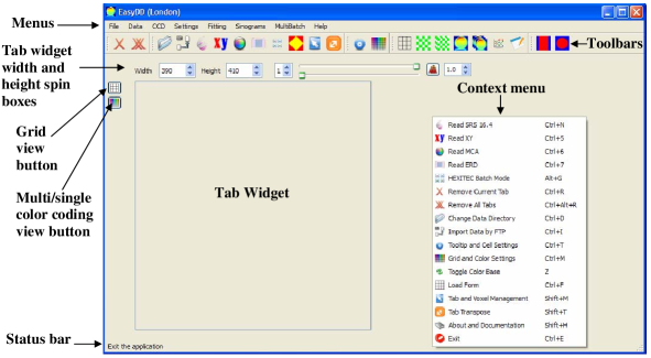
Figure 3.1: EasyDD main window.

3.1.1 Menus

The main window has several menus which provide access to the program functions. These menus, some of which have submenus, contain all the main items of the program. The keyboard shortcut for each item is shown on the right of the item title, and an icon characterising the item is displayed on the left of the title.

3.1.1.1 File Menu

This menu (Figure 3.2) includes the following items

• Remove Current Tab (): to remove the current tab and erase data from memory.

• Remove All Tabs (): to remove all tabs and clean the memory.

• Save Tab Image (): to save the image of the current tab in png format.

• 3D Graph (): to plot a 3D graph of the current tab.

• Exit (): for closing the main window and hence exiting the program. All saveable settings will be saved to the disc, and hence activated on the next launch of the program.

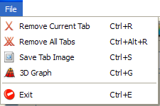
Figure 3.2: The main window File menu.

3.1.1.2 Data Menu

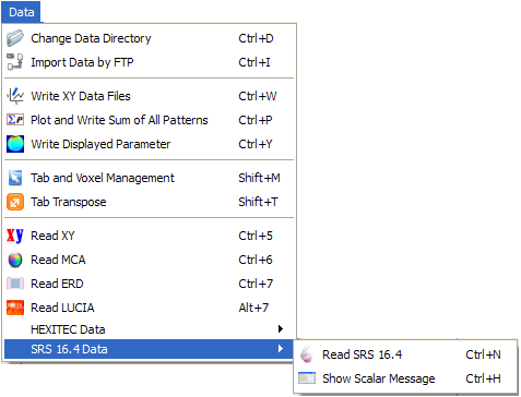
Figure 3.3: The main window Data menu.

This menu (Figure 3.3) includes

• Change Data Directory (): to launch ‘Browse for Folder’ dialog (Figure 3.4). From this dialog the user can navigate to the folder of choice where the required input data files are stored. As a user-friendly feature, the program has default directories for data reading when the program starts. These default directories are: ‘DataESRFXY’ for $xy$ data type, ‘DataMCA’ for MCA, ‘DataHEXITEC’ for HEXITEC, ‘DataSRS164’ for SRS 16.4, and ‘DataEDF’ for EDF. The multi-batch functions in MultiBatch menu also have a default directory called ‘MultiBatch’. On changing the data directory by using ‘Change Data Directory’ function, all default directories are suspended and the newly selected folder will become the default directory for all functions that require reading input data.

  

  Figure 3.4: ‘Browse for Folder’ dialog.

• Import Data by FTP (): to launch the FTP dialog (Figure 3.5). This dialog (Figure 3.5) is for importing files by File Transport Protocol (FTP). The dialog has three line editors: ‘Ftp server’ to input the address of the remote server, ‘Username’ and ‘Password’ to input these attributes. The ‘Connect/Disconnect’ push button is for connecting/disconnecting to the server after entering valid data. On connecting to the server, the folders and files on the server root directory appear on the list widget beneath the line editors. A folder can be opened and its contents inspected by double-clicking on its icon in the list widget. On pressing the button () next to the first line editor, the list widget view returns to the parent directory. A file can be downloaded from the remote server by selecting it first followed by pressing the ‘Download’ button. The ‘Quit’ push button is used to close the FTP dialog. The current functionality of the FTP utility is primitive and hence requires major development.

  

  Figure 3.5: FTP dialog.

• Write XY Data Files (): to write the data of the current tab to text files (one file of *.txt type for each voxel) in generic $xy$ format. The files of each tab are saved to a folder named ‘xyDataTab$N$’ where ‘$N$’ stands for the tab number. The naming of files follows the style ‘T$t$R$r$C$c$’ where $t$, $r$ and $c$ are the indices of tab, row and column respectively. The indices have constant width (e.g. ‘01’ for ‘1’ as a 2-digit number) to keep the order when re-reading these files. This routine facilitates saving, converting between data types, and exporting to other applications for further processing such as visualisation.

• Plot and Write Sum of All Patterns (): to plot the sum of all patterns in the current tab and write the numeric data to an $xy$ text file named ‘spectraSumTab$N$’ where $N$ is the tab number. This function is based on the assumption that all common channels of the patterns of the current tab voxels share the same $x$ coordinates. However, it is general with regard to the number of data points in each pattern and hence it works even when they are different in size by summing the existing channels and plotting the result for the maximum number of channels. The curve-fitting capacity of the plotter used in this function is disabled.

• Write Displayed Parameter (): to write the data of the displayed parameter (e.g. FWHM and total or integrated intensity) on the current tab to a file named appropriately (e.g. Tab$N$_Intensity for intensity) to indicate the written parameter. The value of the parameter of each voxel in the tab will be written. These values are structured in a 2D matrix depicting the dimensions of the current tab.

• Tab and Voxel Management (): to perform one of 12 functions for manipulating rows, columns and cells in the current tab. These functions are: delete row, delete column, set cell to zero (i.e. zero $x$ and $y$ coordinates), copy cell (source to destination), exchange cells, delete cell, rotate row anticlockwise, rotate row clockwise, rotate column anticlockwise, rotate column clockwise, exchange rows, and exchange columns. The copy operation is performed by copying the source (first cell) to the destination (second cell). An input data file called ‘TabManagement’ is required for tab and voxel management. To perform each of these functions, a specific keyword is required to identify the operation. The keyword should be followed by the indices of rows and/or columns to identify the item(s) that these operations are applied upon. On the first use of this menu item in the current session, a message (seen in Figure 3.6) appears to display the available functions and their keywords in the required format in the input file with an example of the required indices. If this message is needed again, a new session, possibly with another instance of the program, should be launched. The appearance of this message only once in each session is for the purpose of keeping the user informed with minimum inconvenience. When the input file contains more than one entry (i.e. a keyword with its parameters) the program will read the input file line by line and execute each line until it reaches the end of the file. Each line should contain a single keyword with its parameters as the rest of the line will be ignored and hence can be used for storing comments or entries that may be needed in the future. It should be remarked that all these functions are available in the tab context menu (with no need for an input file) by right-clicking on the current tab and choosing the appropriate option. In this case the current cell, row or column is identified by the click position. If a second item (cell, row or column) is required, as in the case of copy and exchange functions, the user will be instructed to click on the second item. Although the use of a context menu is more convenient, the advantage of performing tab and voxel management through an input file is to execute a series of these operations in a single run.

  

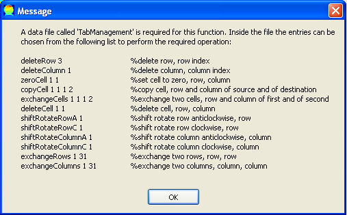
  Figure 3.6: Tab management message.

• Tab Transpose (): to transpose the current tab, i.e. exchanging rows and columns.

• Read XY (): to read data files that have an $x$ value as a first entry and a $y$ value as a second entry in each row. The rest of the row, which may contain other data such as an error index, will be ignored. Each file should contain data for a single voxel represented by a single tab cell. The process starts with the appearance of a dialog (Figure 3.7) from which the user can choose the number of rows and columns in the tab. This is followed by the ‘Change File Order’ dialog (Figure 3.8) from which the user can change the order of reading files or delete non-required files. The order of files can be changed by first selecting a file, then moving it up or down in the list using the ‘Up’ and ‘Down’ push buttons. Similarly, a file can be deleted by selecting it first followed by clicking ‘Delete’ button. It should be remarked that the reading operation will proceed only when the source directory contains sufficient number of data files. This is also true for other functions that require reading a certain number of data files from a source directory.

  

  Figure 3.7: XY dialog.

  

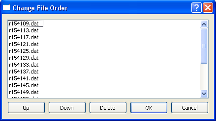
  Figure 3.8: Change File Order dialog.

• Read MCA (): for reading MCA data files. There are two supported MCA formats, as explained on page 3. In both cases, the process starts with the launch of the ‘MCA’ dialog (Figure 3.9) from which the user determines the number of rows and columns in the tab and the number of header and footer rows to be ignored. This is followed by the ‘Change File Order’ dialog (Figure 3.8) as in the case of an XY reading. It is noteworthy that for the ESRF MCA files the number of footers should be set to zero to avoid ignoring valid data entries.

  

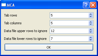
  Figure 3.9: MCA dialog.

• Read ERD (): for reading and mapping data files of the ERD detector. Each row in these files corresponds to an event taking place, i.e. a photon being detected by a specific pixel. The data in the rows consist of 5 columns. The first column contains the value in volts of the energy of event. The second column contains the index of the pixel in which the event took place. The pixels are indexed by a 2D array that depicts the physical layout of the detector channels. The third column contains a reference voltage used by the detector electronics. The fourth column identifies the frame in which the event took place. The fifth column contains a Boolean flag for data validation (‘1’ for valid and ‘0’ for invalid). In the current implementation of this function, the third and fourth columns are ignored. Because the energy is not quantised, a binning process is applied before creating the spectrum. The bin size is determined by the user, and is fed to the program through the map file which is outlined next.

  On invoking this function, a dialog appears to enable the user to choose the ERD data file to be read and mapped. This operation requires a map file called ‘ERD.map’. The map file contains the following data: number of rows, number of columns and voltage bin size. This is followed, on another text line, by the channels index map which mimics the physical layout of the 2D detector, as seen in Figure 3.10.

  The program ignores all the lines with invalid data, i.e. those whose Boolean flag on column 5 is 0. All the valid lines with the same pixel index (as given on column 2) are then grouped together and the energies (as given on column 1) for each pixel are processed as spectra. The $x$ values of these spectra are the bin numbers while the $y$ values are the number of counts, i.e. the number of events in a specific bin. The pixels are then mapped on a tab with the normal colour coding, tool tips, 2D and 3D visualisation, curve-fitting capability and so on, like other data formats. When a channel has less than three events, its cell on the tab is marked with white. The routine is general regarding the detector dimensions provided that a correct map file is supplied.

  

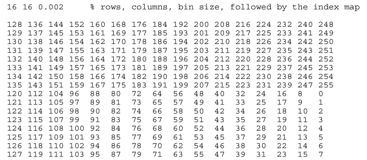
  Figure 3.10: A sample of an ERD map file for a $16\times 16$ detector.

  

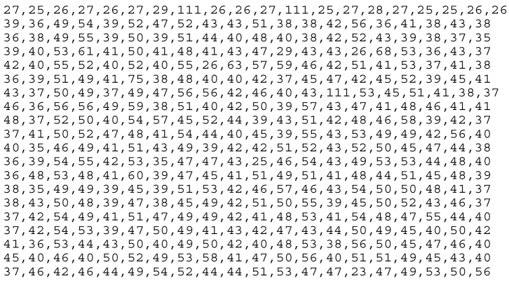
  Figure 3.11: A sample of a HEXITEC thresholds file for a $20\times 20$ detector.

• Read LUCIA (): for reading and mapping data files obtained from LUCIA beamline at SOLEIL synchrotron [95]. The file contains 960 patterns, each with 4000 channels. The patterns are arranged in columns, where each entry in these columns represents the intensity of the channel as a function of an implicit channel number. The user has the option to display these 960 patterns in a single row or as 32 rows times 30 columns on the EasyDD tab widget.

• HEXITEC Data: for reading and mapping data files obtained from the HEXITEC detector of Rutherford Appleton Laboratory. The data from the HEXITEC 2D detector is written as a continuous list of 16 bit values to a binary file. Each file contains a number of frames of data. A single frame contains $N=\mathcal{R}\times\mathcal{C}$ values where $\mathcal{R}$ and $\mathcal{C}$ are respectively the number of rows and columns of pixels in the detector. Each pixel in the detector has a different pedestal (offset) level. Therefore, a list of $N$ pedestal values should be provided in an independent file called ‘pedestals.txt’. Also the noise level on each pixel is different. Therefore, another file called ‘thresholds.txt’ should be provided to define the noise threshold (i.e. upper noise limit) of each pixel. These thresholds may require scaling by the use of a user-defined constant multiplier. To discriminate between the different data file formats, the program recognises the HEXITEC raw data files by the *.dat extension. The pedestal and threshold values should be positioned in their files in a 2D matrix to mimic the physical layout of the corresponding pixels in the detector. The neighbouring values in each row should be separated by a comma ‘,’. An image of a sample threshold file is shown in Figure 3.11. The other data are obtained from a dialog, seen in Figure 3.12. These data include the number of rows and columns, the thresholds multiplier, the number of bins, the minimum and maximum limits, a Boolean flag to run the end-of-frame algorithm, a Boolean flag to run charge-sharing algorithm followed by another flag for keeping/removing charge sharing events, and a Boolean flag to subtract from pedestals or ignore them. Apart from the *.dat binary files, all the other input data files should be located in the same directory as the program.

  

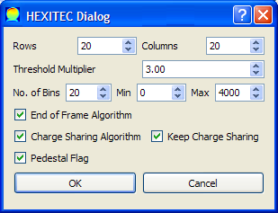
  Figure 3.12: HEXITEC dialog.

  Currently, the program can process the HEXITEC detector data in five modes:

  1. HEXITEC Generic Mode (): the raw data are read from a single *.dat binary file and mapped on a tab where the patterns represent uncorrected intensity as a function of frame number. This mode is normally slow and requires considerable memory space as the number of frames is usually very high (210000). This mode is useful for carrying initial checks on the raw data. For this mode, only the *.dat binary file and the number of rows and columns, which are obtained from the HEXITEC dialog, are required.

  2. HEXITEC Single Mode (): the program reads the raw data from a single file and corrects the individual entries by subtracting these entries from the corresponding pedestals. These corrected data are then compared to the corresponding threshold noise and the entries that fall below the threshold are discarded completely. The data which are below the minimum limit or above the maximum limit are also removed. The remaining data of each pixel are then binned into a histogram according to their values. This histogram, which can be plotted on the 2D plotter like other data formats, represents the number of events as a function of bin number. In addition to the raw data file, the pedestals and thresholds data files are required for this mode of operation. The other data (rows, columns, threshold noise multiplier, number of bins, minimum and maximum limits) are obtained from the HEXITEC dialog. The bins have equal width obtained by dividing the range (i.e. maximum minus minimum) by the number of bins.

  3. HEXITEC Batch Mode (): the raw data from multiple *.dat binary files are read and processed sequentially as in the second mode, but the results of these individual files are collectively displayed on a single tab. The histograms of the voxels in this tab represent the combined results of the individual files obtained by summing up these files. The program uses a default directory called ‘DataHEXITEC’ as a data source, unless the user has directed the program to another directory. All raw data files found in the source directory are read and processed. The other input files (i.e. ‘pedestals.txt’ and ‘thresholds.txt’) are expected to be in the directory of the program. Other required parameters are obtained from the HEXITEC dialog. In this mode, end-of-frame and charge sharing algorithms can be applied. Currently, the HEXITEC batch mode can run according to one of three options: end-of-frame with charge-sharing, end-of-frame without charge-sharing, and neither, i.e. charge sharing can be applied only with end-of-frame. It should be remarked that batch mode can run on a single file as well as multiple files.

     Note about the end-of-frame algorithm: when a pixel has an event in frame $N$ the user may want to ignore that pixel value in frame $N+1$. The end-of-frame algorithm identifies these pixels and applies this correction.

     Note about charge sharing algorithm: the voltage (signal) generated by a single X-ray photon in the HEXITEC detector can be shared between up to four neighbouring pixels. The reason is that a charge generated by an X-ray photon can be detected by more than one pixel. The purpose of the charge sharing algorithm is to identify and correct such charge sharing events. Charge sharing has two options: either allocate the event to a single pixel (i.e. the one with the largest voltage) or remove charge sharing by setting the voltage of all pixels involved in charge sharing events to zero and hence removing these events. Charge sharing corrections are conducted after removing the pixel offsets and the end-of-frame corrections, but before the data reduction.

  4. HEXITEC Batch Mode with Energy Calibration (): this is similar to the previous item (i.e. HEXITEC Batch Mode) but with performing linear energy calibration to the data by matching spectral peaks to their known energy. The energy calibration is used to convert the raw data from the detector into energy values as they are read into EasyDD. The calibration uses a linear relation given by:

     $$E(x,y)=m(x,y)X(x,y)+c(x,y)$$ (3.1)

     where $E(x,y)$ is the calibrated value (in keV) for the pixel in row $x$ and column $y$ from the raw data $X(x,y)$ with linear calibration coefficients $m(x,y)$ and $c(x,y)$. The calibration coefficients are provided in two text files (‘m.txt’ and ‘c.txt’) each containing an array of $m\times n$ values (where $m$ and $n$ are the number of rows and columns respectively) similar to the format of the thresholds and pedestals files. Energy calibration is performed after low energy threshold cutting and before charge sharing correction/discrimination. A message appears at the beginning to inform the user about the nature of this function and the sequence of operation. In the case of end-of-frame with charge-sharing, an output file called ‘Stat.txt’ which contains the number of valid and discarded events is created. It should be remarked that this function requires an input file called ‘binNumber2.txt’. This file (which was temporarily introduced for the purpose of testing) contains the number of bins which should equal or exceed the number of bins in the HEXITEC dialog.

  5. HEXITEC Batch Mode with Energy Calibration (New Format) (): this function is similar to the previous one (i.e. HEXITEC Batch Mode with Energy Calibration) but uses the new HEXITEC data format. In this format, the binary data files of *.dat type contain spectral data for a number of frames. The sequence ‘255 255 255’ is used to signify a new frame. This is followed by the frame index which is a 48-bit integer. A new row is signified by the sequence ‘0 192’, which is followed by the row index (8-bit), the event magnitude (16-bit), and the column index (8-bit), in this order. This is followed by one of three things (a) ‘255 255 255’ for a new frame (b) ‘0 192’ for an event on a new row in the same frame (c) Another 16-bit event magnitude for a new event on the same row in the same frame but on a different column, so the 16-bit event magnitude will be followed by an 8-bit column index of the new event. On running this function, an output file called ‘Stat2.txt’ which contains statistical data about each input file is created. These data are the number of frames (number of ‘255 255 255’ sequence) and the number of discarded events when the row or column address exceeds the dimensions of the grid. The ‘binNumber2.txt’ input file is also required for this function.

• SRS 16.4 Data: to read and process data files obtained from station 16.4 of Daresbury Synchrotron Radiation Source. This item contains two functions:

  1. Read SRS 16.4 (): for reading and mapping SRS 16.4 data files. The process starts with the appearance of ‘SRS Scalar’ dialog (Figure 3.13) if this option is on, as will be explained next. This is followed by the appearance of ‘Change File Order’ dialog (Figure 3.8) as in the case of XY reading.

     

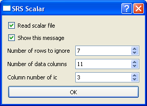
     Figure 3.13: SRS scalar dialog.

  2. Show Scalar Message (): this launches the scalar dialog (Figure 3.13). The purpose of this dialog is to control the scaling of the count rate by the storage ring current ‘ic’. This dialog contains two check boxes: the first is for choosing between scaling to ‘ic’ by reading the scalar files or not, while the second is for determining if this dialog box should appear when invoking ‘Read SRS 16.4’. The dialog also contains three integer spin boxes. The first is for the number of header rows in the scalar data files to be ignored, the second is for the number of numerical data columns in the bottom of the scalar files, and the third is for the ordinal column number of the ‘ic’ data. The ic scaling correction is based on normalising all ic’s in the tab to the ic of the first voxel (1,1) in the tab.

3.1.1.3 CCD Menu

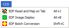
Figure 3.14: The main window CCD menu.

This menu (Figure 3.14) is for reading and processing CCD image files of EDF format. These are normal binary files with text headers. The binary data represent the CCD pixel intensity as an implicit function of the pixel position in the CCD array. The header, which occupies the first 24 lines, contains, among other things, information about the binary data type (e.g. long integer), the number of rows and columns in the CCD array, and the endian type. This information is used to read and process the data adequately. Hence, all processes are completely automated as long as the EDF file header contains the required information and has the right format. The CCD menu includes the following items

• EDF Read and Map on Tab (): to read and map a number of EDF files. A dialog first appears to enable the user to define the tab dimensions. A default directory named ‘DataEDF’ will be inspected by the program to look for EDF files if a different source directory was not selected by the user. This function can also be used for converting EDF files by mapping them first, followed by invoking ‘Write XY Data Files’ from Data menu. However, this function uses a basic EDF conversion technique (e.g. tilt and other corrections are not considered) and hence it is recommended to use multi-batch numeric conversion from MultiBatch menu.

• EDF Image Display (): the purpose of this function is to display an image of a single EDF file (Figure 3.24) and to identify the centre and radius to be used for extracting the pattern by other processes (i.e. read and map on tab, batch conversion, and multi-batch conversion). The image plotting technique is simple, that is the square of the intensity is plotted at the pixel position according to a single colour coding scheme. The purpose of using the square rather than the intensity itself is to intensify the image features. The centre of the image is indicated by an ‘$\times$’ mark. By default, the position of the centre is taken at the centre of the image rectangle and the radius is zero. By click-and-drag action, the centre will be moved to the position of click while the radius is taken as the distance between the click and the release positions. A yellow ring is plotted dynamically during the drag action. The 1D pattern will be extracted only from the part of the 2D pattern represented by the pixels inside the yellow ring. When the radius is zero the pixels of the entire image are used to generate the 1D pattern. On clicking on another position within the image, the ring centre is moved to the click position and the ring image is updated. All following batch processes that involve 1D pattern extraction will be based on the centre and radius that are identified by this function. The radius and centre data can be adjusted at any point during the session by invoking this function again and making the necessary amendments. These data will not be saved on closing the program. There are other parameters that can be adjusted within the image display dialog (see ‘EDF Numeric Conversion’ in § 3.1.1.7). Also, this dialog is launched automatically on invoking the functions that require these EDF parameters.

• EDF Batch Conversion (): this function performs batch conversion on a number of EDF files stored in a specific directory to normal images or to text files containing $xy$ data of 1D patterns. The image and text files are saved to the directory of EDF files. The program uses the default directory ‘DataEDF’ as a source for EDF files unless the user made a different choice. Three image formats are supported: png, jpg and bmp. The image and text files bear the same name as the source EDF file with proper extension, i.e. png, jpg and bmp for image files and txt for text files. A scale factor which ranges between 0.05 and 1.0 can be used to adjust the size and hence the quality of the images. By increasing this factor, the image size increases and the quality improves, with consequent increase in processing time. Based on a trial, the user should determine the scale factor as a compromise between quality on one hand and speed and size on the other, because at certain points the quality improvement may not justify the extra cost in processing time and file size. It should be remarked that jpg images require a plugin which if it is not available on the system the jpg production fails. On invoking this function a dialog (Figure 3.15) appears to enable the user to choose the image type and scale factor and to determine if ASCII text files should be written. These options are independent and hence they can be chosen in any combination including all and none. In the last case the function will terminate with no further action. If numeric conversion is selected the EDF image display dialog (Figure 3.24) will appear. In this case the program will remind the user about the image radius if the default value (i.e. 0) is used. It is noteworthy that the ASCII numeric conversion uses a basic technique and hence it is recommended to use ‘EDF Numeric Conversion’ from the MultiBatch menu, which can perform numeric conversion even on a single data set.

  

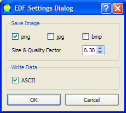
  Figure 3.15: EDF settings dialog.

3.1.1.4 Settings Menu

Figure 3.16: The main window Settings menu.

This menu (Figure 3.16) includes

• Tooltip and Cell Settings (): to launch the Settings dialog (Figure 3.17). The purpose of this dialog is to control the tooltips and grid size of the tabs. The dialog has two main sections:

  1. The first is for setting the tab tooltips. This section contains two radio buttons:

     1. Graph Tooltip: to display a graphic tooltip, that is the graph of the spectrum of the cell to which the mouse is pointing. If this option is selected, the size of the graph can be adjusted from the ‘Graph Size’ integer spin box and the associated slider.

     2. Text Tooltip: to display a text tooltip. If this option is chosen, two groups of tooltips are accessed; one for the file properties of the cell, and the other for its voxel properties. The latter include the initial properties like intensity, and the acquired properties such as statistical indicators and fitting parameters. The properties in both groups can be selected/deselected individually or as a group. Most of these properties belong to SRS 16.4 data files.

  2. The second section is for adjusting the size and aspect ratio of the tab cells. The size is modified from the ‘Cell Size Factor’ spin box and slider, while the aspect ratio is modified from the ‘X Scale Factor’ and ‘Y Scale Factor’ spin boxes and sliders. When the width of the current tab is too narrow, the tab widget handler at the top-left corner can become too small and hence the other tabs cannot be accessed. In this case, the tab width should be increased by increasing the cell size factor or the x-scale factor to gain access.

  

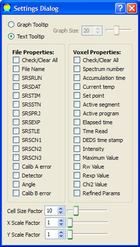
  Figure 3.17: Settings dialog.

• Grid and Colour Settings (): to launch the Tab Settings dialog (Figure 3.18) which controls the settings of tabs. This dialog contains three check boxes: ‘Grid View’ to turn the grid on/off for all tabs, ‘Single Colour’ to switch between single- and multi-colour coding schemes for all tabs, and ‘Colour Code Base’ to select a colour coding scheme that is based on a certain minimum base value chosen by the user. This base value can be adjusted from the double spin box next to this check box. When ‘Colour Code Base’ box is unchecked, the colour coding scheme will be based on the minimum of all values in the tab. It should be remarked that ‘Grid View’ and ‘Single/Multi Colour Coding’ tool buttons (see § 3.1.2.2) in the main window can be used to adjust the settings of the individual tabs independently.

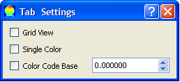
Figure 3.18: Tab settings dialog.

3.1.1.5 Fitting Menu

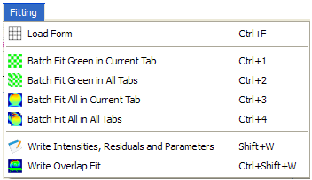
Figure 3.19: The main window Fitting menu.

This menu (Figure 3.19) facilitates curve-fitting and writing parameters. In EasyDD, curve-fitting is performed by the use of Levenberg-Marquardt algorithm which is an iterative nonlinear least-squares optimisation numerical technique. Thanks to its efficiency and good convergence, the Levenberg-Marquardt algorithm is widely used by scientists and engineers in all disciplines, and hence it became a standard for nonlinear least squares minimisation problems. The algorithm can be regarded as a combination of the Gauss-Newton method and the steepest descent method. It behaves like the former near the solution and like the latter far from it. The need for the least-squares numerical routines (including Levenberg-Marquardt) arises when a model that depends on a number of unknown parameters requires optimisation so that it best fits a given set of data according to a predefined merit function. The best fit model parameters are then obtained by varying the parameters to minimise the merit function. In the least-squares algorithms, what is required is to minimise the second norm of the residuals as given by Equation 1.5. When the parameters’ dependence is nonlinear an iterative procedure is needed where the parameters obtained from one iteration cycle are fed to the next cycle until a predefined error margin is reached or a particular number of cycles is exceeded.

In addition to the possibility of fitting all cells in a single tab or multiple tabs, it is possible to fit selected cells of a tab or tabs. With regard to batch curve-fitting, there are three ways of selecting/deselecting individual cells for batch curve-fitting:

1. ‘Ctrl’ + left mouse click to select and deselect a cell.

2. ‘Shift’ + two left mouse clicks to select a rectangular range of cells defined by the two clicked cells as diagonal corners.

3. ‘Alt’ + mouse hovering to select/deselect the cells that are hovered on.

The selected cells for fitting are marked with green colour. The keyboard ‘Esc’ button can be used to deselect the green cells.

Fitting menu contains the following items

• Load Form (): to load a spreadsheet form (see § 3.4) that defines and controls the curve-fitting process.

• Batch Fit Green in Current Tab (): to curve-fit all selected (green) cells in the current tab.

• Batch Fit Green in All Tabs (): to curve-fit all selected (green) cells in all tabs.

• Batch Fit All in Current Tab (): to curve-fit all cells in the current tab.

• Batch Fit All in All Tabs (): to curve-fit all cells in all tabs.

• Write Intensities, Residuals and Parameters (): to write the intensities, fitting routine residuals ($R_{x},R_{w},\chi^{2}$) and refined parameters of the refined cells in the current tab. Each one of these will be written to a separate file bearing a proper name (that is ‘Intensity’, ‘Rexp’, ‘Rw’, ‘Chi2’ and ‘Par$m$’ where $m$ is the parameter index). The files are saved to a directory called ‘ResParsTab$N$’ where $N$ is the current tab index. The data are structured in a 2D matrix with the same dimensions as the tab. When the fitting of the tab is partial, the non-refined cells entries will be marked with ‘NA’. It is noteworthy that the data files are formatted as in the case of using ‘Curve Fitting’ in MultiBatch menu (see § 3.1.1.7) if the check box in the multi-batch fitting dialog (Figure 3.28) is checked.

• Write Overlap Fit (): to write the refined parameters in overlapping mode. This means that the fitting data belongs to various fitting cycles with the latest cycle overwriting the refinement data only for the cells selected in the last fitting cycle without affecting the data from the previous cycles. The fitting parameters for each tab are written to a file named ‘overlapFit$N$.dat’ where $N$ stands for the tab index. The structure of this data file is similar to the structure of ‘batch’ file (see § 3.5.1). This routine is useful when applying different fitting basis functions from different forms on various parts of the same tab.

3.1.1.6 Sinograms Menu

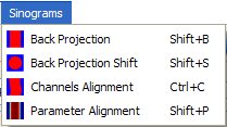
Figure 3.20: The main window Sinograms menu.

This menu (Figure 3.20) includes

• Back Projection (): to perform back projection algorithm on the current tab which represents a sinogram of rotation versus translation data. Back projection is a reconstruction technique for a 2D image from a number of 1D projections and their angles of measurement. The purpose of this algorithm, which relies on the application of the inverse Radon transform and the Fourier Slice Theorem, is to reconstruct tomographic images in real space from sinograms consisting of a set of intensity values for rotation versus translation measurements, with possible application of Fourier transform and filtering. The algorithm takes the sinogram, which is a matrix of intensities, rotates it, and sums up these values. The sinogram may require padding with zeros to a power of 2 when applying a Fourier transform. The algorithm works only when the rotational dimension is less than or equal to the translational dimension. On calling this function a dialog (Figure 3.21) will appear. In this dialog there is a ‘Fourier’ section which contains a check box to choose performing a Fourier transformation or not, and two radio buttons to choose fast (FFT) or discrete (DFT) transformation. This is followed by a ‘Data Setting’ section which includes two radio buttons to choose the sinogram type, i.e. rotation (rows) versus translation (columns) or vice versa. This is followed by an ‘Angles’ section which contains two double spin boxes to define the start and the end angles in degrees. The rotation angles are assumed to be equally spaced between these two limits with the angle step size being equal to the range (i.e. difference between the limits) divided by the number of rotations. This is followed by a ‘Read File’ check box, with a neighbouring line edit to enter the name of the angles file. This option is used when the angles are not equally spaced. In both cases the number of angles is assumed to be equal to the rotational dimension. This section is followed by a ‘Channels’ section with three radio buttons to choose one of three options: ‘Back projection for Individual Channels’, ‘Back Projection for Total Intensity’ and ‘Back Projection for Partial Intensity’. The first option performs a back projection on all common channels of all spectra in the tab individually. On performing this operation a vertical line at the position of the mouse pointer will be added to the 2D plotter (see § 3.2). On hovering the pointer over the plotter the tab will be updated to display the back-projected intensity of the current channel, i.e. the channel at the pointer position. On moving the pointer off the plotter, the tab will continue displaying the intensity of the last visited channel on the plotter. The second option will perform a back projection once on the total intensity (i.e. the sum of intensities of all channels) of the tab spectra. Similarly, the third option will perform back projection once on the partial intensity (i.e. the sum of intensities of some channels) in a certain channels range. The start and the end of the channel range are identified by the two integer spin boxes below the third radio button. Finally, there are two push buttons: ‘OK’ to proceed and ‘Cancel’ to abort the operation. The code snippet which implements the back projection algorithm is given in § A.1 in Appendix A.

  

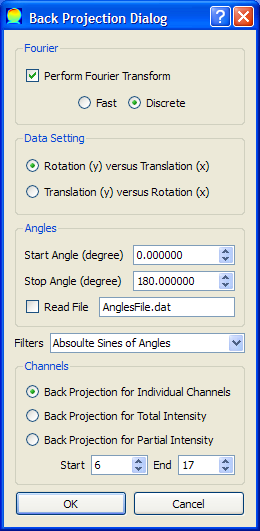
  Figure 3.21: Back projection dialog.

• Back Projection Shift (): to toggle between the normal sinogram view and back projection view for the current tab after performing the back projection in one of the three available modes.

• Channels Alignment (): to perform a sinogram alignment on individual channels of spectra. The function aligns the edge of the sample in the sinogram to a straight line using an interpolating technique that relies on a fitting parameter (usually area) of a certain peak. The fitting parameter serves as an alignment reference from which a transformation matrix for the tab rows is obtained. The technique divides the cells of each row, and assigns linearly-interpolated values to the new divisions. It then rotates these divisions clockwise and anticlockwise (i.e. displaces them left and right with move of outliers to the other side) taking in each step the sum of the square differences in the alignment parameter between the corresponding cells in the current row and the reference row. The final alignment of the row is that of the least squares. The algorithm requires applying curve-fitting on all voxels in the tab beforehand. On invoking this function a dialog (Figure 3.22) appears. This dialog contains a number of spin boxes to identify the algorithm parameters. These are: inflation factor (number of divisions of each cell), displacement number (number of divisions to be displaced left and right), parameter index (index of fitting parameter in the fitting form to be used for alignment), and upper cut-off limit (maximum value for the intensity to be set to when it exceeds that limit). The inflation factor should be between 1 and 50 inclusive. The displacement number should be between zero and a number of divisions occupying half the tab width to avoid computational waste. The purpose of the upper cut-off limit is to obtain an alignment image with sharp features. It should be remarked that this algorithm does not conserve the intensity of spectra channels as the values of the inserted divisions will be added to the intensity of the related cells. The code snippet which implements the channels alignment algorithm is presented in § A.2 in Appendix A.

  

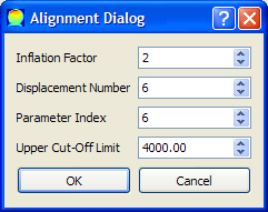
  Figure 3.22: Alignment dialog.

• Parameter Alignment (): this function is similar to the previous one but the alignment is performed on the total intensity, and the aligned intensity is displayed on the tab. This can help in testing the algorithm with a certain set of alignment parameters before applying channels alignment.

3.1.1.7 MultiBatch Menu

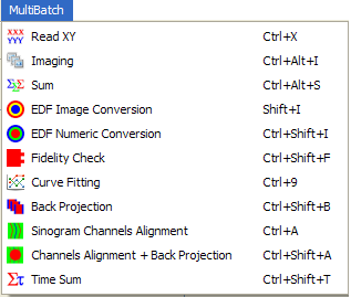
Figure 3.23: The main window MultiBatch menu.

The items in this menu (Figure 3.23) share a number of common features. First, they work on a number of data sets (including a single set) each one of which is stored in a particular directory. Second, they look to a default directory called ‘MultiBatch’ as the source of data where the data sets are stored unless the user selected another directory by using ‘Change Data Directory’ from Data menu. Third, they work on an $xy$ file format except ‘Curve Fitting’ which works on a number of formats including $xy$, and EDF functions which by nature work on EDF files. The files used by the ‘Time Sum’ function have a single user-defined name, and hence are not identified by type. Another common feature is that MultiBatch functions store the processed data either in the source directory or in its subdirectories in an organised fashion using meaningful names to facilitate managing and post-processing of results. This menu includes the following items

• Read XY (): to read a number of data sets in $xy$ format and map them on separate tabs. A maximum of 10 data sets are read in each run if the source directory contains more than 10.

• Imaging (): to produce png images representing the total intensity of spectra, similar to what the tabs display. The dimensions (rows and columns) of the images are required when invoking this function. No image will be produced for a data set if the number of data files in its directory is less than the product of the two dimensions. The image files are saved to the source directory, each with a name identical to the name of the data directory of that set with a ‘.png’ extension.

• Sum (): to produce sum spectra by adding the intensity of the corresponding channels. There is no restriction on the number of files in each data set. The number of channels in the sum spectrum is the maximum of that of the individual spectra in the data set. This function is based on the assumption that all common channels of the data set share the same $x$ coordinates. The sum files are saved to the source directory, each with a name identical to the name of the data directory of that set with ‘_Sum’ extension.

• EDF Image Conversion (): to convert EDF binary files to normal images, similar to that presented in ‘EDF Batch Conversion’ in CCD menu (see 3.1.1.3). A sample of these images is displayed (within a dialog) in Figure 3.24. The images are saved to a directory named as the data directory of that data set with an ‘_out’ extension, and stored inside this data directory. Each image is named after its EDF source file with an ‘edf’ extension replaced by a suitable extension (i.e. ‘png’, ‘jpg’ or ‘bmp’). A scale factor can also be used to adjust the size and quality of the images as explained previously.

  

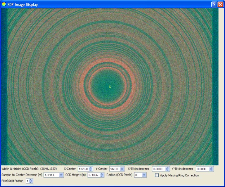
  Figure 3.24: EDF image display dialog.

• EDF Numeric Conversion (): to convert EDF binary files to ASCII numeric data files containing 1D patterns. The name of each text file is the same as its EDF parent with ‘edf’ extension replaced with ‘txt’. These files are saved to the directory of the EDF files unless a fidelity check is performed (see the next item). The function requires a number of parameters that determines the nature of conversion. Most of these parameters are defined from the EDF image display dialog (Figure 3.24) which appears on selecting a representative EDF when invoking this function. For computational efficiency, EasyDD assumes that all files processed in a single multi-batch run are obtained from the same batch, and hence have the same dimensions and the same data type (i.e. short or long integer, and big or little endian). This information (i.e. dimensions and type) is obtained from the header of the representative EDF. The user will also be offered the opportunity to run a fidelity check on the text files.

  The EDF image display dialog contains a number of widgets:

  1. Label to display the width and height of the EDF image in pixels.

  2. Two spin boxes to define the $x$ and $y$ coordinates, which correspond to the horizontal and vertical dimensions respectively, of the centre of the image rings in pixels. By default, these coordinates are set at the centre of the EDF rectangle at the start of the program. The centre is indicated on the image by a yellow ‘$\times$’ mark which moves to the new position dynamically when the coordinates are adjusted.

  3. Two spin boxes to define the $x$ and $y$ tilts in degrees within the range -89^∘ to 89^∘.

  4. Spin box for the distance in metres between the sample and the centre of the CCD detector.

  5. Spin box for the height (i.e. vertical dimension as displayed on the dialog) in metres of the CCD detector.

  6. Spin box for the radius (in pixels) of the circle that identifies the part of the EDF image to be used for numeric conversion, i.e. only the rings inside the circle will be used for extracting the pattern. The default value for the radius at the start of the program is zero meaning that the whole image will be used. A yellow ring representing the circle is displayed on the dialog when the radius is greater than zero. This ring is dynamically resized on adjusting the value of the radius from the spin box.

  7. Check box for applying the missing-rings correction based on the continuum approximation algorithm which scales the incomplete rings to the continuum value at that radius.

  8. Spin box to define a split factor for the pixels within the range 1-5. This factor was introduced because the pixel can be too coarse as a unit of length and storage due to its finite measurable size resulting in uneven distribution of intensity in the data points of the 1D pattern. The pixels of the CCD grid can therefore be split by using this factor to improve the resolution and obtain smoother patterns.

  The settings of some of these widgets are saved on exiting the program. It should be remarked that the EDF image display dialog has tooltips showing the $x$ and $y$ coordinates (in pixels) of the mouse pointer position. Moreover, the centre of the image can be moved to a new position by mouse click, and hence the yellow ring is moved and the image centre spin boxes are updated. The radius can also be adjusted by a mouse click-and-drag action, and hence the radius spin box will be updated.

  Regarding the tilt correction, a formula was derived using a standard Cartesian coordinate system in a plane perpendicular to the original beam direction that passes through the centre of the image and hence the origin of the coordinate system. For simplicity, a unit circle centred at the origin and lying in this plane was used. Here, we outline this derivation making use of the following symbols:

  $\phi$ is the angle of an arbitrary point on the unit circle ($0\leq\phi<2\pi$)

  $\theta_{x}$ is the tilt in the $x$ direction

  $\theta_{y}$ is the tilt in the $y$ direction

  $\theta$ is the actual tilt at an arbitrary point on the tilted CCD plane. It is obvious that $\theta$ is a function of $\phi$ and can have negative as well as positive values.

  

  Figure 3.25: A schematic diagram to demonstrate the derivation of tilt correction.

  From a simple geometric argument, the actual tilt as a function of $\phi$ is given by

  $$\theta(\phi)=\arctan[\cos\phi\times\tan\theta_{x}+\sin\phi\times\tan\theta_{y}]$$ (3.2)

  As can be seen, this formula retrieves the correct (and obvious) tilt in the $x$, $y$, $-x$ and $-y$ directions.

  Now referring to Figure 3.25, which is in the plane identified by the original beam and the ray directions, and on applying the cosine rule to the triangle ABC we have

  $$c=\sqrt{a^{2}+b^{2}-2ab\cos\left(\theta+\frac{\pi}{2}\right)}$$ (3.3)

  Using the sine rule we obtain the scattering angle

  $$\psi=\arcsin\left[b\times\frac{\sin(\theta+\pi/2)}{c}\right]$$ (3.4)

  And finally the required quantity, $d$, can be obtained from

  $$d=a\times\tan\psi$$ (3.5)

  It is obvious that there are other methods for finding $d$. Although this derivation is demonstrated for $\theta>0$, as seen in Figure 3.25, it is general and valid for $-\frac{\pi}{2}<\theta<\frac{\pi}{2}$.

  Concerning the missing-rings correction, because the charge-coupled device detector has a rectangular shape, the rings whose radii exceed a certain limit, by having a radius that exceeds the distance between the ring centre and one or more of the rectangle sides, will not be complete and therefore the pattern will have a reduced integrated intensity at high scattering angles. To compensate for the loss of intensity from these incomplete diffraction rings, a simple and time saving technique is used. This technique scales the incomplete rings to the continuum value at that radius by multiplying the total intensity of the incomplete rings by the ratio of the continuum circumference at that radius to the actual number of pixels in that ring. In multi-batch operations, this number is computed only once while serially reading the values of the pixels of the representative EDF file. These scale ratios are stored in a 1D vector and used during the application of the numeric conversion routine.

  

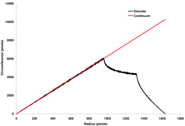
  Figure 3.26: The continuum approximation alongside the discrete value for the number of pixels in a ring.

  

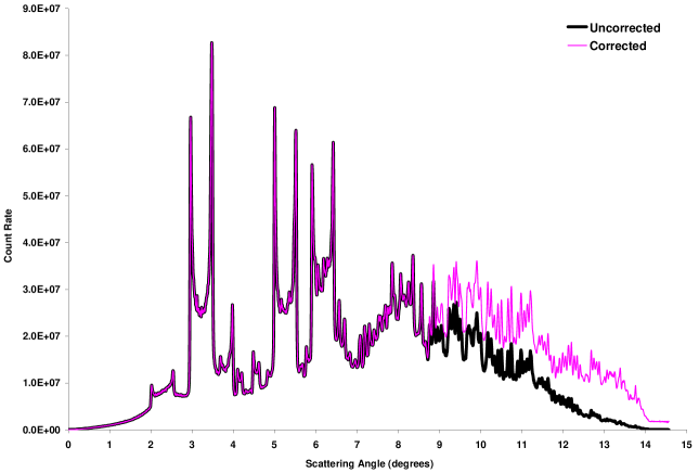
  Figure 3.27: A sample of 1D diffraction pattern extracted from a 2D EDF pattern. The pink curve is obtained with the missing-rings correction while the black is obtained without this correction.

  Figure 3.26 displays an example of the actual (discrete) number of pixels of the image rings as a function of radius in pixels alongside the continuum value of $2\pi r$ represented by the straight line. As seen, the two curves match very well for the complete rings. This indicates that the continuum is a very good approximation, except for the rings which are too close to the image corners. The meaning of the two cusps is obvious as the radius of the rings increases and exceeds the rectangle sides in one direction (i.e. vertical or horizontal) and then the other. Figure 3.27 presents a sample diffraction pattern obtained from an EDF image with and without the application of the missing-rings correction.

• Fidelity Check (): to check if some expected files, according to a guessed pattern in the naming of the data set files, are missing. These files will then be created and filled with zeros (both $x$ and $y$ coordinates) for all channels. The purpose of filling with zero is to mark these ‘void’ voxels and keep track of them as false voxels created to conserve the rectangular pattern of the slice and map it properly. The number of entries (channels) in these void files is equal to the number of points in the ordinary files (three files at the start are inspected to find the number of entries in these files and take the minimum of them if they are different). On performing the fidelity check, independently or following EDF numeric conversion, the text files are moved to a directory named after the directory of the EDF files with ‘_txt’ extension and located inside this directory. In the following we outline the fidelity check algorithm in the form of a pseudo-code:

  • Find the number of lines in a sample of three files in the data set (or all files if the data set consists of less than 4 files) and take the minimum (say $l_{min}$).

  • Obtain the name of the first file in the data set and use it as a reference string.

  • Create a flag string of 0’s with the same size as the reference string. This flag string is used to test which character position varies in the names of files.

  • Check if the names of other files have the same size as the name of the first file.

  • Check if the character at a certain position in the name of any file differs from the reference string, and set the flag position to 1 in this case.

  • Loop over all reference flag positions using a seed vector of strings (initially this vector consists of a single void string):

    • If the flag position is 1 add a character (where this character varies between the maximum and minimum found within that position in the names of files) in its position to every entry in the seed vector and hence the size of the seed vector grows.

    • If the flag position is 0 add to all strings in the seed vector the character found in the reference string in that position.

  • Test if any file is missing from the data set by comparing the list of file names to the final seed vector.

  • Create the missing files and fill them with $l_{min}$ of zero lines (i.e. lines with $x=0$ and $y=0$).

• Curve Fitting (): to perform automated curve-fitting on a large scale. The idea of this function is to deposit a number of fitting forms in the directory of the program, and store a number of folders containing data sets in the source directory. The program then performs automated curve-fitting where each pattern in every data set is fitted to each individual form and the resulting data are saved in a structured directory tree. The intensity, residuals and refined parameters files (as in ‘Write Intensities, Residuals and Parameters’ in Fitting menu) alongside ‘batch’ and ‘OlivierMatlab’ files for each data set are saved to a directory named after the fitting form and located inside the directory of that data set. A report containing information about the outcome of the fitting process is written to a file called ‘bbReport’ which is saved inside the source directory.

  On starting multi-batch curve-fitting, a dialog (Figure 3.28) appears, in which there are three radio buttons to choose the data type, i.e. ‘SRS 16.4’, ‘XY’ and ‘MCA’. The second choice requires the number of rows and columns, while the third requires this plus the number of headers and footers to be ignored. These data are input through the integer spin boxes next to the corresponding radio button. At the bottom of the dialog there are three push buttons: ‘Select Data Directory’ to identify the source directory, ‘OK’ to proceed, and ‘Cancel’ to abort the process. Next to ‘Cancel’ button there is a check box and two integer spin boxes. The check box is used to select formatting the data in the written files by fixing the width of columns and the number of decimal places to be displayed. These values are input through the adjacent spin boxes.

  

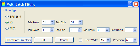
  Figure 3.28: MultiBatch curve-fitting dialog.

• Back Projection (): to perform multi-batch back projection in one of its three modes. The dimensions of the data sets and the parameters and options of back projection are determined through dialogs that appear sequentially on invoking this function. Any data set that contains insufficient number of files will be ignored. For back projecting individual channels, the resulting data files are saved to a directory having the same name as the parent directory with ‘_BP’ extension and located inside this directory. The files are named ‘BP_R$r$C$c$.txt’ where $r$ and $c$ are the row and column indices. For back projecting total or partial intensity, the resulting file of each data set is saved to the main source directory with a name identical to the name of the directory of that data set with a ‘_BP’ extension.

• Sinogram Channels Alignment (): to perform channel alignments of sinogram data in multi-batch mode. Fitting form, dimensions of slice and alignment algorithm parameters are requested on invoking this function. Data files of ‘AS_R$r$C$c$.txt’ type will be written to a directory having the same name as the parent directory with an ‘_AS’ extension and located inside this directory. A png image file of the aligned parameter, having the same name as the parent directory with ‘_fittedPeak’ extension, is also created and saved to the main source directory. Moreover, a report file called ‘saReport’ containing brief information is created and saved to the main source directory.

• Channels Alignment + Back Projection (): this is a combination of two functions: multi-batch channel alignment and multi-batch back projection. This function is provided for convenience, computational efficiency and saving disc space. The storing and naming of the resulting data files and directories follow a similar pattern to that of the parent functions. However, the prefixes and extensions are of ‘ABP’ type. A report file ‘abpReport’ is also created and saved to the main source directory.

• Time Sum (): to find the sum of a certain parameter obtained from curve-fitting for all peaks in a number of data sets as a function of the data set number. The data for each peak will be written to a *.ts type file bearing the name of the peak (usually its position value). This function assumes that the parameter data of each peak reside in a directory within the directory of the fitted data set, i.e. similar to the directory tree obtained by running multi-batch curve-fitting. At the start of this function, the user is asked to supply the common name of the files (e.g. ‘Par3’) whose data will be summed. The user will also be offered the option to normalise each sum to the maximum value within the particular sum file.

3.1.1.8 Help Menu

This menu (Figure 3.29) includes only one item:

• About (): a dialog (Figure 3.30) is launched when invoking this function. This dialog briefly defines EasyDD, offers contact information, and provides a link to access EasyDD documentation which is stored in the ‘Documentation’ directory. The latter should be a subdirectory of the program directory for normal operation.

Figure 3.29: The main window Help menu.

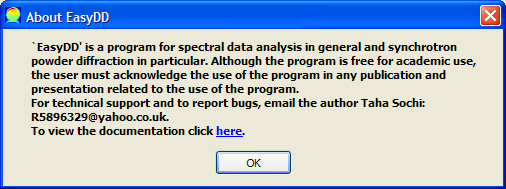
Figure 3.30: ‘About EasyDD’ dialog.

3.1.2 Tools

These include toolbars, tool buttons, spin boxes, sliders, context menus, and a status bar.

3.1.2.1 Toolbars

Most menus have associated toolbars, as seen in Figure 3.1. These toolbars can be turned on and off by right-clicking on the toolbar area and choosing from a menu. Each toolbar contains the main items of the corresponding menu. By default, all toolbars are displayed when starting the program. The selected setting will not be saved on exiting the program.

3.1.2.2 Tool Buttons

The main window contains three tool buttons (Figure 3.1):

• Grid View Button (): to turn the tab grid on/off for the current tab.

• Single/Multi Colour Coding Button (): to change the colour coding scheme between single- and multi-colour for the current tab.

• 3D Graph Button (): to plot a 3D graph of the current tab (see § 3.3).

3.1.2.3 Spin Boxes

The main window contains four spin boxes (Figure 3.1):

• Width spin box: to change the width of the tab widget window within the range 0-2000 pixels.

• Height spin box: to change the height of the tab widget window within the range 0-2000 pixels.

• Colour code spin box: to select the colour coding range scheme (see § 3.1.2.4).

• 3D Graph spin box: to scale the intensity on the $z$-axis of the 3D graph (see § 3.3).

3.1.2.4 Sliders

The main window contains two sliders (Figure 3.1). The purpose of these sliders is to adjust the minimum and maximum of the colour code range. Currently there are two available schemes which can be selected from the neighbouring integer spin box

1. ‘1’ (default) to adjust the values of the cells that fall outside the new range so that they have the value of the adjacent limit.

2. ‘2’ to eliminate these cells from the colour coding scheme and hence mark them with white.

3.1.2.5 Context Menu

The context menu (Figure 3.1) can be accessed by a right-click on the main window outside the tab widget area. This menu contains a number of items from all menus.

3.1.2.6 Status Bar

This is a standard bar (Figure 3.1) to display explanatory comments about the item that is currently hovered upon by the mouse.

3.1.2.7 Colour Bar

The colour bar (Figure 3.31) appears on reading and mapping data on tabs. The bar displays the minimum and maximum colour values of the current tab, whether the tab displays the intensity or the residuals or refined parameters after batch curve-fitting. These values are instantly updated on changing the tab selection and on moving the colour sliders to adjust the colour range. They are also updated when changing the displayed parameter by using the list widgets (see 3.1.4) following batch curve-fitting.

3.1.3 Tab Widget

This is a widget (Figure 3.1) that can accommodate a number of 2D colour-coded scalable tabs (Figure 3.31) for data mapping with graphic and text tooltips to show all essential file and voxel properties. The tabs also have a context menu with 12 items for managing rows, columns and cells in the tab. The tab widget space is a scroll area where a horizontal/vertical scroll bar emerges if the width/height of the current tab exceeds the width/height of the tab widget. On changing tab selection, the size of the tab automatically adjusts to fit the current tab.

When a tab cell is double-clicked, the 2D plotter (see § 3.2) is launched, if it is not already launched, and the pattern of the clicked cell is plotted. This cell is marked with white, but the ‘Esc’ key can be used to recover its original colour. The plotter is dynamically updated when the mouse pointer hovers over the tab so that the plotter displays the pattern of the hovered cell. By pulling the pointer outside the tab, the plotter displays the pattern of the double-clicked cell. The plotter is automatically closed when the tab widget is cleared by removing all tabs.

The tab graphic tooltip is an image of the pattern of the hovered cell while the text tooltips include its file and voxel properties, as well as the residuals and refined parameters if curve-fitting is performed. The scheme for the tab tooltips is that as long as the plotter is absent the mode of tooltips (i.e. text or graph) is determined by user choice (see § 3.1.1.4). However, when the plotter is launched the tooltips automatically become text regardless of the user choice because a graphic tooltip is redundant.

Figure 3.31: EasyDD main window following data mapping and curve-fitting.

3.1.4 List Widgets

List widgets (Figure 3.31) are created on performing batch curve-fitting on a tab, i.e. one list widget for each refined tab. These widgets contain items which include intensity, statistical indicators and fitting parameters. On selecting each one of these items, by mouse or by up or down arrow keys, the current tab colour coding and colour bar change to display the variation of the selected item.

3.2 2D Plotter

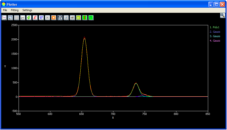
Figure 3.32: The 2D plotter.

This is a plotter (Figure 3.32) for obtaining a 2D graph of a spectrum (e.g. intensity versus energy) for any voxel in the current tab. It is also used to create basis functions and spreadsheet forms for curve-fitting. The plotter capabilities include:

• Creating, drawing, modifying and clearing fitting basis functions by simple click or by click-and-drag actions. The available basis functions are polynomials $\leq$ 6, Gauss, Lorentz and pseudo-Voigt. The last three are given in Table 1.3.

• Performing curve-fitting on the plotted pattern by a Levenberg-Marquardt nonlinear least squares algorithm.

• Saving image of the plotted pattern in 8 different formats, i.e. png, bmp, jpg, jpeg, ppm, xbm, xpm and pdf.

3.2.1 Menus

The plotter has three menus:

3.2.1.1 File Menu

This menu (Figure 3.33) contains three items:

1. Save image (): to save the plotter image in one of 8 formats.

2. Remove basis curves (): to remove the basis fitting curves and keep the refined curve.

3. Remove all curves (): to remove all curves including the refined curve.

Figure 3.33: The Plotter File menu.

3.2.1.2 Fitting Menu

This menu (Figure 3.34) contains several items and subitems:

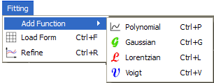
Figure 3.34: The Plotter Fitting menu.

1. Add Function: this item includes:

   1. Polynomial (): to plot a polynomial of order $\leq 6$ whose curve passes through a number of points. The points are selected by clicking on the plotting area. The order of the polynomial equals the number of points minus one. This function requires activation at the start and deactivation at the end to plot the polynomial. If the number of clicks is greater than 7 the extra points will be ignored.

   2. Gaussian (): to plot a Gaussian curve. This function requires activation at the start by selecting this item. The curve is plotted by a click-drag-release action using the left mouse button. The position is determined from the position of click, the area is determined from the rectangle of the click-release points, and the FWHM is determined from the width of the rectangle. A dynamic curve is drawn during the drag action.

   3. Lorentzian (): to draw a Lorentzian curve, as for Gaussian.

   4. Voigt (): to draw a pseudo-Voigt curve, as for Gaussian. By default, the mixing factor of the pseudo-Voigt, $m$, is 0.5.

2. Load Form (): to launch a spreadsheet for preparing or loading a form for curve-fitting.

3. Refine (): to start least squares curve-fitting by the Levenberg-Marquardt algorithm. The fitting will apply to the part of the pattern within the current $x$ range of the plotter as defined by the current view on zooming in and out.

3.2.1.3 Settings Menu

This menu (Figure 3.35) contains six items:

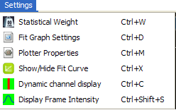
Figure 3.35: The Plotter Settings menu.

1. Statistical weight (): to launch a dialog (Figure 3.36) for choosing the statistical weight scheme in the least squares fitting. The dialog contains three radio buttons: a constant which is in the range 1-10⁹ and can be adjusted from a double spin box, a Poisson distribution with variance being equal to the observed count rate, and a reciprocal Poisson where the statistical weight equals the observed count rate.

   

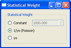
   Figure 3.36: Plotter statistical weight dialog.

2. Fit Graph Settings (): to launch the plotter settings dialog (Figure 3.37) which contains two radio buttons to choose if the fitting curve should be displayed statically on completing the refinement, or dynamically while the refinement is progressing. For the second choice a time delay (0-5000 milliseconds) for updating the curve can be set from the neighbouring integer spin box. This option is useful to monitor how the fitting converges to the solution.

   

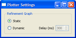
   Figure 3.37: Plotter settings dialog.

3. Plotter Properties (): to launch the plotter properties dialog (Figure 3.38) which contains three main components:

   1. Check box to show/hide plotter tooltips, which are the $x$ and $y$ coordinates of the mouse pointer position.

   2. Another check box to convert the channel number for SRS 16.4 data in the plotter tooltip to energy using a linear scaling relation. The ‘a’ and ‘b’ coefficients, which are in the range -10⁸ to 10⁸, stand for slope and intercept respectively and can be adjusted from the neighbouring double spin boxes.

   3. ‘Change Background Colour’ push button to change the plotter background colour. Three colours are available: black, white, and dark gray. The colour cyclically changes on pressing this button.

   

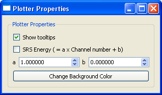
   Figure 3.38: Plotter properties dialog.

4. Show/Hide Fit Curve (): to show/hide the fitting curve following a batch curve-fitting operation when the mouse pointer hovers over the cells whose patterns have been fitted. The fitting curve will vanish when the mouse pointer leaves the tab.

5. Dynamic Channel Display (): to display the intensity of the plotter channels dynamically on the tab when hovering the mouse over the plotting area of the plotter. It should be remarked that this item is only for non-back-projected tabs. For back-projected tabs the dynamic display works in a similar way but independent of this function (see § 3.1.1.6).

6. Display Frame Intensity (): to display on tab the total intensity of the channels of the current frame of plotter when zooming in and out.

   The default of the last two functions when launching the program is to be off. Invoking these functions henceforth toggles their functionality on and off. Currently, these two functions work independently so they can be both on or off or in a mixed state.

3.2.2 Buttons

The plotter contains seventeen tool buttons; fifteen are for accessing the items of the menus and are included for user convenience. The other two, which are located on the right of the plotter, are

1. Zoom out (): this button appears on zooming in.

2. Zoom in (): this button appears on zooming out.

It is noteworthy that the $xy$ frame of the plotter is fixed on zooming in so that the displayed pattern on hovering the mouse pointer will be within the zoomed $xy$ range. The dynamic adjustment to accommodate the whole $xy$ range of the pattern will be resumed on zooming out to the initial state before zooming in.

3.2.3 Labels

Associated with each fitting basis curve is a sensitive label (coloured as its curve) on the far right margin of the plotter. On clicking the label, by left or right mouse buttons, a dialog corresponding to the basis curve is launched. From this dialog the curve parameters can be adjusted using the relevant input boxes and hence the plotter is instantly updated. The dialog also contains an image of the fitting curve equation and two push buttons: one to clear the curve and the other to close the dialog. An example of these dialogs is presented in Figure 3.39.

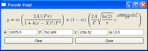
Figure 3.39: A pseudo-Voigt dialog.

3.3 3D Plotter

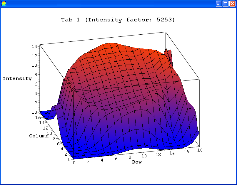
Figure 3.40: A 3D graph of total intensity as a function of voxel position in a tab.

This plotter (Figure 3.40) is used to create a 3D graph of the current tab where the $x$ and $y$ axes stand for the number of rows and columns respectively, while the $z$-axis represents the voxel intensity. The plot can be resized, zoomed in and out, and rotated in all orientations. To keep proportionality of the plot dimensions, the intensity is automatically scaled by a scale factor which is displayed beside the tab number. No more than one plotter can be launched for any tab. The plotter is closed when its tab is removed. Moreover, the label of the 3D plot is updated when the corresponding tab number changes by removing a tab. The spin box next to the 3D graph button on the main window is for scaling the $z$-axis. The range of this scale factor is between 0.1 and 100, with a step size of 0.1. On performing batch curve-fitting in one of its various modes the residuals and the refined parameters can also be visualised by the 3D plotter although the scaling may not be adequate.

3.4 Form Dialog

The main use of spreadsheet forms is in large-scale curve-fitting operations. The idea is to prepare a form within the plotter and save it to the disc. It is then imported to the main window for batch fitting a number of cells or tabs in the tab widget, or for multi-batch fitting of a number of data sets. Importing a previously prepared form to the plotter can also be used for curve-fitting a single pattern since the basis functions and frame settings, which include zoom view and $xy$ ranges, are reserved in the form. When the form dialog (Figure 3.41) is launched from the plotter, the dialog interacts with the plotter, i.e. it automatically lists the existing basis functions in the plotter. Moreover, the plotter is updated on modifying the parameters of the basis functions in the dialog.

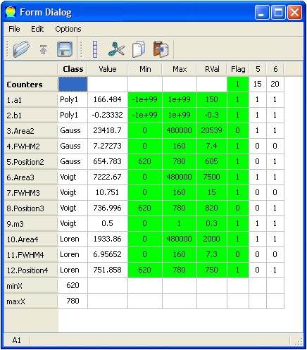
Figure 3.41: Form dialog.

The form dialog consists of a number of menus, toolbars and a status bar similar to those in the main window. The dialog also has a number of columns:

1. A gray column for labelling and classifying the parameters of basis functions. Each label starts with an ordinal index followed by the name or abbreviation of the parameter, followed by the index of the function to which the parameter belongs.

2. A column, labelled ‘Class’, in the white area for classifying the basis functions, i.e. ‘Gauss’ for Gaussian, ‘Loren’ for Lorentzian, ‘Voigt’ for pseudo-Voigt, and ‘Poly$n$’ for polynomial of order $n$. In the end of this column the $x$ range (i.e. minimum and maximum) of the form is displayed. The single, batch and multi-batch curve-fitting operations are performed only on the pattern data within this range.

3. Another column, labelled ‘Value’, for the initial values of the parameters. These initial values are automatically changed to the refined values following a single curve-fitting operation in the plotter.

4. Four green columns for restrictions. The idea of restrictions is to set the refined parameters to certain values when they exceed predefined lower or upper limits. The first of these columns ‘Min’ is for the lower limit. The second column ‘Max’ is for the upper limit. The third column ‘RVal’ is the restriction value which the parameter should be set to when it exceeds one of the two limits. The fourth column ‘Flag’ is for the Boolean flags. At the top of this column there is a global flag for the restrictions to be applied (when it is ‘1’) or not (when it is ‘0’). The other entries in the column are the individual flags for each parameter. The restriction on a certain parameter is applied only when both the global flag and the flag for that particular parameter are true (i.e. ‘1’). The default values for these four columns are shown in Table 3.1. The individual flag of a particular parameter can be set/reset (i.e. toggle between ‘0’ and ‘1’) by double-clicking the corresponding cell. Double-clicking the cell of the global flag will set/reset the whole column of individual flags. The value of the global flag can be modified by typing the value directly inside its cell. This can also be used for modifying the individual flags.

5. Column(s) for counter(s) and Boolean flags for the least squares (LS) fitting routine. These columns can be added by the user to fix the number of LS cycles and determine which parameters should be refined. Hence, these columns are absent when the form is created. On the top of each column there is a counter of positive integer type. This counter determines the number of iteration cycles in the LS routine for that set of Boolean values. Double-clicking the counter cell will set/reset the whole column of Boolean flags, i.e. they toggle between 0 and 1. The Boolean values can also be changed individually either by typing directly in the cell, or by double-clicking the cell. A ‘0’ flag means the corresponding parameter is held constant during the LS routine, while a ‘1’ flag means the parameter will be refined and adjusted in the LS routine. The default values for the counter and Boolean flags are 1 and 0, respectively. The number of cycles in the LS routine is fixed when these columns exist, and this number equals the sum of counters. When these columns are absent, the number of cycles will vary depending on the pattern, basis functions and initial values of fitting parameters. In this case, LS cycles continue until convergence is achieved within a certain marginal error. Moreover, all parameters will be refined in the LS routine.

Table 3.1: The default values of the form restrictions parameters for Gauss, Lorentz, pseudo-Voigt and polynomial basis functions. The default value for the global restriction flag is ‘0’. The ‘Plotter’ in the table refers to the frame of the plotter, as viewed by zooming in and out, when the form was created.

	Min	Max	RVal	Flag
Area	0	Plotter area	Initial value	0
FWHM	0	Plotter width	Initial value	0
Position	Plotter lower limit	Plotter upper limit	Initial value	0
$m$	0	1	Initial value	0
Poly Coefficients	$-10^{99}$	$10^{99}$	Initial value	0

3.4.1 Menus

The form dialog contains three menus: File, Edit and Options.

3.4.1.1 File Menu

This menu (Figure 3.42) contains five main items:

1. Load Form (): to load a form file to the dialog. The dialog recognises form files of *.sp type only.

2. Unload Form (): to unload a form from the dialog and erase it from memory.

3. Save (): to save a modified form to its *.sp source file.

4. Save As (): to save a form to a new *.sp file.

5. Exit (): to exit the form dialog and return to the parent widget, i.e. main window or 2D plotter.

Figure 3.42: The form dialog File menu.

This menu may also contain a number of variable items. These are the names of the most recently loaded *.sp files (up to five) made available for quick load. These items appear, when they exist, between ‘Save As’ and ‘Exit’.

3.4.1.2 Edit Menu

Figure 3.43: The form dialog Edit menu.

This menu (Figure 3.43) contains six items:

1. Add Column (): to add a column for LS counter and Boolean flags.

2. Cut (): to cut the content of selected cell(s).

3. Copy (): to copy the content of selected cell(s).

4. Paste (): to paste the cut or copied contents.

5. Delete (): to delete the content of selected cell(s).

6. Select: this item contains:

   1. Row: to select the row of the current cell.

   2. Column: to select the column of the current cell.

   3. All: to select all cells in the form.

3.4.1.3 Options Menu

This menu (Figure 3.44) contains one item:

1. Show Grid: to turn the grid on and off.

Figure 3.44: The form dialog Options menu.

The File and Edit menus have associated toolbars (Figure 3.41) which can be turned on and off by right-clicking the toolbar area and selecting the option. Each toolbar contains the main items of its menu. By default, all toolbars are displayed when starting the program, and their settings are not saved on exit. The form dialog has also a context menu which contains the items of frequent use. The context menu can be accessed by right-click on the form main area.

3.5 Modules of EasyDD

EasyDD contains four main modules; these are

3.5.1 Curve-Fitting

One of the main modules of EasyDD is curve-fitting by least squares minimisation using the Levenberg-Marquardt algorithm. Curve-fitting can be performed on a single pattern, or as a single batch process over multiple patterns, or as a multi-batch process over multiple forms and data sets. Curve-fitting can be done on single or multiple peaks using a number of profile basis functions with and without polynomial background modelling. The number of least squares cycles can be fixed or vary according to the convergence criteria. The parameters to be refined can also be selected with possible application of restrictions. The range of data to fit can be selected graphically or by using a prepared form. Some relevant statistical indicators for the fitting process, as outlined in Table 1.4, are computed in the curve-fitting routine.

Single curve-fitting is performed from the plotter on the pattern of the cell selected by a double-click. On running this mode of fitting a file called ‘aVector’ is created. This file contains a summary of the initial and final values for the fitting parameters and a number of statistical indicators. As indicated earlier, single curve-fitting applies to the $x$ range in the current view of the plotter.

Batch curve-fitting is carried out from the main window. Spectral data should be mapped on tab(s) and a form should be loaded through the main window beforehand. Batch fitting runs only on the parts of the patterns within the $x$ range of the loaded form. For successful operation, the form $x$ range should be within the $x$ range of the spectral data. Curve-fitting in this mode can be performed on a single pattern, a number of randomly selected patterns from one tab or a number of tabs. It can also be performed on all patterns in a tab or a number of tabs with no need for cell selection. Two data files are created to summarise the outcome of batch curve-fitting. The first is called ‘batch’ and contains a summary of the input and output data in general as well as data for each fitted cell. These data are labelled with ‘$t$-$r$-$c$’ where $t$, $r$ and $c$ are indices for the tab, row and column of the cell. The second file, called ‘OlivierMatlab’, is a summary intended for use in post processing. This file contains the refined parameters of the refined cells identified by ‘$t$ $r$ $c$’ labels.

Multi-batch curve-fitting is carried out from the main window. It is an automated, large-scale fitting operation on multiple data sets. The use of this mode of operation, to replace repeated manual application of batch fitting, produces more reliable and organised results and saves a huge amount of time and effort.

3.5.2 Sinogram Treatment

The main item in this module is back projection which is a tomographic technique for reconstructing a 2D image in real space from a number of 1D projections and their angles. It relies on the application of the inverse Radon transform and the Fourier Slice Theorem. The raw data for back projection are sinograms consisting of a set of intensity values for rotation versus translation measurements. Back projection can run in single and multi-batch modes, and can be applied on total or partial intensity as well as individual channels, with possible application of Fourier transform and filtering.

3.5.3 EDF Processing

The purpose of this module is to extract the information from EDF binary files obtained from CCD detectors. Two forms of extraction are available: conversion to normal 2D images in one of three formats (png, jpg and bmp), and squeezing to 1D patterns in $xy$ text format.

3.5.4 Graphic Presentation

Examples of this module are mapping, visualisation and imaging to produce graphs in 2D and 3D spaces. These include creating tomographic and surface images in single, batch and multi-batch modes, as well as $xy$ plots for spectral patterns. Some of these graphic techniques use a direct display on the computer monitor, while others save the results to the computer storage in the form of image files.

3.6 Context Menus

EasyDD contains several context menus which are accessed via right-click:

• Main window context menu: contains selected items from the main window menus.

• Main window toolbars context menu: used to turn the main window toolbars on and off.

• Tab context menu: contains 12 items for manipulating cells, rows and columns of the active tab.

• Form dialog context menu: contains selected items from the form menus.

• Form dialog toolbars context menu: used to turn the form toolbars on and off.

Chapter 4 Tomographic Studying of Heterogeneous Catalysis

In this chapter we outline the experimental part of our investigation which focuses on the study of tomographic imaging of heterogeneous catalysis.

4.1 Catalysis

A ‘Catalyst’ is a chemical agent that affects a chemical reaction by increasing or decreasing its rate. ‘Catalysis’ is the involvement of catalysts in chemical reactions. Catalysts can be in any one of the three phases (i.e. gas, liquid and solid) although most industrial catalysts are solids or liquids. Important catalytic characteristics that determine their suitability for use in a given process include activity, selectivity, cost and lifetime. By controlling the rate of chemical reactions, catalysts can play a vital role in the production of important chemicals under manageable conditions. Another property of catalysts which can be more important than activity is their ability to affect the selectivity of reactions where different products can be obtained from given reactants by the choice of catalytic system. Reaction routes can be designed with the help of catalysts to maximise useful products and reduce waste and cost [29].

The intentional use of catalysts in industrial projects started in the mid 18th century with the use of lead chambers in the production of sulphuric acid. Since then, the use of catalysts in the chemical industry has become a necessity in most manufacturing processes. Very important industrial and fine chemicals are produced with the help of catalysts. It is estimated that 75-90% of all synthetic chemicals are produced using catalysts. Examples of chemicals that require catalysts in their production include pharmaceuticals, resins and synthetic fibres. The petrochemical industry heavily relies on the use of catalysts in refining, purification and chemical transformation processes. Catalysts have also very important uses in environmental protection technology such as emission control. Although catalysts have been in use for a very long time, the theoretical basis for their action had not been established until the last few decades. Indeed, the use of catalysts in many areas is still an art rather than a science [62].

Although catalysts do not change the thermodynamics of reaction, they can lower the transformation activation barrier by introducing a new pathway for a reaction. Despite the widespread belief that catalysts are not affected in the course of reaction, they in fact participate in a cyclic process of chemical bonding with the reactants. While catalysts in general are not consumed in reactions, they may require replenishment to compensate the losses which occur by associated processes. They may also undergo chemical changes that reduce their activity. Different deactivation mechanisms are responsible for the progressive loss of activity [29].

According to their production method and structure, catalysts can be divided into three groups: bulk, shell and impregnated. Industrially used catalysts come in various shapes and forms such as spheres, cylinders, pellets and rings. Sophisticated manufacturing processes which involve physical and chemical treatment under strictly-controlled conditions are followed in the production of these catalysts. The purpose is to produce these agents with the required properties as demanded by the intended process [121].

4.2 Heterogeneous Catalysts

Catalysts can be either homogeneous or heterogeneous. In homogeneous catalysis the reactants and the catalyst are in the same phase, while in heterogeneous catalysis they have different phases such as gas and solid. A typical case of Heterogeneous catalysts is in the use of a solid support that contains traces of active catalytic metal such as molybdenum or nickel particles. They facilitate the reaction by allowing the reactants to diffuse and adsorb onto the surface, coming in contact with the catalyst. The products then desorb and diffuse away on completing the reaction. The rate of reaction is determined by the speed of transportation of reactants and products in this bidirectional process. Highly porous materials with high internal surface area, such as alumina, zeolites and silica, are therefore favoured for use as catalysts and catalytic supports. The surface properties of these agents are very important when selecting a catalyst for a particular process [21].

Heterogeneous catalysts have very important scientific, environmental and technological applications. They are widely used in various organic and inorganic industries such as oil refinement, bio-fuel production, hydrocarbon cracking, fat hardening, environmental protection and fine chemicals synthesis. One of the main advantages of using heterogeneous catalysis is the ease of separation from the reactants. This partly explains the exclusive use of these functional materials in most industrial catalytic processes over homogeneous catalysis. Another advantage is that they can be maintained at higher temperatures than the homogeneous catalysts. Various properties are considered in the use of heterogeneous catalysts; these include chemical and mechanical stability, porosity, high internal surface area, ease of handling, separation, safety and cost [121].

Metal oxides play a vital role in many industrial heterogeneous catalytic processes. Molybdenum is widely used as a catalyst in many industrial applications. This is partly due to its diverse oxidation and reactivity states. Nickel is one of the most catalytically active metals and hence is widely used in various industrial processes. Its applications include desulphurisation of organic compounds, hydrogenation and hydrogenolysis. Molybdenum, nickel and cobalt on $\gamma$-alumina supports are commonly used in industrial hydro-treatment processes [130, 134].

Alumina is commonly used as a heterogeneous catalyst and as a support for a large number of industrial catalysts; in fact it is the most widely used catalytic support. As an example, alumina is widely used in environmental protection technology. Alumina is either extracted from natural mineral deposits or synthesised from aluminium hydroxide and oxide. It is stable at high temperatures with excellent mechanical and thermal properties. It also has a large internal surface area per unit volume thanks to its highly porous structure (see § 4.2.1 for some typical values). This surface area can be used to support tiny particles of active materials. Alumina supports are produced by thermally dehydrating Al(OH)₃ or AlOOH. Alumina exists in a crystalline $\alpha$ form and other transitional forms such as $\beta$ and $\gamma$. The crystalline form is not usually used as a catalytic support due to its low surface area [29].

Extrudates are a form of catalyst support material, shaped as cylinders and manufactured by forcing a mass to flow through a hole using high pressure. Extrudates are generally used for impregnated catalysts. Typical sizes of extrudates used in the catalysis industry are 10-30 mm in length with 1-5 mm in diameter. Important issues to be considered when using extrudates in catalysis are porosity, ease of manufacturing, cost, mechanical strength and ability to survive the reaction conditions [29].

The optimal distribution of active sites in supported catalysts is dependent on the type and speed of the required chemical reaction. For slow reactions where the speed of transportation is not a limiting factor, it is desirable to have a uniform distribution to maximise the distribution of active sites and hence catalytic exposure. For reactions involving heterogeneous catalysis where diffusion plays a crucial role in determining the reaction rate, it is beneficial to deposit the active catalytic sites near the surface of the catalytic support body. Hence an egg-shell distribution is desirable in this case. Egg-shell distribution is also advantageous in the case of consecutive reactions with unwanted secondary products to maximise selectivity of primary products. Heat transport mechanisms also impose limitations on the distribution of active sites on considering the nature of the catalytic reaction as an endothermic or exothermic. Egg-white or egg-yolk distributions are preferred when the reactants are contaminated with a catalytic poison [84, 102].

Catalyst impregnation is one of the most important techniques for catalyst support preparation. The technique is widely used thanks to its low cost and simplicity. The impregnation methods are generally divided into pore volume impregnation and wet impregnation. In the first case the infused solution volume is comparable to the pore volume and the distribution of the active ingredients is determined by capillary forces. In the second case the volume of solution considerably exceeds the pore volume and the distribution is influenced by diffusion and adsorption forces. A required distribution profile of active sites can be engineered by controlling impregnation parameters such as pH, temperature, concentration of solution, impregnation time, drying conditions, choice of precursor, and so on [91, 56, 107, 92, 93].

In the rest of this thesis, we present some examples of using EasyDD in processing and analysing powder diffraction data obtained from synchrotron radiation facilities in the context of heterogeneous catalysis investigations. In fact large parts of EasyDD were specifically developed to facilitate processing, analysing and visualising of these massive data sets. The examples are ordered chronologically to reflect the evolution of the use of X-ray tomographic techniques for the investigation of metal oxides anchored to alumina supports. In most cases, the role of the author of this thesis has been in data collection, data processing and analysis. In the earlier short two sections, 4.2.1 and 4.2.2, the main intellectual ownership of the results lies with the cited authors and the main contribution of this author was to help the data analysis and develop specific aspects of the software to do that; in the latter section, 4.2.3, the author is the main contributor to the given results. In respect of the various results outlined in this thesis, the role of the author will be highlighted as necessary.

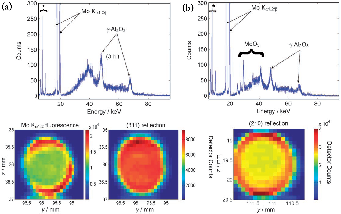
Figure 4.1: Detector signal from a Mo/Al₂O₃ catalyst body (a) after drying at 120^∘C and (b) after calcination at 500^∘C (after Beale et al [17]).

4.2.1 2D TEDDI Study of Distribution of Precursors and Active Catalysts

This investigation was carried out by Beale et al [17]. The samples used in this study are cylindrical objects of alumina (Al₂O₃) as a base impregnated with active metallic catalysts. Here, we quote Beale et al for the description of the samples: “The cylindrical $\gamma$-Al₂O₃ extrudates possessed a diameter of 1.5 mm, a length of 10 mm, a pore volume of 0.86 mLg^-1, and a surface area of 245 m²g^-1. The Mo/Al₂O₃ sample was prepared using pore-volume impregnation with a 1.8M Mo(NH₄)₆Mo₇O₂₄.4H₂O solution at pH 6.0. Drying was started 1 h after impregnation by passing hot air over the sample until the temperature reached 120^∘C. The Co–Mo/Al₂O₃ sample was prepared using a 1.0M Mo(NH₄)₆Mo₇O₂₄.4H₂O and 0.6M Co(NO₃)₂ solution at pH 5.0. This sample was allowed to age for 15 min before drying. Subsequently, both samples were calcined at 500^∘C for 1 h in static air.”

The measurements were carried out at station 16.4 of the Daresbury Synchrotron Radiation Source. This station operates with three coupled MCA detectors and uses a multi-chromatic beam to gather data in EDD mode. The use of a white beam also allows for the detection of fluorescence signals. In this investigation, TEDDI was used to collect information about phase and elemental distributions on supported metal oxides in catalyst bodies during different stages of catalyst preparation. The distribution of the active catalyst (i.e. molybdenum trioxide MoO₃), as a crystalline phase present only in the post-calcined sample, was determined from the diffraction signal, while the distribution of the precursor (amorphous) phase in the pre-calcined sample was determined from the Mo/Co fluorescence signal. Some of the results which have been obtained from this investigation are presented in Figure 4.1. EasyDD was used in the visualisation and analysis of the data collected in these measurements. The images were reconstructed directly after beam and count rate corrections with some of these corrections being implemented in EasyDD.

This study highlighted the potential of TEDDI to acquire 3D information about the elemental and phase distributions of metal oxides embedded in catalytic supports. The stages of catalyst formation from the precursor phase was partly displayed. It also highlighted the prospects of using TEDDI with in situ and dynamic phase transformation studies. The results of this study emphasised the advantage of EDD as a viable data acquisition technique with the benefit of utilising fluorescence signals which contain extra information about the phases involved in the reactions. It is noteworthy that the two peaks, seen in Figure 4.1, at $E\simeq$ 24.9 and 27.4 keV, which were not identified previously, can now be identified as the ($hkl$, $d$ Å) = (004, 2.2759) and (241, 2.0671) Bragg reflections of aluminium molybdate.

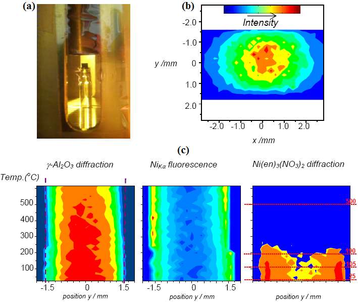
Figure 4.2: (a) 3 mm extrudate mounted in an environmental cell and (b) signal distribution (2D slice) through a supported catalyst are shown. In (c) the signals from a spatial 1D time/temperature scan, depicted as a 1D map, are shown in which both diffraction (from alumina and precursor) and fluorescence (from nickel) signals are collected at each point.

4.2.2 2D Spatial/Temporal TEDDI of Alumina Supported Catalyst Bodies Under Preparation

This investigation was carried out by Espinosa-Alonso and coworkers, and the results are published in [49]. The main objective was to examine the calcination of a heterogeneous catalyst, and monitor the genesis of active phase formation during the heat treatment. The sample used in this study is similar to the one used in the previous example. However, nickel on alumina was used and the initial precursor Ni(en)₃(NO₃)₂ decomposes at about 190^∘C to leave a supported Ni/$\gamma$-Al₂O₃ catalyst with an egg yolk distribution. Again TEDDI was used in this investigation but this time in both spatial and temporal mode. The author participated in the data collection of this experiment. Moreover, EasyDD was used in processing, visualising and analysing of these data. A sample of the results is graphically presented in Figure 4.2.

This study demonstrated the suitability of TEDDI for probing temporal dimensions as well as spatial dimensions. However, the technique is relatively simple compared to the CAT type ADD experiments (next example). The reason is that each time frame contains only 1D spatial sample (row) information. Again, fluorescence signals, as well as diffraction signals, were exploited to gain information about polycrystalline phase and elemental distributions in the sample, and this feature is typical of the energy dispersive mode. The study revealed that the spatial and temporal distributions of the precursor and active catalyst are subject to considerable variation. This indicates the sensitivity and delicacy of the formation process, and its dependency on the fine details of preparation and thermal treatment procedure.

4.2.3 3D Spatial/Temporal CAT Type ADD Studies of Alumina Supported Catalyst Bodies

In the previous study (§ 4.2.2) 2D spatial tomography with a crude temporal aspect was achieved. In the current study the aim was to have increased temporal resolution, while maintaining similar spatial resolution, in order to investigate the formation of an active extrudate-supported MoO₃ catalyst under calcination. In this experiment CAT type ADD (see § 1.3.4) was employed to look at the temporal and thermal behaviour of a slice through an extrudate sample undergoing calcination to obtain 2D data at various points in time. The temporal aspect to the study makes it entirely novel and challenging, requiring the data acquisition to be sufficiently fast to make the process observable. The pertinent information is collected by making individual diffraction collections from the sample at different positions and different orientations, as presented in Figure 4.3.

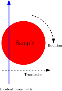
Figure 4.3: CAT configuration used in the 3D spatial/temporal CAT Type ADD experiment.

At the time of data collection, CAT type angle dispersive methods had only very recently been demonstrated in the literature [20]. Proportional area detectors, such as CCD and CMOS-based devices, can be used for recording angle dispersive diffraction patterns, and hence can support much higher count rates than energy dispersive solid state detectors. Since these modern devices offer fast reading, they can provide a more thorough insight into the temporal dimension of the dynamic processes under investigation. The area aspect of such detectors allows the recording of entire powder rings in angle dispersive mode, which can be integrated to give 1D powder patterns with good signal-to-noise ratio. The recorded intensity would be severely reduced if only a strip detector was employed. Such area detectors, when used in conjunction with very bright sources, allow for very fast data acquisition even from materials that give fairly poor scattering.

By contrast, the current technology of EDD detectors does not support high count rates. Moreover, area type EDD detectors are not realistically available and hence EDD collection is normally limited to a small solid angle of space. Although the number of photons in a white beam is considerably higher, the benefits of high intensity cannot be fully exploited due to the limitation on the count rate of EDD detectors. The CAT type geometry, with the associated algorithms, offer a convenient method for recording and reconstructing a whole slice through the sample in a short period of time. Traditionally, CAT is used in medical physics for looking at variations in object attenuation (e.g. CAT scans in hospitals) and the study of objects by micro-tomography. The view was that this method could be equally applied in the investigation of supported catalyst bodies to produce valuable new information on the formation processes.

In this experiment an uncalcined Mo-loaded extrudate, taken from the same batch of the experiment described in § 4.2.1, was used. This system was chosen for a number of reasons

1. The already existing data from previous experiments showed the expected distribution of the active phase. This acts as a check on the distribution of the reconstructed images produced from the CAT type experiment.

2. The amount of formed active catalyst is expected to be relatively high such that one can reasonably expect to be able to observe active catalyst concentrations within the diffraction patterns.

3. The temporal evolution is unknown, so it was concluded that this experiment would yield new useful information about this system.

4. The experiment would collectively lead to a proof-of-concept study while also revealing useful information on a real process.

The sample is mounted, with its longitudinal axis vertical, on a mounting pole which is then attached to a goniometer, as seen photographically in Figure 4.4 (a) and schematically in Figure 4.4 (b). The goniometer, which serves to align the sample, is mounted on a rotation stage, which is itself mounted on a translational stage, with the horizontal translation being perpendicular to the beam direction. The sample is heated by a hot air blower which is mounted on the translation stage such that during translation the alumina extrudate and the heater move together, yet the extrudate is free to rotate. During the recording of one slice, and for the purpose of rapid data acquisition, the sample is continuously translated through -1.5 to +1.5 mm with respect to the centre of the extrudate. During this process diffraction is recorded on a fast area detector in approximately 0.1 mm steps, thereby equating to a total of 31 translation measurements. This is being done at orientations from 0^∘ to 180^∘ in steps of 6^∘, and hence the rotation measurements are also 31 in number. The total number of measurements for each slice is therefore 961. Each measurement is contained in a binary EDF file (see § 3.1.1.3). The acquisition time of about 0.5 second per measurement with the associated motor movement time gives an overall collection time of approximately 10 minutes to record a slice represented by a single data set. It is important to note that diffraction occurs along the entire length of the beam-sample interaction and this causes an intrinsic spread in recorded angle. This effect is worst at the longest path lengths near the centre of the extrudate. The use of high energy X-rays mitigates this, since the reflections occur at lower scattering angles.

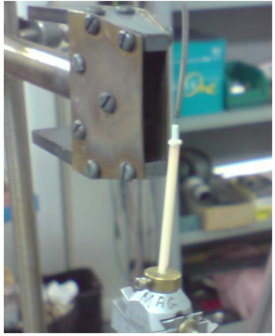
Figure 4.4: (a) Photograph and (b) schematic illustration of the mounted extrudate sample system.

Figure 4.5 is a sample sinogram displaying the integrated intensity of the largest alumina peak, and hence contains information on the distribution of alumina in the extrudate. It clearly shows the diameter of the alumina cylinder which can be estimated to be about 1.7 mm. The image also highlights the nature of information conveyed by a sinogram.

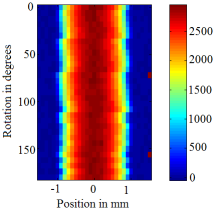
Figure 4.5: A sinogram representing the integrated intensity of the largest alumina peak at $2\theta=5.77^{\circ}$. The peak profile is modelled by a Gaussian.

Table 4.1: List of time and temperature stamps for the 22 data sets of molybdenum experiment. The time is given in minutes while the temperature is in ^∘C.

Index	Data set	Time	Temperature	Index	Data set	Time	Temperature
1	ambient	0	25	12	ramp11	110	575
2	ramp1	10	75	13	ramp12	120	625
3	ramp2	20	125	14	ramp13	130	675
4	ramp3	30	175	15	final0	140	700
5	ramp4	40	225	16	final1	150	700
6	ramp5	50	275	17	final2	160	700
7	ramp6	60	325	18	final3	170	700
8	ramp7	70	375	19	final4	180	700
9	ramp8	80	425	20	final5	190	700
10	ramp9	90	475	21	final6	200	700
11	ramp10	100	525	22	final7	210	700

There are 22 data sets: 1 at ambient temperature, 13 at ramp-increasing temperatures, and 8 at a steady-state final temperature. These sets, which are all collected from a single circular slice from the cylindrical sample, represent the dynamic state of the sample as a function of time and temperature. The time and temperature stamps of these data sets are presented in Table 4.1. As each set consists of 961 files, the total number of files is 21142. The size of each EDF file is about 9.5 megabytes, and hence the total size of the EDF files is about 200 gigabytes. In a few cases data files for some voxels were missing, and hence void files were inserted in their positions to maintain the voxels positions when mapping and visualising the slices. These data sets are shown in Figure 4.6. The images display the total intensity (sum of counts of individual voxels in each data set) of the 22 sinograms (which represent rotation on $y$-axis in degrees versus position on $x$-axis in millimetres).

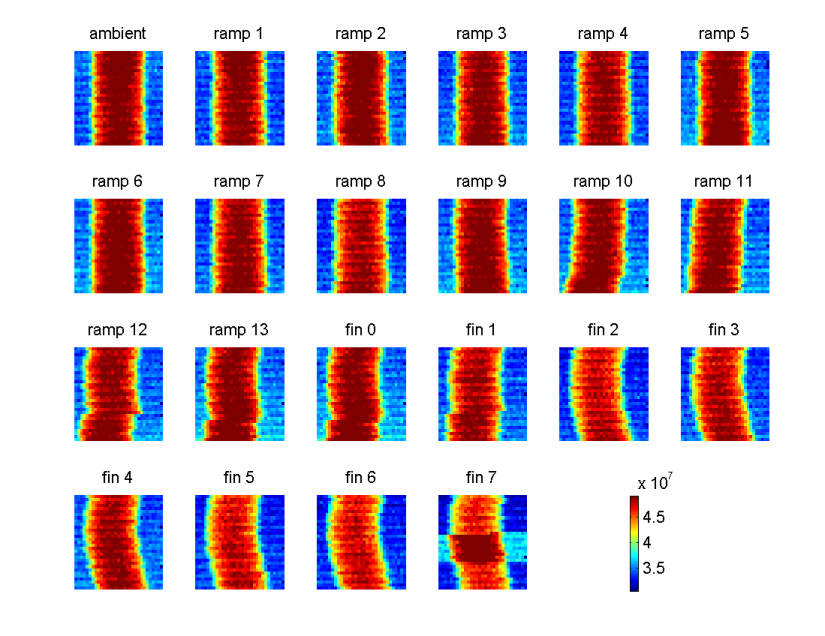
Figure 4.6: The 22 data sets of molybdenum experiment displayed as total intensity sinograms.

The experimental setting and data collection were performed by S. Jacques and coworkers, while data processing, analysis and visualisation were carried out by the author and S. Jacques. EasyDD was the main tool used in the analysis of these data. The measurements were performed at the European Synchrotron Radiation Facility (ESRF) beamline ID15B which is dedicated to applications using very high energy X-ray radiation. ID15B houses the angle dispersive diffraction setup using a large area detector [50]. The monochromatic beam used in this experiment has a wavelength of 0.14110 Å.

In the following we outline the data processing stage and present results obtained from analysing these data sets. First, to ensure the consistency of data collection mechanism, the time stamps of the individual files for each data set were gathered and compared to the device time stamp which is archived in an independent log file. The comparison revealed that the timing is consistent with no apparent error. The time stamp also provided a graphical picture of the time-temperature correlation.

As the original data are in the form of binary EDF images, they have to be converted to 1D patterns in ASCII numeric format. Datasqueeze (see § 2.13) was used to perform this conversion because at that time the EDF processing module of EasyDD had not been implemented. The squeezing process (which took about a week to complete on a fast dual-processor pentium workstation) was repeated three times to ensure consistency and accuracy of the results and eliminate errors. Each extracted text file contains three columns of data: scattering angle in degrees, number of counts computed by integrating around the entire ring, and an error index.

When constructing the sinograms from the individual slice measurements, it became apparent that there was a misalignment problem, mild in some data sets and severe in others. The problem is obviously due to a mechanical error in the translation/rotation system. This resulted in a ragged edge of the sample voxels in the sinograms, as seen in Figure 4.6. To correct this error, a large alumina peak was used to calibrate the positions of the peaks (see Channels Alignment in § 3.1.1.6). By correctly aligning the sinogram voxels with respect to the alumina peak, a transformation matrix T for each data set was obtained. These matrices were then applied to all channels of the diffraction patterns of their respective data sets to correct the sinograms and align the other peaks. This operation is graphically presented in Figure 4.7. Also, a sample sinogram before and after alignment is shown in Figure 4.8.

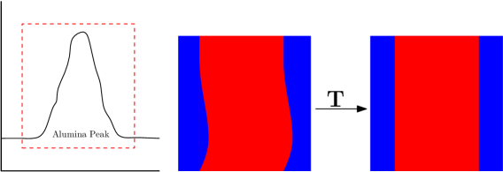
Figure 4.7: Sinogram alignment using a prominent alumina peak. The alignment matrix T obtained from this operation is used to align the sinogram channels. In these schematic sinograms, blue represents the background while red represents the sample voxels.

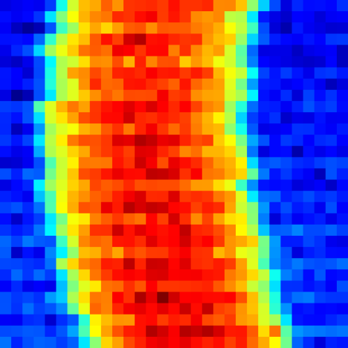
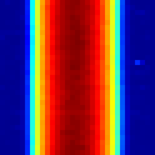
Figure 4.8: An example of a sinogram (a) before and (b) after alignment.

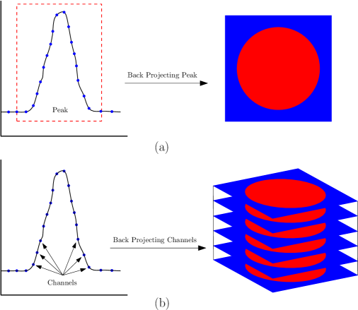
Figure 4.9: Back projection (a) of a diffraction peak and (b) of a number of channels in a diffraction peak. In these schematics blue represents the background while red represents the sample voxels.

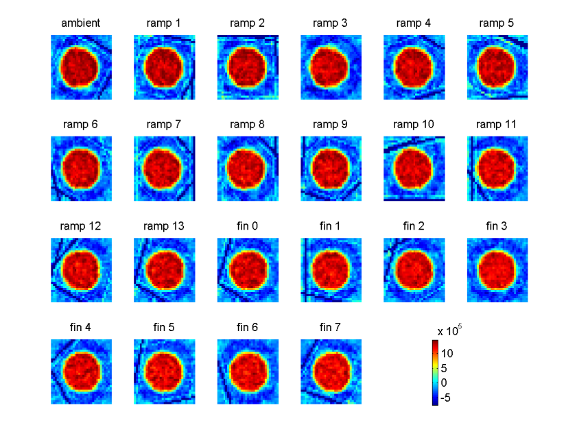
Figure 4.10: The 22 data sets of molybdenum experiment displayed as total intensity of reconstructed images.

Following this alignment correction procedure, back projection (see § 3.1.1.6 and § 3.5.2) was used to convert the sinograms to normal 2D spatial images of slices. In this regard, there are two ways of applying back projection. The first is to apply it to a collective feature such as the intensity of a given pattern or peak, while the second is to apply it to all the individual channels. These two approaches are demonstrated schematically in Figure 4.9. Back projection of individual channels was chosen for our reconstruction procedure. Figure 4.10 shows the total intensity (i.e. sum of all channels) of the reconstructed images which represent the local positions of the voxels in the 2D slices in real space.

In Figure 4.11 the sums of diffraction spectra from these data are displayed. The 22 curves in bottom-up order correspond to the 22 data sets in their temperature and temporal order. This figure summarises the information contained in each set. The sums are also presented in Figure 4.12 as a stack plot in a 3D graph.

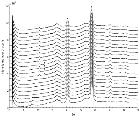
Figure 4.11: Sums of back-projected diffraction patterns of the 22 data sets of molybdenum experiment presented as a stack of plots in a 2D graph.

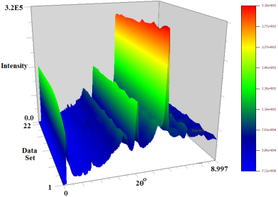
Figure 4.12: Sums of back-projected diffraction patterns of the 22 data sets of molybdenum experiment presented as a stack of plots in a 3D graph.

Following back projection, and guided by the stack plots, EasyDD was used in multi-batch processing mode with restrictions to curve-fit the diffraction peaks. First, a large number of peaks (about 70) were chosen for fitting. These represent the prominent and the suspected peaks from all 22 stages. The purpose of this approach is to capture and curve-fit all important peaks although some of them are repetitive. As the peak may be more prominent in one stage than in another, and since peak position may change with temperature, the use of various temperature stages for peak selection is intended to ensure that all peaks of interest are captured at their ideal state and position. We also systematically inspected the 2D stack plot to ensure that all the peaks in the sum plots are included. Most peaks were fitted individually and some were fitted as couples. In all cases, a simple Gaussian profile was used to model the peak shape while a linear polynomial was used to model the background. It should be remarked that this whole operation has been completed in less than a day (few hours of manual work to prepare forms and few hours of computer processing using EasyDD). This stands in sharp contrast to the required time and effort (estimated to be many months of hard labour) to perform such a task manually using conventional tools.

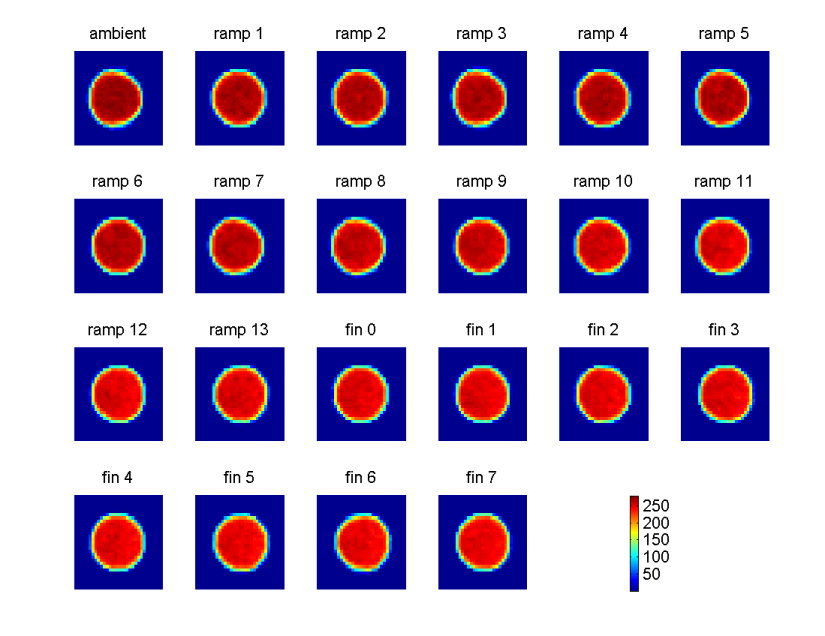
Figure 4.13: Integrated intensity of the largest alumina peak at $2\theta=5.77^{\circ}$ modelled by a Gaussian profile.

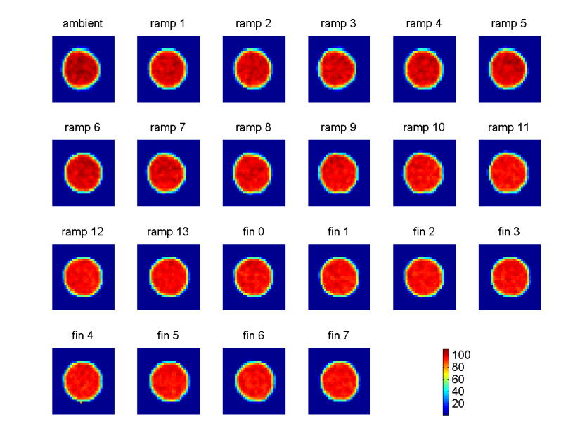
Figure 4.14: Integrated intensity of the second largest alumina peak at $2\theta=4.05^{\circ}$ modelled by a Gaussian profile.

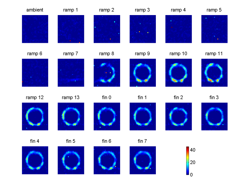
Figure 4.15: Integrated intensity of a molybdenum compound peak which is the Bragg reflection at $2\theta=2.10^{\circ}$ modelled by a Gaussian profile.

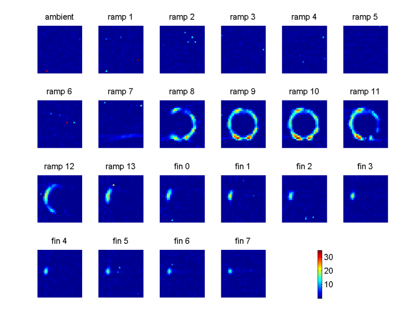
Figure 4.16: Integrated intensity of another peak of a molybdenum compound which is the Bragg reflection at $2\theta=2.50^{\circ}$ modelled by a Gaussian profile.

Figures 4.13, 4.14, 4.15, and 4.16 present some of the results obtained from this analysis. Each figure contains 22 colour coded tomographic images (corresponding to the 22 data sets) of spatial distribution of phases. The displayed parameter in these colour coded images is the integrated intensity (i.e. Gaussian area) of these peaks. These figures display 4 prominent peaks (2 for alumina and 2 for molybdenum compounds) in the spectra of these data sets. These 4 peaks are also presented graphically in plots of intensity versus scattering angle in Figures 4.17, and 4.18. In each one of the tomographic figures the data sets are labelled according to the temperature stage, that is ambient, ramp and final (abbreviated by ‘fin’) which represents a final stage where the temperature reached a constant steady-state value. Various distinct crystallographic entities with different distributions can be seen to form during the calcination process. The molybdenum compound images (Figures 4.15 and 4.16) reveal that the phases are distributed unevenly and only on one side of the sample at some stages. The distribution of molybdenum compound phases is consistent with an egg-shell configuration.

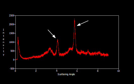
Figure 4.17: The most prominent alumina peaks in a plot of intensity (in number of counts) versus scattering angle (in degrees).

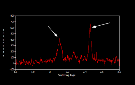
Figure 4.18: The most prominent peaks of molybdenum compounds in a plot of intensity (in number of counts) versus scattering angle (in degrees).

In Figure 4.19 the disappearance of a precursor phase during calcination is shown. Figure 4.20, which pertains to the largest alumina peak, demonstrates the observed position shift in the peaks due to temperature change. The parameter displayed in this figure is the position of the Gaussian fitted peak. This figure shows maps of the peak centre of the fitted alumina peak as a function of data set and hence temperature. From the colour bar, it can be seen that the peak centre is moving towards lower scattering angle as the temperature increases. This obviously corresponds to an increase in the $d$-spacing, consistent with unit cell expansion that is expected with increasing temperature. In this figure the background is masked and the colour code range is narrowed to accentuate the position shift feature. The figure also reveals a thermal gradient across the sample (increasing from left to right) which is due to uneven heating because of positioning of the heating element on one side of the sample.

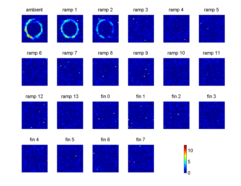
Figure 4.19: Disappearance of precursor during calcination as demonstrated by the Gaussian integrated intensity of the peak at $2\theta=0.771782^{\circ}$.

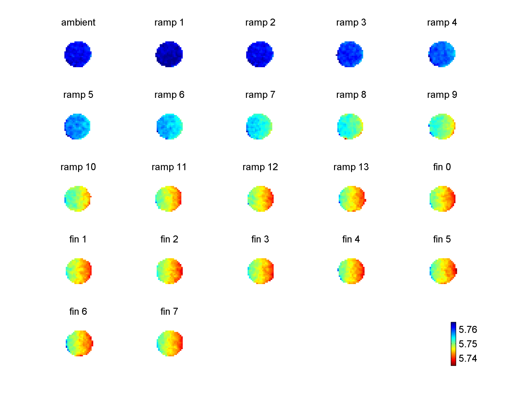
Figure 4.20: Change of position of the largest alumina peak at $2\theta=5.77^{\circ}$ with increasing temperature. The stability in the last stages indicates a steady-state.

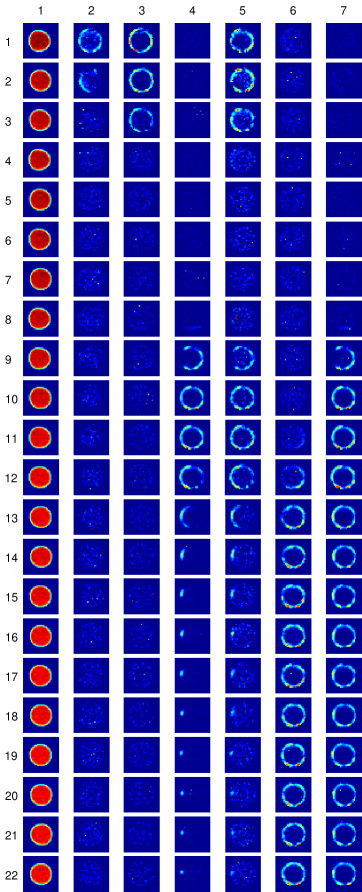
Figure 4.21: Phase distribution patterns of molybdenum data. The rows and columns are labelled with their indices and the background is masked.

To investigate the phases that exist in the molybdenum experiment sample systematically, we produced Phase Distribution Patterns (PDP), seen as columns in Figure 4.21. The idea of PDPs is to classify the phases in their spatial distribution in the slices as presented in the 2D colour-coded tomographic images. The general assumption is that each PDP is a finger print of a single crystallographic entity, although this assumption may not be valid in general as some phases may be present in more than one PDP. By inspecting the PDPs and comparing them to the peak positions in the stack plots, the phases can be identified if standard diffraction pattern data, such as those obtained from Inorganic Crystal Structure Database (ICSD) [77], are available.

Several phase distribution patterns are observed in the molybdenum data sets; the main ones are presented in Figure 4.21. The tomographic images in this figure are obtained from mapping the integrated intensity of the peaks. Each PDP was observed from a number of peaks with specific scattering angles. In the following we discuss these phase distribution patterns, as represented by the columns of Figure 4.21 from left-to-right order, trying to link them to specific crystallographic phases. In all cases, we used standard diffraction patterns obtained from the ICSD database in phase identification:

1. The first PDP (first column from left) obviously comes from alumina. The following peaks of $\gamma$-alumina [106] were identified with this PDP: ($2\theta^{\circ}$, $hkl$, $d$ Å) = (3.36 , 211, 2.4066), (3.52, 202, 2.2955), (4.05, 220, 1.9983), (5.26, 321, 1.5374), (5.77, 224, 1.4021), (6.49, 116, 1.2464), (7.05, 404, 1.1477), (7.79, 503, 1.0381), (8.10, 440, 0.9991) and (8.71, 208, 0.9292). One feature of this PDP is the gradual drop in the intensity with time due apparently to decay in the storage ring current and possibly to transformation of $\gamma$-alumina to another form. This feature was more evident in some peaks than others due to the relative intensity of the peaks and possible contamination with neighbouring peaks. A similar PDP to this one was observed at about $2\theta^{\circ}$ = 0.23 on a truncated peak due to limits on the measuring device. This peak, according to the available diffraction patterns, does not belong to $\gamma$-alumina. However it may originate from another form of alumina. This possibility is supported by the fact that the spatial distribution of this phase is similar to that of $\gamma$-alumina. Moreover, its intensity appears to be increasing with time while $\gamma$-alumina peaks are decreasing. This may suggest possible transformation from one form of alumina to another.

2. The second and third PDPs belong to the precursor, i.e. ammonium heptamolybdate tetrahydrate (NH₄)₆Mo₇O₂₄.4H₂O. The following peaks of this compound with space group P121/C1 [51] were identified with these PDPs: ($2\theta^{\circ}$, $hkl$, $d$ Å) = (1.07, 100, 7.5466), (1.09, 110, 7.3876), (1.13, 12$\overline{1}$, 7.1472), (1.37, 14$\overline{1}$, 5.8978), (1.40, 140, 5.7940), (1.53, 15$\overline{1}$, 5.2979), (1.55, 150, 5.2223), (1.59, 061, 5.0769) and (2.61, 023, 3.0921). This PDP was also observed at $2\theta^{\circ}$ = 0.79 but the available standard diffraction patterns of precursor do not include a peak at this position due possibly to experimental restrictions. It should be remarked that the second PDP could be an anhydrated form of the precursor which lost some of its water molecules during the preparation and drying process, as its early disappearance may suggest. However, this cannot be confirmed as diffraction patterns for these anhydrates are not available.

3. The fourth PDP comes from molybdenum trioxide MoO₃. The following peaks of MoO₃-[PBNM] [144] were identified with this PDP: ($2\theta^{\circ}$, $hkl$, $d$ Å) = (1.16, 020, 6.9700), (2.32, 040, 3.4850), (2.50, 02$\overline{1}$, 3.2404), (3.02, 101, 2.6752), (4.61, 1$\overline{6}$1, 1.7542), (4.91, 11$\overline{2}$, 1.6466), (5.51, 251, 1.4687) and (6.66, 290, 1.2152). This phase has an egg-shell distribution. As seen, the formation and consumption of MoO₃ on the left and the right sides of the sample follow different time evolution routes. This is obviously due to the uneven heating (which is discussed earlier) as the heating element is positioned on one side of the sample. Therefore, the formation and consumption of MoO₃ at the hotter (right) side is faster than that on the other side. In fact, a trace of MoO₃ can be seen intact on the left side of the cylinder up to the end of the experiment. The formation of MoO₃ seems to follow the following route as suggested by Sharma and Batra [131]:

   ((NH₄)₂O)₃7MoO₃.2H₂O $\rightarrow$ ((NH₄)₂O)_2.47MoO₃

   $\rightarrow$ ((NH₄)₂O)_1.77MoO₃ $\rightarrow$ 7MoO₃

   In this case, the loss of two water molecules from the precursor should have happened during the drying process where the sample reached about 120^∘ or during the early stages of calcination process.

4. The fifth PDP is a combination from the precursor and MoO₃. It is identified from a single peak at about $2\theta^{\circ}$ = 1.14 which is an overlapping peak from the $2\theta^{\circ}$ = 1.13 from precursor and $2\theta^{\circ}$ = 1.16 from MoO₃.

5. The sixth PDP belongs to aluminium molybdate, Al₂(MoO₄)₃. The following peaks of Al₂(MoO₄)₃-[PBCN] [68] were identified with this PDP: ($2\theta^{\circ}$, $hkl$, $d$ Å) = (1.29, 200, 6.2773), (1.42, 111, 5.7075), (1.89, 102, 4.2792), (2.00, 021, 4.0418), (2.19, 202, 3.6850), (2.31, 311, 3.5039), (2.37, 212, 3.4113), (2.52, 022, 3.2040), (2.76, 130, 2.9244), (2.83, 222, 2.8537), (2.87, 411, 2.8187), (3.11, 231, 2.5991), (3.72, 114, 2.1734), (4.99, 252, 1.6205), (5.23, 135, 1.5456), (6.01, 136, 1.3468) and (6.33, 561, 1.2772). Most of these are the strongest peaks in their neighbourhood. On comparing the fourth and sixth PDPs, where the disappearance of MoO₃ is followed by the appearance of Al₂(MoO₄)₃, it can be concluded that the formation of Al₂(MoO₄)₃ occurs through the following chemical reaction

   Al₂O₃ + 3MoO₃ $\rightarrow$ Al₂(MoO₄)₃

   This appearance-disappearance correlation is supported by the fact that in the position of the trace left of the MoO₃ on the left side of the ring there is a gap on the ring of the Al₂(MoO₄)₃. Moreover, the intensity of the MoO₃ and Al₂(MoO₄)₃ rings in various parts are strongly correlated. The egg-shell distribution of Al₂(MoO₄)₃ is obviously due to the egg-shell distribution of MoO₃.

6. The seventh PDP is a combination of the fourth and sixth PDPs. It is identified from peaks at the following approximate positions: $2\theta^{\circ}$ = 2.09, 2.13, 3.43, 4.38, 4.73, 4.83 and 5.04. All these positions have strong peaks from both MoO₃ and Al₂(MoO₄)₃ in their immediate neighbourhood.

Several other crystallographic structures, which include molybdenum and a number of its oxides in various space groups, were inspected but could not be traced. It should be remarked that some peaks of the standard diffraction patterns were not observed in our patterns of the corresponding phases. The absence of these peaks can be explained by low intensity of those peaks, or masking by other prominent peaks from the same phase, or another phase, or preferred orientation effects which are known for example to occur with MoO₃. The coexistence of several phases in the experimental sample complicates the overall diffraction pattern and makes the analysis and identification more difficult.

In the following we present general conclusions that can be drawn from the analysis of these data sets:

• The formation of various material phases can be tracked during the ramp stages, as can be seen for example in Figures 4.11 and 4.15. The entire synthesis of active catalysis takes place in an egg-shell distribution region.

• The initial precursor, (NH₄)₆Mo₇O₂₄.4H₂O, exists only in the first three frames at low temperatures between $T\simeq 25^{\circ}$C to $T\simeq 125^{\circ}$C.

• As can be seen in several figures (e.g. 4.15 and 4.20), the situation is hardly changing during the steady-state frames, which is a sign of consistency.

• In this experiment the transformation of MoO₃ to Al₂(MoO₄)₃ was observed.

• MoO₃ starts to form around frame nine at $T\simeq 425^{\circ}$C, while Al₂(MoO₄)₃ starts to form around frame twelve at $T\simeq 575^{\circ}$C.

• As indicated already, the sample is not evenly heated as one side can be seen cooler than the other (see Figure 4.20) due to the location of the heating element (hot air blower). Also, from Figure 4.6 it is evident that there is an alignment problem in some data sets. These problems should be addressed in the forthcoming experiments.

Chapter 5 Preparation of Nickel Nanoparticle Catalysts

In this chapter we present three data collections of nickel compounds which we have processed and analysed in a manner similar to the molybdenum data. The samples and data collection methods of these data are similar to those described in the molybdenum section (see § 4.2.3). The nickel data are part of a larger data collection which consists of about 254 thousand EDF image files in 179 data sets (sinograms) with a total size of about 2.45 terabytes. The data were collected at the ESRF beamline ID15B using the CAT type ADD technique. The wavelength of the monochromatic beam used in these measurements was $\lambda=0.14272$ Å. The experimental setting and data collection were performed by S. Jacques and coworkers, while data processing, analysis and visualisation were carried out by the author. EasyDD was used in multi-batch mode to squeeze the data and convert the images to 1D spectral patterns in ASCII numeric format. It was also used to align, back project, and curve-fit the peaks in the nickel data. A Gaussian profile with linear background was used for curve-fitting the back-projected patterns. Most peaks were fitted as singlets while the remainder were fitted as doublets. Each collected data set consists of a sinogram representing a slice in the cylindrical extrudate sample with 33 rotational and 43 translational steps, while each back-projected data set consists of 1849 (43$\times$43) patterns. The data sets in each data collection represent temporal stages in dynamic phase transformation under thermal or chemical treatment.

The nickel nitrate extrudate sample is similar to the molybdenum sample but nickel ethylenediamine dinitrate, [Ni(en)₃](NO₃)₂, was used as a precursor. The sample was subjected to a calcination process under heat treatment, followed by reduction under a flow of nitrogen to avoid contact with oxygen. These data therefore consist of two collections: calcination collection which contains 43 data sets, and reduction collection which contains 12 data sets. Similarly, the nickel chloride sample consists of nickel chloride ethylenediamine tetrahydrate, NiCl₂(en)(H₂O)₄, as a precursor on a $\gamma$-alumina extrudate cylinder. This collection contains 23 data sets. The heat treatment of the nickel chloride sample consists of ramp increasing temperature from 25^∘C at the first frame to 500^∘C at the 20th frame (i.e. 25^∘C increase per frame) followed by steady state temperature of 500^∘C at the last three frames.

In the following sections we discuss the results of the three nickel data collections focusing on the stack plots and PDP patterns as the main guide for the analysis and phase identification. In all cases, standard diffraction patterns obtained from the ICSD database are used in phase identification unless it is stated otherwise. It should be remarked that the given scattering angles of peaks in phase identification are approximate values as the standard diffraction patterns of a particular phase differ from one reference to another.

5.1 Nickel Nitrate Calcination

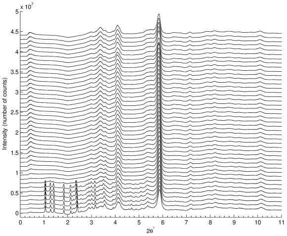
Figure 5.1: Sums of back-projected diffraction patterns of the 43 data sets of nickel nitrate calcination presented in a stack plot.

The stack plot of the back-projected data for the nickel nitrate calcination experiment is shown in Figure 5.1, while the PDP diagram is given in Figure 5.2. Because of its size, the last figure is split into two segments on two pages (pages 5.1 and 5.2). A number of phase distribution patterns are observed in these data; the main ones can be seen in Figure 5.2. A prominent feature of this figure is the rotation of the sample during the early part of the calcination process as indicated by the hole position near the cylinder perimeter. This is obviously due to an unstable mechanical setting which allowed the sample to spin during the scan. In the following we discuss the main PDPs and try to link them to actual phases:

1. The first PDP (first column from left) belongs to alumina (Al₂O₃). The following peaks of $\gamma$-alumina [106] were identified with this PDP: ($2\theta^{\circ}$, $hkl$, $d$ Å) = (2.92, 112, 2.8042), (3.40, 211, 2.4066), (3.56, 202, 2.2955), (4.09, 220, 1.9983), (4.16, 004, 1.9677), (5.32, 321, 1.5374), (5.79, 400, 1.4130), (5.83, 224, 1.4021), (6.47, 420, 1.2638), (6.73, 413, 1.2150), (7.13, 404, 1.1477), (7.92, 415, 1.0338), (8.19, 440, 0.9991), (8.76, 336, 0.9347), (8.87, 611, 0.9228), (9.19, 444, 0.8909), (10.06, 624, 0.8137) and (10.14, 408, 0.8074). It should be remarked that the fading intensity seen in frames (rows) 37 and 38 is most likely to be from a sudden and temporary drop in the beam intensity or from an error in the detector, and hence should not be ascribed to a dynamic transformation in the sample. This view is supported by the fact that this sudden drop in intensity is observed with the other PDPs of the other phases.

2. The second PDP displays a spatial distribution similar to that of $\gamma$-alumina but with an obvious increase in intensity. A peak at about $2\theta^{\circ}$ = 0.42 with this PDP was observed but could not be identified as arising from $\gamma$-alumina. This peak is highly asymmetric and apparently consists of two overlapping peaks. Most probably, this peak originates from another form of alumina. The observed intensity decrease of $\gamma$-alumina’s most prominent peak, at about $2\theta^{\circ}$ = 5.83, with the observed increase in this unknown peak may suggest that $\gamma$-alumina is transforming to another form of alumina. It is noteworthy that the gradual drop in the beam intensity was tested against the gradual decrease in the storage ring current, by comparing the total intensity of the first and last data sets of all data collections (i.e. molybdenum, nickel nitrate calcination, nickel nitrate reduction, and nickel chloride). Although this drop was confirmed in all cases, it cannot alone explain the tangible drop in the $\gamma$-alumina intensity, since such a big drop in intensity is not observed with the other phases. It should be remarked that a large number of standard patterns of alumina were inspected, with various space groups, as found on the ICSD database, but no structure could be found with a peak at such a low scattering angle. However, one exception is that of Repelin and Husson [117] which has two peaks at $2\theta^{\circ}$ = 0.35 and 0.69. This may be a possibility for the phase that is responsible for this peak which seems to comprise two overlapping peaks.

3. The third PDP is observed at $2\theta^{\circ}$ = 1.05, 1.25, 1.41, 1.82, 1.96, 2.12, 2.24, 2.38, 2.55, 2.82, 2.85, 2.88, 3.00, 3.15, 3.52, 3.88, 3.93, 4.37, 4.53, 4.65, 4.84 and 5.07. All these peaks are identified as originating from the nickel ethylenediamine dinitrate, [Ni(en)₃](NO₃)₂, precursor according to the diffraction pattern of this compound which was obtained from Krishnan et al [85], after re-scaling the scattering angles to match the wavelength; no data about $hkl$’s and $d$-spacings are available for this pattern. This PDP was also observed at higher scattering angles but these angles are beyond the range of the diffraction pattern of Krishnan et al. This PDP suggests that the precursor is consumed at the beginning of the calcination process. It should be remarked that there is an obvious shift of the precursor peak positions towards lower scattering angles as the temperature increases. This is consistent with an increase in the $d$-spacings as the temperature rises. The position shift feature is also observed in other phases such as alumina. Another remark is that the relative intensity of the diffraction peaks suggests that the precursor is damaged by radiation as demonstrated by Figure 4-b of Krishnan et al.

4. The fourth PDP is observed at about $2\theta^{\circ}$ = 5.52 and 6.47. Apparently, this phase is bunsenite, NiO-[FM3-M], [139] as there are two strong peaks of this compound at these positions with ($hkl$, $d$ Å) = (220, 1.4829) and (311, 1.2647) respectively. Interestingly, some alumina peaks which are close to expected peaks of NiO appear as if they are contaminated with this phase. An example of this is shown in the last column of Figure 5.2 where the $\gamma$-alumina peak at $2\theta^{\circ}$ = 8.76 seems to be contaminated with the NiO peak at $2\theta^{\circ}$ = 8.73 ($hkl$ = 420, $d$ Å = 0.9379) which is a strong peak. Also, the alumina peak at $2\theta^{\circ}$ = 3.40 shows strong sign of contamination with the strong peak of NiO at $2\theta^{\circ}$ = 3.38 ($hkl$ = 111, $d$ Å = 2.4216). Also the next PDP contains a peak from NiO. Apparently, the formation of bunsenite is due to thermal decomposition of the precursor at high temperature. The missing link between the two phases (i.e. frames 9-16 where no transitional phase is observed at this spatial distribution) suggests that an amorphous form of the precursor or a transitional compound has participated in this process. The more apparent egg-shell distribution of the NiO may suggest an oxidation process where a molecular oxygen from air is involved in this reaction.

5. The fifth PDP is observed at about $2\theta^{\circ}$ = 3.90. This PDP results from a combination of the last two PDPs due to overlapping peaks from the two phases. It therefore consists of the ($2\theta^{\circ}$, $hkl$, $d$ Å) = (3.90, 200, 2.0972) which is the strongest peak of NiO, and the precursor peak at $2\theta^{\circ}$ = 3.88 or 3.93.

6. The sixth PDP is observed at about $2\theta^{\circ}$ = 2.86, 4.49 and 4.62. It could not be identified, although it may be a transitional form of the precursor.

It is noteworthy that no pure nickel metal can be traced, in either of the two forms for which there exists data, i.e. Ni-[FM3-M] and Ni[P63/MMC]; similarly other potential nickel compounds were considered but not found.

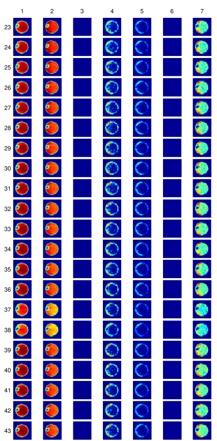
Figure 5.2: Phase distribution patterns of the nickel nitrate calcination data. The rows and columns are labelled with their indices and the background is masked.

5.2 Nickel Nitrate Reduction

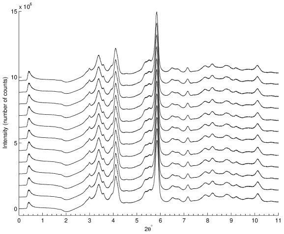
Figure 5.3: Sums of back-projected diffraction patterns for the 12 data sets of nickel nitrate reduction, presented as a stack plot.

The stack plot of back-projected data for the nickel nitrate reduction experiment is shown in Figure 5.3. A number of phase distribution patterns are observed in this collection; the main ones are displayed in Figure 5.4. The prominent feature is that in most cases hardly any changes occur during the reduction process. This includes the positions of the peaks which are almost constant since the sample is held at constant steady state temperature. In the following we discuss these PDPs and try to link them to crystallographic phases:

1. The first PDP (first column from left) originates from alumina. The following peaks of $\gamma$-alumina [106] were identified with this PDP: ($2\theta^{\circ}$, $hkl$, $d$ Å) = (1.78, 101, 4.5910), (2.89, 200, 2.8260), (2.92, 112, 2.8042), (3.40, 211, 2.4066), (3.44, 103, 2.3798), (3.56, 202, 2.2955), (4.09, 220, 1.9983), (4.16, 004, 1.9677), (4.49, 213, 1.8203), (5.03, 312, 1.6274), (5.32, 321, 1.5374), (5.79, 400, 1.4130), (5.83, 224, 1.4021), (6.47, 420, 1.2638), (6.73, 413, 1.2150), (7.13, 404, 1.1477), (7.42, 107, 1.1028), (7.92, 415, 1.0338), (8.19, 440, 0.9991), (8.76, 336, 0.9347), (8.87, 611, 0.9228), (9.19, 444, 0.8909), (9.64, 604, 0.8497), (10.06, 624, 0.8137), (10.14, 408, 0.8074) and (10.72, 329, 0.7637).

2. The second PDP, which is observed at about $2\theta^{\circ}$ = 0.42, is similar to the second PDP of the calcination data, and apparently consists of two peaks. As its intensity is increasing while some of alumina peaks appear to be decreasing, as seen in the first PDP, it is likely to be another form of alumina transforming from $\gamma$-alumina.

3. This egg-shell phase distribution pattern is observed at $2\theta^{\circ}$ = 3.90, 5.52 and 6.47. Similar to the calcination data, it seems to be originating from bunsenite NiO-[FM3-M] [139] with the following values ($hkl$, $d$ Å) = (200, 2.0972), (220, 1.4829) and (311, 1.2647) respectively. Also some alumina peaks seem to be contaminated with peaks expected from NiO at those positions. An example is presented in the last column where the $\gamma$-alumina peak at $2\theta^{\circ}$ = 3.40 seems to be contaminated with the second strongest peak of NiO at $2\theta^{\circ}$ = 3.38 ($hkl$ = 111, $d$ Å = 2.4216). There is also a strong sign of contamination of alumina peaks at $2\theta^{\circ}$ = 6.73 and 8.76 with the NiO peaks at $2\theta^{\circ}$ = 6.76 and 8.73, respectively. The last peaks have ($hkl$, $d$ Å) = (222, 1.2108) and (420, 0.9379) respectively.

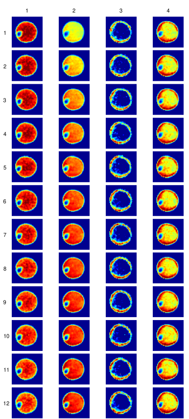
Figure 5.4: Phase distribution patterns of nickel nitrate reduction data. The rows and columns are labelled with their indices and the background is masked.

5.3 Nickel Chloride

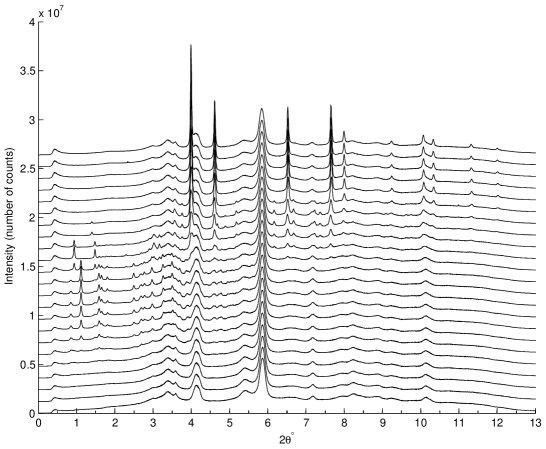
Figure 5.5: Sums of back-projected diffraction patterns of the 23 data sets of nickel chloride presented in a stack plot.

The stack plot of the back-projected data for the nickel chloride experiment is shown in Figure 5.5. A number of very interesting phase distribution patterns are observed in the data with the main candidates displayed in Figure 5.7. In the following we discuss the main PDPs and attempt to link them to actual phases, where the identifications are made jointly by Simon Jacques and the author of this thesis:

1. The first PDP (first column from left) belongs to alumina. The following peaks of $\gamma$-alumina [106] were identified with this PDP: ($2\theta^{\circ}$, $hkl$, $d$ Å) = (1.78, 101, 4.5910), (2.92, 112, 2.8042), (3.40, 211, 2.4066), (3.56, 202, 2.2955), (4.09, 220, 1.9983), (5.39, 105, 1.5165), (5.83, 224, 1.4021), (7.13, 404, 1.1477), (7.92, 415, 1.0338), (8.19, 440, 0.9991), (8.87, 611, 0.9228), (9.19, 444, 0.8909) and (10.14, 408, 0.8074). Other alumina peaks overlap with peaks from other phases and hence are masked. Some of these masked peaks have a shadowy trace on the image of the masking peaks.

2. The second PDP is observed at about $2\theta^{\circ}$ = 0.42. As already stated, this seems to be another form of alumina transforming from $\gamma$-alumina since the increase in its intensity is associated with a decrease of the $\gamma$-alumina intensity (see Figure 5.7). This possibility is supported by the fact that the spatial distribution of this phase is identical to that of $\gamma$-alumina.

3. The third PDP is originating from the nickel chloride ethylenediamine tetrahydrate, NiCl₂(en)(H₂O)₄, precursor. Interestingly, the polycrystalline form of precursor is absent in the first few frames as it forms during the heat treatment. This PDP is observed at about $2\theta^{\circ}$ = 0.85, 1.58, 1.80, 2.49, 2.67, 2.77 and 4.75.

4. The fourth PDP is observed at about $2\theta^{\circ}$ = 1.11, 1.58, 3.25, 3.49, 3.69 and 3.89. It seems to be related to the previous phase. There is also a sign of contamination with this phase at about $2\theta^{\circ}$ = 3.58, but it is difficult to verify as the position is surrounded by other peaks.

5. The fifth PDP is Ni₂Cl₂(en). This PDP is observed at about $2\theta^{\circ}$ = 0.93, 1.48, 2.29, 2.89, 3.02 and 3.16. The shadow seen at frames 4-7 is an artifact resulting from a neighbouring peak which is not related to this phase.

6. The sixth PDP is NiCl₂. The following three peaks of NiCl₂-[R3-MH] [52] are identified with this PDP: ($2\theta^{\circ}$, $hkl$, $d$ Å) = (1.41, 003, 5.8000), (4.70, 110, 1.7415) and (4.90, 113, 1.6679). Other peaks are either too faint to observe or they are masked by the presence of larger peaks from other phases in their position.

7. The seventh PDP is hexagonal close packed (HCP) nickel. The following peaks of Ni-[P63/MMC] [71] are identified with this PDP: ($2\theta^{\circ}$, $hkl$, $d$ Å) = (3.79, 002, 2.1605), (5.23, 102, 1.5652), (6.24, 110, 1.3110), (6.73, 103, 1.2163), (7.21, 200, 1.1354), (7.45, 201, 1.0981), (9.54, 210, 0.8583) and (9.73, 211, 0.8418). The strongest peak of Ni-[P63/MMC] at $2\theta^{\circ}$ = 4.07 is masked by the strong $\gamma$-alumina peak at $2\theta^{\circ}$ = 4.09.

8. The eighth PDP is face centred cubic (FCC) nickel. The following peaks of Ni-[FM3-M] [147] are identified with this PDP: ($2\theta^{\circ}$, $hkl$, $d$ Å) = (3.99, 111, 2.0521), (4.60, 200, 1.7771), (6.51, 220, 1.2566), (7.64, 311, 1.0717), (7.98, 222, 1.0260), (9.21, 400, 0.8886), (10.04, 331, 0.8154), (10.30, 420, 0.7948), (11.29, 422, 0.7255) and (11.98, 511, 0.6840). In Figure 5.6 the full width at half maximum (FWHM) of the ($2\theta^{\circ}$, $hkl$, $d$ Å) = (6.51, 220, 1.2566) peak of this phase is tomographically mapped for the last ten frames (14-23) where the phase is formed. According to the Scherrer equation the mean size of crystallites, $\tau$, is given by

   $$\tau=\frac{\kappa\lambda}{\beta\cos\theta}$$ (5.1)

   where $\kappa$ is a shape factor which ranges between about $0.87-1.0$ depending on the shape of crystallites, $\lambda$ is the wavelength of the radiation, $\beta$ is the peak broadening at half maximum due to the size of crystallites, and $\theta$ is the diffraction angle. As the actual broadening involves instrumental as well as size factors, the total full width at half maximum, $F_{t}$, is given by

   $$F_{t}^{2}=F_{i}^{2}+\beta^{2}$$ (5.2)

   where $F_{i}$ is the instrumental broadening. In the nickel chloride experiment, $\lambda=0.14272$ Å, $F_{i}\simeq 0.021^{\circ}\simeq 0.00037$ radian, $\theta\simeq 3.26^{\circ}$ for the (220) peak of FCC nickel, and $F_{t}$ ranges between about $0.025^{\circ}-0.209^{\circ}$ ($0.00044-0.00365$ radian). Inserting these values in Scherrer equation with $\kappa=0.90$, which is a typical value, we obtain a crystallite size range of about $3.5-54$ nanometre. Figure 5.6 reveals that the FCC nickel starts forming at the perimeter of the cylinder with a subsequent invasion to the inside region. The figure also reveals that the size of the crystallites at the interior regions eventually grows to become larger than those near the surface of the extrudate cylinder. It should be remarked that the larger crystallite size found in the interior is due to the prior presence of NiCl₂ which promoted crystal growth. Another remark is that the disappearance of HCP-nickel with the growth of FCC-nickel (as can be observed by comparing PDP 7 to PDP 8) suggests that HCP-nickel is transforming to FCC-nickel which is the more stable form.

9. The ninth PDP, which is observed at about $2\theta^{\circ}$ = 4.39, is suspected to belong to another phase which could not be identified. A trace of this PDP was also observed at about $2\theta^{\circ}$ = 2.96, 4.94 and 5.06. These positions are surrounded by other peaks from other phases and hence cannot be unambiguously identified.

It is noteworthy that some images show clear sign of sample rotation at frame 18.

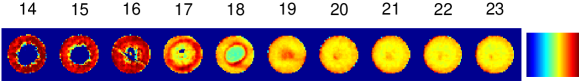
Figure 5.6: Crystallite size distribution of FCC nickel by mapping the FWHM of the (220) reflection at $2\theta=6.51^{\circ}$. The colour bar ranges between 0^∘ (blue) and 0.065^∘ (red). The blue maps the regions where no FCC nickel peaks exist and hence the FCC phase is absent, while the red represents the regions of smallest crystal size and the yellow represents the regions of largest crystal size. The numbers shown on the top are the indices of the data sets.

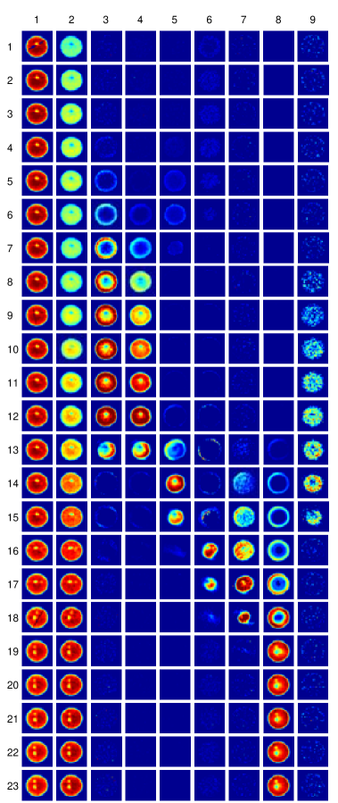
Figure 5.7: Phase distribution patterns of nickel chloride data. The rows and columns are labelled with their indices and the background is masked.

Chapter 6 Some Problems and Solutions associated with Diffraction-Based Imaging

In this chapter a number of problems related to the use of diffraction in X-ray imaging are discussed and some solutions are offered. The main focus will be on two data sets collected by Olivier Lazzari and Simon Jacques using CAT-type TEDDI and TADDI techniques. Also, a third data set collected by Conny Hanson, Matt Wilson and Simon Jacques [private communication], using a simple radiographic technique, will be briefly discussed.

6.1 Large Object Problem and Multi TEDDI Solution

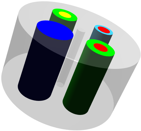
Figure 6.1: A 3D image of the test object. The colours refer: blue to aluminium, green to PEEK, red to bone ash, yellow to iron oxide and sky blue to glass.

A key problem associated with the type of imaging employed in this thesis is that significant peak broadening and splitting are observed when studying objects above a certain size. These effects arise due to the different paths that X-rays take from sample to detector. Figure 6.15 illustrates how peak broadening and splitting can arise in a recorded diffraction pattern. In this section we present two data sets collected by two different diffraction modes: angle dispersive (ADD) and energy dispersive (EDD) where the sample used is a large object. Both experiments use the same sample which is a specially designed test object consisting of known materials. The purpose of these experiments is to investigate sample size effects and assess the data acquisition and data analysis methods since the ingredients and morphology of the object are well known. The test object, depicted schematically in Figure 6.1, consists of a cylinder of wax ($r=18$ mm) with a hollow axis ($r=1.25$ mm). The cylinder accommodates in each one of its quartets another cylinder with its axis parallel to the cylindrical wax axis: an aluminium cylinder ($r=5$ mm), an iron oxide cylinder ($r=2$ mm) inside a polyether ether ketone (PEEK) polymer container of external radius $r=4$ mm, a bone ash cylinder ($r=2$ mm) inside a glass container of external radius $r=3$ mm, and another bone ash cylinder ($r=2$ mm) inside a PEEK container of external radius $r=4$ mm. The details of this test object can be found in Lazzari et al [88]. The purpose of using such a heterogeneous multi-phase object is to have regions of different X-ray absorption and varying degrees of crystallinity. This imposes a more rigorous test of the data acquisition and reconstruction methods, as well as being a more faithful simulation of real life objects.

6.1.1 ADD Data

The ADD data were collected at station ID15A of ESRF which uses a monochromatic beam in the energy range $30-500$ keV for angle dispersive investigations. The station can also use a white beam in that energy range for EDD studies [50]. The wavelength of the monochromatic beam used in this experiment is $\lambda=0.17712$ Å. A circular slice of the object (perpendicular to the cylindrical axis) was chosen for a CAT-type scan as presented in § 4.2.3 and demonstrated in Figure 4.3. The measurements consist of 81 rotations around the object axis between 0-180^∘ in regular intervals times 80 translations in steps of 0.5 mm. The total collected data set therefore consists of 6480 ($81\times 80$) patterns. The collection time of each pattern was about 0.5 second, giving a total collection time for the whole data set of about one hour. This raw data set, which is a sinogram of rotation versus translation, was back-projected (excluding the last rotational step) using the EasyDD program. An image of this sinogram, as represented by the total intensity of the individual patterns, is given in Figure 6.2. The resultant data, which consist of 6400 ($80\times 80$) patterns, represent a tomographic image of the slice in real space. An image of the back-projected data represented by the total intensity of the individual patterns is shown in Figure 6.3. A sum of all back-projected diffraction patterns can also be seen in Figure 6.4. More details about this experiment can be found in Lazzari et al [89]. Using EasyDD in multi-batch mode, the back-projected peaks of the six phases are curve-fitted using a Gaussian profile with a linear background. The main results are presented as tomographic images in Figures 6.5-6.10. In the following points we discuss some issues related to these results:

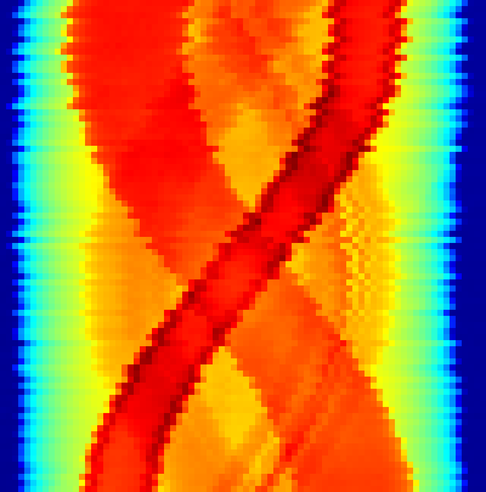
Figure 6.2: A sinogram consisting of 81 rotation rows $\times$ 80 translation columns for the ADD data. The displayed parameter is the total intensity of the individual patterns.

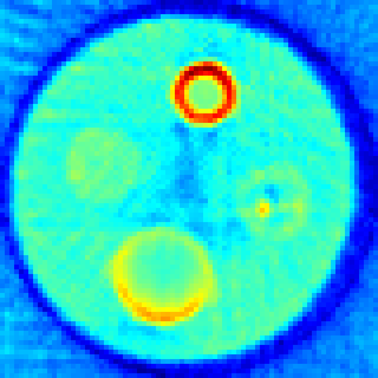
Figure 6.3: A tomographic image ($80\times 80$) obtained using the total intensity of the back-projected ADD data.

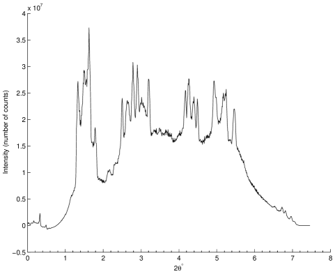
Figure 6.4: Sum of all diffraction patterns of the back-projected ADD data.

• Wax: (Figure 6.5) No standard diffraction pattern was available to compare with the experimental data and identify the Bragg’s reflections. Therefore, the identification of this phase is based on the spatial distribution in the tomographic images. It should be remarked that the distortion in the second frame of Figure 6.5 is due to peak overlap and restrictions in curve-fitting.

• Aluminium: (Figure 6.6) Peaks at the following approximate scattering angles $2\theta^{\circ}$ = 2.50, 2.65, 2.78, 2.90, 2.99, 3.10, 3.20, 4.17, 4.26, 4.38, 4.48, 4.93, 5.21, 5.46, 6.73 and 6.96 are identified with this phase according to the spatial distribution in the tomographic images. Considering the uncertainties in the standard diffraction patterns and experimental data the peak at $2\theta^{\circ}$ = 4.38 can be identified with the following peak of aluminium [FM3-M] [142]: ($2\theta^{\circ}$, $hkl$, $d$ Å) = (4.33 , 111, 2.3417) which is the strongest peak.

• PEEK: (Figure 6.7) No standard diffraction pattern was available to compare with the experimental data and identify the Bragg reflections. Therefore, the identification of this phase is based on the spatial distribution in the tomographic images.

• Bone ash: (Figure 6.8) Peaks at the following approximate scattering angles, $2\theta^{\circ}$ = 1.08, 1.95, 2.18, 2.50, 3.33 and 3.56, are identified with this phase according to the spatial distribution in the tomographic images. Considering the uncertainties in the standard diffraction patterns and experimental data the peaks at $2\theta^{\circ}$ = 1.95, 2.50, 3.33 and 3.56 can be identified with the following peaks of calcium phosphate Ca₃(PO₄)₂-[R3CH] (which is the main component of bone ash) respectively [145]: ($2\theta^{\circ}$, $hkl$, $d$ Å) = (1.95, 110, 5.2176), (2.49, 024, 4.0685), (3.37, 300, 3.0124) and (3.53, 217, 2.8779).

• Iron oxide (hematite Fe₂O₃): (Figure 6.9) Peaks at the following approximate scattering angles $2\theta^{\circ}$ = 2.12, 2.28, 2.42, 2.59, 3.48, 3.75, 3.99, 4.09, 4.32, 5.75, 6.00 and 6.34 are identified with this phase according to the spatial distribution in the tomographic images. Considering the uncertainties in the standard diffraction patterns and experimental data the peaks at $2\theta^{\circ}$ = 3.75, 3.99, 6.00 and 6.34 can be identified with the following peaks of hematite [R3-CH] [111] respectively: ($2\theta^{\circ}$, $hkl$, $d$ Å) = (3.76, 104, 2.6998), (4.03, 110, 2.5173), (5.99, 116, 1.6948) and (6.34, 122, 1.6026).

• Glass: An amorphous scattering signal was observed at several $2\theta$ positions with no obvious peak. Examples of this signal (which associates with signals from other phases) are given in Figure 6.10.

Because a large test object was used in this experiment, peak broadening and splitting were observed in the raw data and hence in the reconstructed data. As the EDD technique employs a fixed and usually small scattering angle which could reduce the effect of sample size on the signal spread (refer to Figure 6.15), it was decided to perform a similar experiment using EDD to investigate and assess the potential improvement of data quality offered by this technique. The EDD experiment, with a fairly detailed analysis, is presented in the next section, while a comparison between ADD and EDD experiments is given in section 6.1.3.

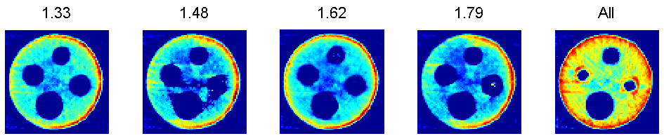
Figure 6.5: Tomographic images from ADD data of the wax cylinder as represented by the Gaussian area of the peaks. The numbers on the top of the first 4 images are the approximate positions of the peaks in terms of $2\theta^{\circ}$, while the last image represents the total of the first 4 peaks as modelled by a single Gaussian peak.

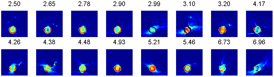
Figure 6.6: Tomographic images from ADD data of the aluminium cylinder as represented by the Gaussian area of the peaks. The numbers on the top of each image are the approximate positions of the peaks in terms of $2\theta^{\circ}$.

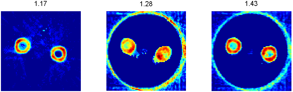
Figure 6.7: Tomographic images from ADD data of the PEEK cylinders as represented by the Gaussian area of the peaks. The numbers on the top of the images are the approximate positions of the peaks in terms of $2\theta^{\circ}$. In frames 2 and 3, traces of other components are masked for clarity.

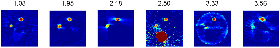
Figure 6.8: Tomographic images from ADD data of the bone ash cylinders as represented by the Gaussian area of the peaks. The numbers on the top of the images are the approximate positions of the peaks in terms of $2\theta^{\circ}$. The fourth frame includes an aluminium trace.

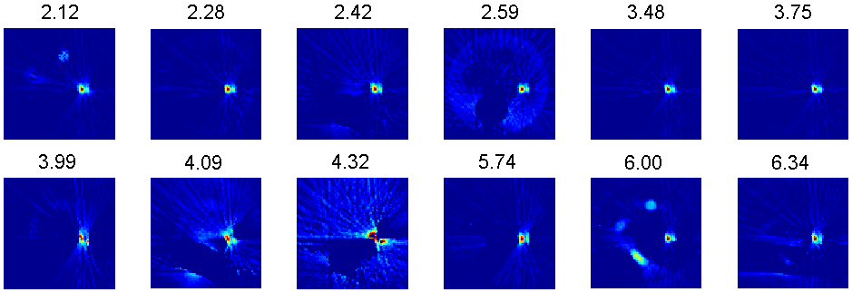
Figure 6.9: Tomographic images from ADD data of the iron oxide cylinder as represented by the Gaussian area of the peaks. The numbers on the top of the images are the approximate positions of the peaks in terms of $2\theta^{\circ}$.

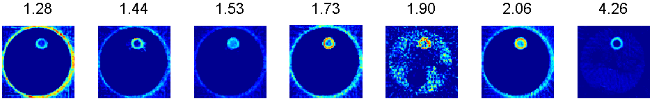
Figure 6.10: Tomographic images from ADD data of the glass cylinder as represented by the Gaussian area of the peaks. The numbers on the top of the images are the approximate positions of the peaks in terms of $2\theta^{\circ}$. Traces of other components are masked in most frames.

6.1.2 EDD Data

The EDD data were collected at station 16.4 of Daresbury SRS before its closure in 2008. This station used a white beam for energy dispersive powder diffraction and was designed for the study of chemical reactions and phase transitions of materials held at high temperatures and pressures [138]. In this experiment a white beam of diameter 0.5 mm in the energy range 1-110 keV was used. The collection angle of the fixed EDD detector was $2\theta$ = 4.5^∘. The reason for choosing this small angle is to collect the diffraction patterns at higher energies to reduce the absorption of diffracted signals along its path inside the sample. This will also mitigate the effect of signal spread. A drawback of this shift to high energies is a distortion of the sampling volume shape (lozenge) which requires correction at the data processing stage.

A circular slice of the object (perpendicular to the cylindrical axis) was chosen for a CAT-type scan as presented in § 4.2.3 and demonstrated in Figure 4.3. The measurements consist of 79 rotations around the object axis between 0-180^∘ in regular intervals times 80 translations in steps of 0.5 mm. The total size of the collected data therefore consists of 6320 ($79\times 80$) patterns. The collection time of each pattern was about 10 seconds, totaling a collection time for the whole data set to about 18 hours. This raw data set, which is a sinogram of rotation versus translation, was back-projected using the EasyDD program. An image of this sinogram, as represented by the total intensity of the individual patterns, is presented in Figure 6.11. The resultant data, which consist of 6400 ($80\times 80$) patterns, represent a tomographic image of the slice in real space. An image of the back-projected data, as represented by the total intensity of the individual patterns, is given in Figure 6.12. A sum of the back-projected diffraction patterns can also be seen in Figure 6.13. It is noteworthy that the orientation of the test object in the EDD experiment is different to that in the ADD case, and therefore the position of the elements in the related images are different. More details about this experiment can be found in Lazzari et al [88, 89]. Using EasyDD in multi-batch mode, the back-projected peaks of the six phases are modelled by a Gaussian profile with a linear background. The main results are presented as tomographic images in Figure 6.14. In the following points we discuss some issues related to these results:

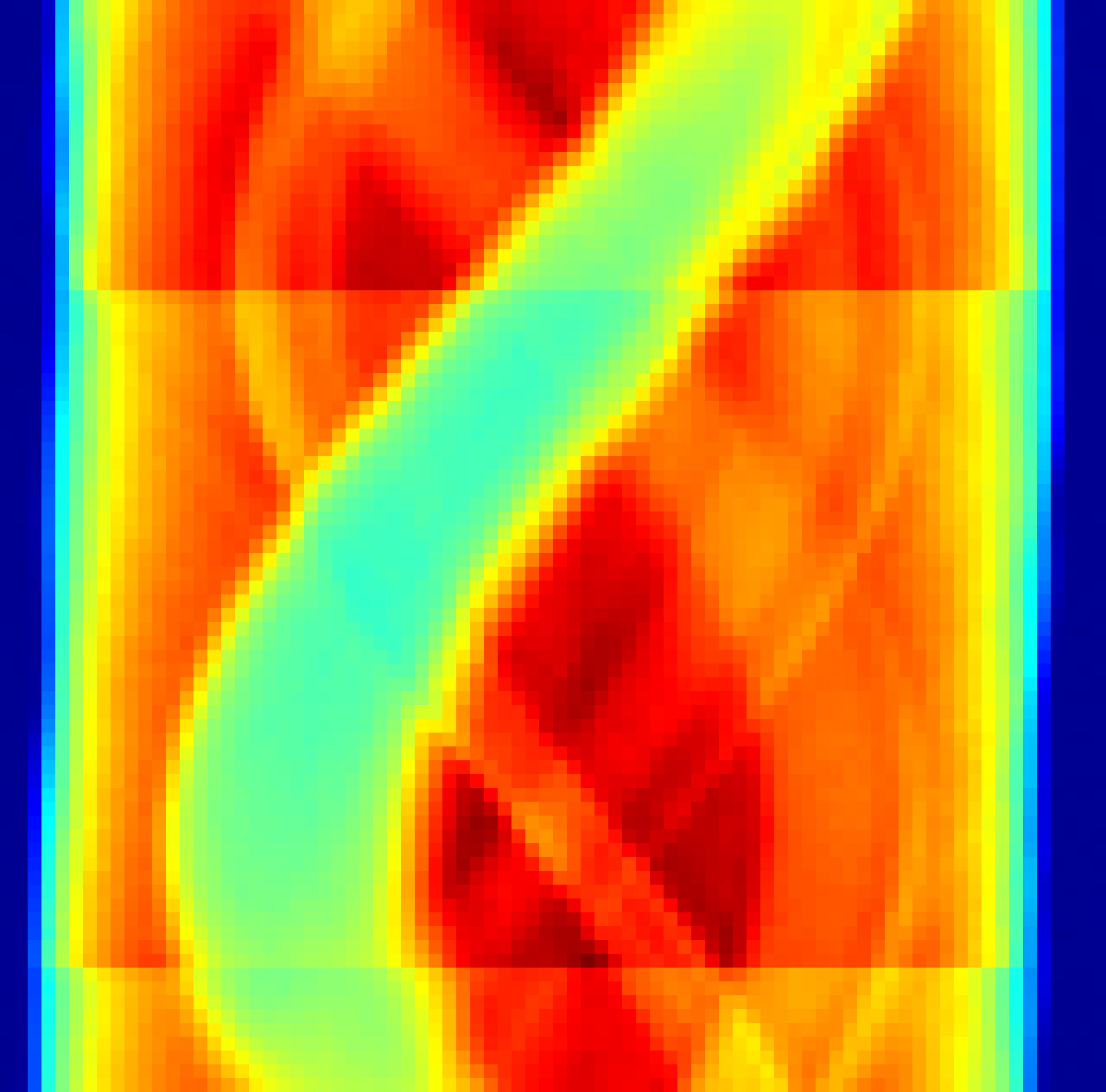
Figure 6.11: A sinogram consisting of 79 rotation rows $\times$ 80 translation columns for the EDD data. The displayed parameter is the total intensity of the individual patterns. The observed shift is due to mechanical instability of the translation-rotation stage.

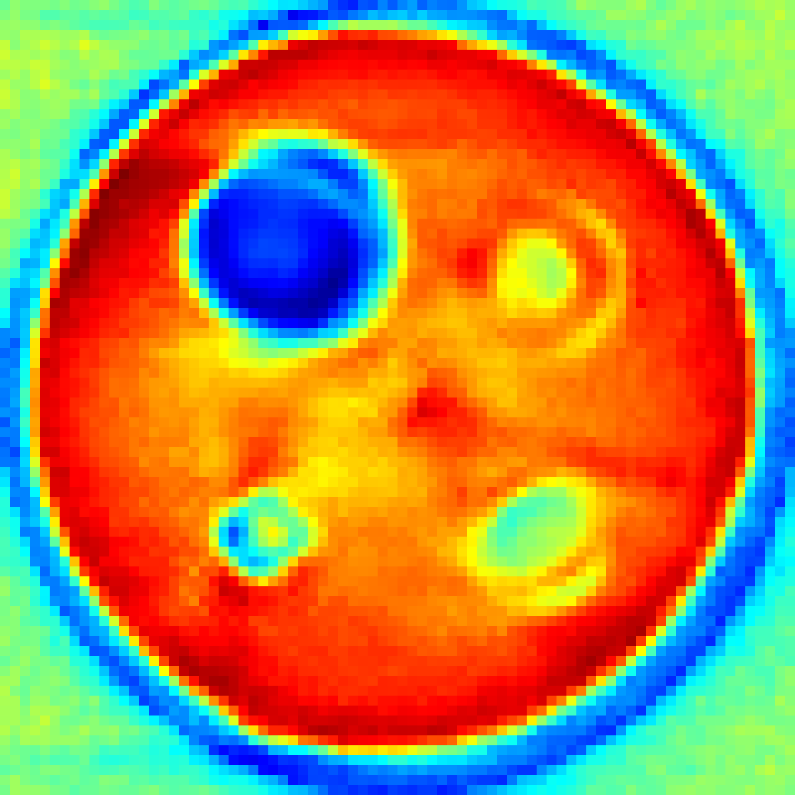
Figure 6.12: A tomographic image ($80\times 80$) of the total intensity of the back-projected EDD data.

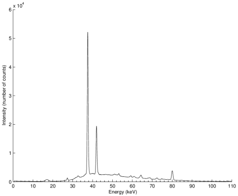
Figure 6.13: Sum of the diffraction patterns of the back-projected EDD data.

• Wax: No standard diffraction pattern was available to compare with the experimental data and identify the Bragg reflections. Therefore, the identification of this phase is based on the spatial distribution in the tomographic images.

• Aluminium: Peaks 1, 2, and 3 of this phase are approximately in the same position as peaks 2, 3 and 4 of wax. In fact the aluminium peaks at these three positions have negative amplitude as though they were absorption peaks. This negative-peak feature was observed for other peaks with other phases. The following peaks of aluminium [FM3-M] are identified [142]: ($E$ keV, $hkl$, $d$ Å) = (37.5, 200, 2.0280), (68.9, 111, 2.3417), (74.8, 200, 2.0280) and (80.0, 200, 2.0280). Reflections of aluminium at about $E=$ 27.3 and 42.0 keV were also detected but no data could be retrieved from ICSD.

• PEEK: No standard diffraction pattern was available to compare with the experimental data and identify the Bragg reflections. Therefore, the identification of this phase is based on the spatial distribution in the tomographic images.

• Bone ash: The following peaks of calcium phosphate Ca₃(PO₄)₂-[R3CH] (which is the main component of bone ash) are identified [145]: ($E$ keV, $hkl$, $d$ Å) = (46.5, 211, 3.4016), (48.2, 119, 3.2507), (51.0, 125, 3.1071), (52.3, 300, 3.0124) and (60.9, 220, 2.6088).

• Iron oxide (hematite Fe₂O₃): The following peaks of hematite [R3-CH] are identified [111]: ($E$ keV, $hkl$, $d$ Å) = (59.2, 104, 2.6996), (63.7, 110, 2.5175), (73.0, 113, 2.2066), (88.2, 024, 1.8412) and (96.1, 211, 1.6364).

• Glass: An amorphous scattering signal was observed over several energy positions with no obvious dominant peak. Examples of this signal (which associates signals from other phases) are given in the last row of Figure 6.14.

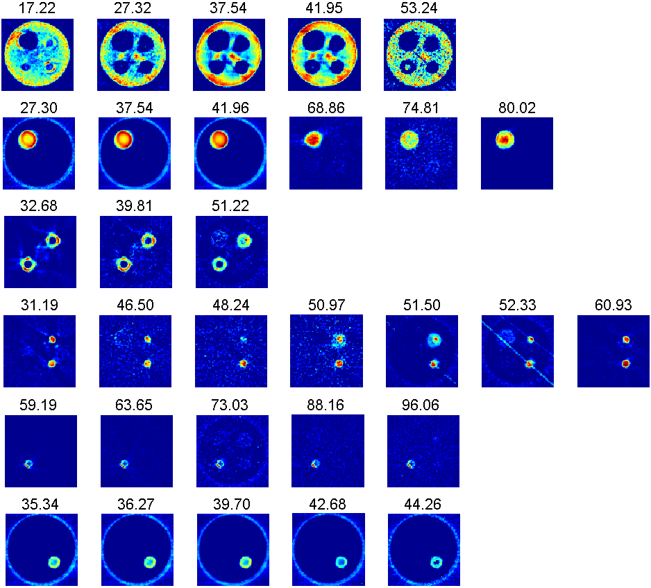
Figure 6.14: Tomographic images of the six components of the test object from the EDD data as represented by the Gaussian peak area. The rows in top-down order stand for: wax, aluminium, PEEK, bone ash, iron oxide and glass. The numbers on the top of each frame are the energy position of the peak in keV. In some frames, traces of other components are masked for clarity.

6.1.3 Comparison and General Conclusions

In this section, we compare the ADD and EDD imaging data and try to reach general conclusions about these techniques.

• Negative peaks were observed in both ADD and EDD data. Its most prominent occurrence is with aluminium and wax where strong negative peaks of aluminium appear in the same positions as the normal peaks of wax and vice versa (e.g. at $2\theta^{\circ}$ $\simeq$ 1.33 and 3.22 in ADD data, and at $E$(keV) $\simeq$ 37.5 for EDD data). This feature was also observed between wax and components other than aluminium. Some of the results and images presented in this section were obtained by fitting these negative peaks like normal peaks then taking the absolute value of the Gaussian area.

• Peak broadening and splitting were observed in both ADD and EDD data but they were more prominent in the ADD data. These effects, which are manifested in the raw diffraction data and hence in the reconstructed data, can be explained by the large sample size and large scattering angle, as illustrated graphically in Figure 6.15. Although the size of the sample is the same for the ADD and EDD data, the (fixed) scattering angle of the EDD data is small (=4.5^∘) and hence the spread of the detected signal is less, resulting in reduced peak broadening and splitting. However, the use of a small scattering angle can result in another problem that is peak overlap. It should be remarked that these problems can be corrected for by employing correction algorithms at the data processing and analysis stage. However, this is not a trivial task and hence it is left for future research as it is beyond the remit of this thesis.

• To avoid peak splitting effects and the occurrence of repetitive peaks, we have adopted a minimum gap between neighbouring peaks for them to be considered as two different peaks.

• The general impression is that the ADD data are more complicated and have more peaks than the EDD data. This is due partly to the broadening and splitting effects which are more severe in the ADD data, as already indicated. It may also be attributed in part to the fact that the diffracting lozenge size and shape in an EDD scan is constant whereas the sampling volume is variable in an ADD scan.

• The quality of the ADD and EDD data varies from one component to another although EDD results are generally clearer and simpler. Due to the variation in radiation sources, detectors and other equipment, it is difficult to make a generalised comparison of the two techniques based on the results of just these experiments.

• A prominent feature of ADD data is the appearance of streaks in many images (e.g. Figure 6.6 $2\theta^{\circ}$ = 6.96 and Figure 6.9 $2\theta^{\circ}$ = 5.74). These streaks change orientation depending on the channels chosen to represent the peak. This feature may be explained by the fact that the sampling volume, and the nature and length of the path of reflected signal in the ADD technique, are variable. Streaks may also be attributed to peak distortion due to peak overlap, peak splitting, background noise and curve-fitting strategy (peak range, position and restrictions).

• An important problem in diffraction-based imaging, which requires correction at processing and analysis stage, is the absorption of reflected signals inside the sample. This problem is particularly serious when the sample is large due to the long signal paths. This reduces signal-to-noise ratio and degrades the quality of the diffraction patterns. Also, the difference in the length and nature of the signal paths, which may be more severe in the ADD technique due to unparallel paths, results in uneven absorption and hence further distortion in the patterns. Uneven absorption is more grave when the sample is large with complex structure and morphology. In such cases, correction for absorption may become impossible to introduce. Because absorption is energy-dependent, the EDD technique may suffer from selective absorption which can be another source of pattern distortion. Some solutions to the problems associated with absorption have been given by Lazzari et al [88, 89].

Figure 6.15: A schematic diagram illustrating the effect of sample size and scattering angle on the signal spread which is manifested in peak broadening and splitting. The large signal spread observed in (a), due to the large sample size and large scattering angle, is diminished in (b) by reducing the size of the sample and in (c) by reducing the scattering angle.

6.2 Prospects for Diffraction-Based Imaging

The examples given in this thesis, and the related cited work, are clear demonstration of the capability and potential of diffraction-based imaging; both in angle dispersive and energy dispersive modes. As data acquisition and detector technologies are rapidly improving with the wide availability of bright light sources, the future of these imaging techniques is very promising. The rapid improvement in computational technology and easy access to massive computational resources is another factor that can contribute to the development and widespread use of diffraction-based imaging. In particular, EDD imaging can also exploit other signals, such as fluorescence and scattering bands, and hence enjoys yet further potential. Multi-pixel detector technology, such as HEXITEC multi-TEDDI detectors, will be a contributing factor to realising a huge increase in the speed of data acquisition, and thereby an improved spatial and temporal resolution since this technology will enable the acquisition of images with a finer pixel size and in shorter time intervals. An obvious beneficiary of these technologies will be dynamic and time-dependent studies and tomographic imaging. The main difficulties to overcome include data processing and analysis capabilities to match the massive accumulation of data associated with these new imaging techniques. An investment in software development will be a top priority for future progress. The resultant data processing should consider pixel size and shape corrections which are required to account for the finite size and distorted shape of the sampling elements.

6.3 Manchester ERD HEXITEC Detector Data Sample

Figure 6.16: A schematic diagram illustrating the working principle of a multi-pixel detector for which several parts of the sample are being simultaneously sampled.

The TEDDI method in its current form does not lend itself well to the fast recording of tomographic diffraction data. The method has several attractive attributes, e.g. the recording of fluorescence signals, suitability for studying larger objects, and so on. However, there is a real prospect that the length of data collection can be significantly reduced by parallelising signal acquisition through the use of pixelated energy sensitive detectors, array collimators, and large parallel beams. The High Energy X-Ray Imaging Technology (HEXITEC) project [72] is concerned with making this happen. Figure 6.16 illustrates the basic principle, showing a 1D arrangement of collimators and pixelated detector to collect signals from several sampling volumes simultaneously. The current functioning HEXITEC system has a $20\times 20$ 2D arrangement of pixelated detector and collimators. This gives rise to 400 sampling volumes, so in principle one can collect data 400 times more rapidly during a tomography experiment. The current objective for the HEXITEC project is to construct an $80\times 80$ operational device; this device will accelerate data acquisition by a huge factor. It should be remarked that EasyDD has played a crucial role in the development of these multi-pixel detectors as it has been used by the developers as a tool to map and visualise the spectral responses of each pixel and perform data summarisation and analysis. At the time of writing this thesis, the $20\times 20$ HEXITEC detector has only recently become available and has yet to be used operationally in diffraction mode. However, preliminary tests have been conducted in a more primitive radiography mode. In the following we present a first test of the use of EasyDD for processing data produced by this multi-pixelated detector; this involved binning the raw data into histograms, followed by appropriate visualisation and analysis.

This preliminary experiment was carried out at the Henry Moseley X-ray Imaging Facility [104] in the Materials Science Centre at the University of Manchester. The sample is a specially designed phantom object which consists of a cylinder of wax in which three metal objects are inserted: an M3 bolt, a sheet of lead, and a copper wire. A schematic diagram of the phantom object can be seen in Figure 6.17 (a). A very simple experimental setup was used in this experiment: the sample was placed in the path of the X-ray beam and the detector was positioned directly behind the sample. The detector used was a prototype $20\times 20$ ERD HEXITEC multi-pixel detector produced by the Detector Development Group at Rutherford Appleton Laboratory (Paul Seller et al) for the University of Manchester. The entire sample was imaged by moving the detector position in an array of 3 rows times 4 columns as indicated in Figure 6.17 (a). To identify the change in spectral response due to the passing of X-rays through the sample, two array sets (i.e. each with 3$\times$4) were collected, one with the sample in between the source and detector and one without the sample in between. The collected raw data (i.e. with and without sample) consist of about 130 gigabytes. Using EasyDD, the data were binned in histograms and hence reduced in size to about 35 megabytes. The collected radiographic signals, which consist mainly of absorption patterns, for the second case (i.e. presence of sample) are presented in Figure 6.17 (b) where the colour-coded total intensity of the individual pixels is mapped. Although the results of this experiment appear to be generally of a low quality (due mainly to the data collection technique, since the detector was used in a radiographic mode) they nevertheless demonstrate feasibility and great promise for future diffraction imaging.

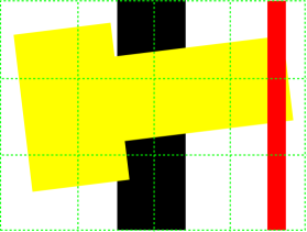
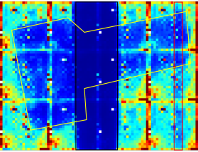
Figure 6.17: A schematic illustration (a) and a total intensity image (b) of the phantom object, obtained using the Manchester ERD HEXITEC detector. The phantom object consists of a cylinder of wax into which a bolt (yellow), a lead sheet (black) and a copper wire (red) are inserted.

Chapter 7 Conclusions

The EasyDD project is a first step in the right direction for the future development of computational tools to deal with the growing demand on data processing and analysis capabilities. Thanks to recent developments in the technology of radiation sources and data acquisition systems, this approach is an important endeavour in developing software that can cope with the massive and ever-increasing size of data collections that are generated in modern multi-tasking scientific experiments. EasyDD has already proved to be a crucial component within a number of key studies, e.g. [88] and [49]. Without the efficiency and speed of EasyDD, and without its effective strategies, such as the multi-batch processing approach, some of these studies may not have happened.

In the course of this PhD project, several experimental data collections on alumina-supported metal catalysts have been processed and analysed by the author using EasyDD. These include large data collections on molybdenum oxide, nickel nitrate calcination, nickel nitrate reduction, and nickel chloride based preparations. In the process, several chemical and crystallographic phases have been identified and mapped in terms of spatial location and time/temperature, thereby leading to important scientific implications. Amongst the many systems discussed in this thesis, the nickel chloride based system emerged as an outstanding example of what can be achieved in following its evolution (precursor, intermediates and final active phase) in terms of time, temperature, crystallite size and spatial distribution. Further, the high level of detail extracted enabled us to elucidate the overall evolving chemistry while also revealing new information on the physical state of the catalyst (crystallite size) and providing evidence and suggesting a mechanism for the inhomogeneity of crystallite size. This particular study stands out as a vivid example with which to demonstrate the capabilities and potential of these X-ray imaging and analysis techniques.

During this overall study a novel approach for processing and analysing massive data collections has emerged in which phase distribution pattern diagrams, combined with stack plots and standard diffraction patterns from powder diffraction databases, play a key role in summarising and presenting huge data sets in manageable form as an essential step to identifying phases and tracking the evolution of complex physical and chemical systems. As such, these developmental studies take diffraction-imaging capabilities way beyond those of previous landmark studies (e.g. Bleuet et al [20] and Espinosa-Alonso et al [49]) particularly for in situ and dynamic phase transformation studies. It is anticipated that these developments should have a significant future impact, at the scientific, technological and industrial level, within several fields of research such as catalysis, in operando studies, phase transformations, dynamic stress imaging of construction/biological materials etc. However, phase identification strategies for dynamic transformation studies of chemical and crystallographic systems still require further development as these systems are usually very complex and involve many phases.

Appendix A

Samples of EasyDD Code

In this appendix, we provide two snippets of EasyDD source code for two algorithms: back projection and channels alignment.

A.1 Back Projection Snippet

void MainWindow::backProjectTab()
{
    if(tabWidget->tabText(tabWidget->currentIndex()).contains("BP"))
    {
        QMessageBox::about(this, tr("Message"), "Back projection has been performed on this tab.
                                                 Use ’Back Projection Shift’.");
        return;
    }

    createBackProDialog();

    if(!bPOKFlag)
        return;

    if(allTabs.size()==0)
    {
        QMessageBox::about(this, tr("Message"), "There is no tab.");
        return;
    }

    if(bPStartAngle == bPStopAngle)
    {
        QMessageBox::about(this, tr("Message"), "Start and stop angles must be different.");
        return;
    }

    int tabIndex = this->tabWidget->currentIndex();
    int rotSide, traSide;

    if(bPRotTraFlag)
    {
        rotSide = allTabs[tabIndex].size();
        traSide  = allTabs[tabIndex][0]->Spectra.size();
    }
    else
    {
        traSide  = allTabs[tabIndex].size();
        rotSide = allTabs[tabIndex][0]->Spectra.size();
    }

    if(rotSide > traSide)
    {
        QMessageBox::about(this, tr("Message"), "The algorithm currently work only when rotation
                                                 side <= translation side.");
        return;
    }

    double bPStepAngle = (bPStopAngle-bPStartAngle)/(rotSide-1);
    QVector <double> anglesVec;

    if(bPReadAnglesFileFlag)
    {
        bPAnglesFileName = bPAnglesFileName.trimmed();
        QFile anglesFile(bPAnglesFileName);
        anglesFile.open(QIODevice::ReadOnly);
        QTextStream In(&anglesFile);

        if(!anglesFile.exists())
        {
            QMessageBox::about(this, tr("Message"), "The angles file ‘" + bPAnglesFileName +
                                                    "’ does not exist.");
            return;
        }

        QString ANG;

        while (!In.atEnd())
        {
            In >> ANG;
            ANG.simplified();
            if(ANG.isEmpty())
                continue;

            anglesVec.push_back(ANG.toDouble()*PI/180.0);
        }
    }
    else
    {
        for(int a=0; a<rotSide; ++a)
            anglesVec.push_back((bPStartAngle+a*bPStepAngle)*PI/180.0);
    }

    if(anglesVec.size() != rotSide)
    {
        QMessageBox::about(this, tr("Message"), "Number of angles not equal to side size.");
        return;
    }

    int nn2 = 2 * pow(2, ceil(log(1.0*traSide)/log(2.0)));
    Vec_IO_DP dataVec(nn2);
    QVector <double> Filt;

    if(bPFFTFlag == 1)
    {
        if(bPFilterTypeNum == 0)
        {
            QMessageBox::about(this, tr("Message"), "Filter should be chosen to proceed.");
            return;
        }
        else if(bPFilterTypeNum == 1)
        {
            for(int uu=0; uu<traSide; ++uu)
                Filt.push_back(fabs(sin(-PI+uu*(2*PI/traSide))));
        }
        else if(bPFilterTypeNum == 2)
        {
            for(int uu=0; uu<traSide; ++uu)
                Filt.push_back(fabs((-PI+uu*(2*PI/traSide))));
        }
    }

    allTables[tabIndex]->bPChanFlag = bPChannelsFlag;

    if(bPChannelsFlag == 1 || bPChannelsFlag == 2)
    {
        QVector < QVector <double> > filtPR;

        filtPR.resize(traSide);

        if(bPChannelsFlag == 1)
        {
            if(bPRotTraFlag)
            {
                for(int aa=0; aa<rotSide; ++aa)
                    for(int bb=0; bb<traSide; ++bb)
                        filtPR[aa].push_back(allTabs[tabIndex][aa]->Spectra[bb].Intensity);
            }
            else
            {
                for(int aa=0; aa<traSide; ++aa)
                    for(int bb=0; bb<rotSide; ++bb)
                        filtPR[bb].push_back(allTabs[tabIndex][aa]->Spectra[bb].Intensity);
            }
        }
        else if(bPChannelsFlag == 2)
        {
            if(bPStartChannel > bPEndChannel)
            {
                QMessageBox::about(this, tr("Message"), "Wrong channels range.");
                return;
            }

            if(bPEndChannel >= minMaxNumOfChannels[tabIndex].first)
            {
                QMessageBox::about(this, tr("Message"), "Wrong channels range.\nCommon channel
                    index range is 0-" + QString::number(minMaxNumOfChannels[tabIndex].first-1)
                    + ".");
                return;
            }

            if(bPRotTraFlag)
            {
                for(int aa=0; aa<rotSide; ++aa)
                    for(int bb=0; bb<traSide; ++bb)
                    {
                        double sum = 0.0;

                        for(int cc=bPStartChannel; cc<=bPEndChannel; ++cc)
                            sum += allTabs[tabIndex][aa]->Spectra[bb].dataPoints[cc].y();

                        filtPR[aa].push_back(sum);
                    }
            }
            else
            {
                for(int aa=0; aa<traSide; ++aa)
                    for(int bb=0; bb<rotSide; ++bb)
                    {
                        double sum = 0.0;

                        for(int cc=bPStartChannel; cc<=bPEndChannel; ++cc)
                            sum += allTabs[tabIndex][aa]->Spectra[bb].dataPoints[cc].y();

                        filtPR[bb].push_back(sum);
                    }
            }
        }

        if(bPFFTFlag == 1)
        {
            if(bPFftDftFlag)
            {
                for(int hh=0; hh<filtPR.size(); ++hh)
                {
                    int gg;
                    long int KK = 0;
                    for(gg=0; gg<filtPR[hh].size(); ++gg)
                    {
                        dataVec[KK]   = filtPR[hh][gg];
                        dataVec[KK+1] = 0.0;
                        KK += 2;
                    }
                    for(int tt=KK; tt<dataVec.size(); ++tt)
                        dataVec[tt] = 0.0;

                    fourierFFT(dataVec, 1);

                    KK = 0;
                    for(gg=0; gg<filtPR[hh].size(); ++gg)
                    {
                        dataVec[KK]   = dataVec[KK] * Filt[gg];
                        dataVec[KK+1] = dataVec[KK+1] * Filt[gg];
                        KK += 2;
                    }

                    fourierFFT(dataVec, -1);

                    KK = 0;
                    for(gg=0; gg<filtPR[hh].size(); ++gg)
                    {
                        filtPR[hh][gg] = dataVec[KK]/(nn2/2.0);
                        KK += 2;
                    }
                }
            }

            else
            {
                for(int hh=0; hh<filtPR.size(); ++hh)
                {
                    Vec_DP x1(filtPR[hh].size()), y1(filtPR[hh].size());
                    int gg;
                    for(gg=0; gg<filtPR[hh].size(); ++gg)
                    {
                        x1[gg]   = filtPR[hh][gg];
                        y1[gg]   = 0.0;
                    }

                    myFFT(1, filtPR[hh].size(), x1, y1);

                    for(gg=0; gg<filtPR[hh].size(); ++gg)
                    {
                        x1[gg]   = x1[gg] * Filt[gg];
                        y1[gg]   = y1[gg] * Filt[gg];
                    }

                    myFFT(-1, filtPR[hh].size(), x1, y1);

                    for(gg=0; gg<filtPR[hh].size(); ++gg)
                    {
                        filtPR[hh][gg] = x1[gg];
                    }
                }
            }
        }

        double midIndex = (1.0*traSide+1.0)/2.0;

        QVector < QVector <double> > BPI, xpr, ypr, filtIndex, BPIa;
        BPI.resize(traSide);
        xpr.resize(traSide);
        ypr.resize(traSide);
        filtIndex.resize(traSide);
        BPIa.resize(traSide);

        for(int b=0; b<BPI.size(); ++b)
            for(int c=0; c<BPI.size(); ++c)
            {
                BPI[b].push_back(0.0);
                xpr[b].push_back(1.0*c-midIndex+1.0);
                ypr[b].push_back(1.0*b-midIndex+1.0);
                filtIndex[b].push_back(0.0);
                BPIa[b].push_back(0.0);
            }

        QVector < int > tempI;
        QVector < QPair <int, int> > pairI;

        QVector < QVector < QPair <int, int> > >spota;
        QVector < QVector < int > >nfi;

        for(unsigned int mm = 0 ; mm < anglesVec.size() ; mm++)
        {
            QVector < QVector <int> > F;
            spota.push_back (pairI);
            nfi.push_back (tempI);

            for(unsigned int i = 0 ; i < traSide ; i++)
            {
                F.push_back(tempI);

                for(unsigned int j = 0 ; j < traSide ; j ++)
                {
                    double filtidx = floor(0.5+(midIndex+xpr[i][j]*sin(anglesVec[mm])-ypr[i][j]
                                           *cos(anglesVec[mm])));
                    F[i].push_back(filtidx);
                }
            }

            for(int k = 0  ; k < traSide; k ++)
            {
                for(unsigned int l = 0 ; l < traSide ; l ++)
                {
                    if (F[l][k] > 0 && F[l][k] <= traSide)
                    {
                        QPair <int,int> tem;
                        tem.first = l;
                        tem.second = k;

                        spota[mm].push_back(tem);
                        nfi[mm].push_back(F[l][k]-1);
                    }
                }
            }
        }

        for(unsigned int ii = 0  ; ii < rotSide ; ii++)
        {
            for(unsigned int jj = 0; jj <  spota[ii].size(); ++jj)
            {
                int r = spota[ii][jj].first;
                int c = spota[ii][jj].second;
                int ll = nfi[ii][jj];
                BPI[r][c] += filtPR[ii][ll];
            }
        }

        bPColorFlag[tabIndex] = 1;
        bPTabFlag[tabIndex] = 0;
        tempIntensityStore[tabIndex].resize(0);
        tempIntensityStore[tabIndex].resize(allTabs[tabIndex].size());

        for(int ss=0; ss<allTabs[tabIndex].size(); ++ss)
            for(int tt=0; tt<allTabs[tabIndex][ss]->Spectra.size(); ++tt)
                tempIntensityStore[tabIndex][ss].push_back(allTabs[tabIndex][ss]->
                                                            Spectra[tt].Intensity);

        if(traSide != rotSide)
            tabResize(tabIndex);

        for(int JJ=0; JJ<allTabs[tabIndex].size(); ++JJ)
            for(int KK=0; KK<allTabs[tabIndex][JJ]->Spectra.size(); ++KK)
            {
                if(allTabs[tabIndex][JJ]->Spectra[KK].dataPoints.size() == 0)
                {
                    allTabs[tabIndex][JJ]->Spectra[KK].dataPoints.resize
                                                        (minMaxNumOfChannels[tabIndex].first);
                    for(int MM=0; MM<minMaxNumOfChannels[tabIndex].first; ++MM)
                    {
                        allTabs[tabIndex][JJ]->Spectra[KK].dataPoints[MM].setX(0.0);
                        allTabs[tabIndex][JJ]->Spectra[KK].dataPoints[MM].setY(0.0);
                    }
                }
            }

        for(int aa=0; aa<BPI.size(); ++aa)
            for(int bb=0; bb<BPI[aa].size(); ++bb)
                allTabs[tabIndex][aa]->Spectra[bb].Intensity = BPI[aa][bb];

        QString newname = "BP" + QString::number(tabIndex+1);
        this->tabWidget->setTabText(tabIndex, newname);

        this->update();
    }

    else
    {
        if(bPComChanMesFlag)
        {
            bPComChanMesFlag = 0;
            QMessageBox::about(this, tr("Message"), "Back projection will be carried out for
                            common channels only, i.e. 0-"
                            + QString::number(minMaxNumOfChannels[tabIndex].first-1) + ".");
        }

        QVector < QVector < QVector <double> > > allVec;
        double midIndex = (1.0*traSide+1.0)/2.0;

        QVector < QVector <double> > xpr, ypr, filtIndex, BPIa;
        xpr.resize(traSide);
        ypr.resize(traSide);
        filtIndex.resize(traSide);
        BPIa.resize(traSide);

        for(int b=0; b<traSide; ++b)
            for(int c=0; c<traSide; ++c)
            {
                xpr[b].push_back(1.0*c-midIndex+1.0);
                ypr[b].push_back(1.0*b-midIndex+1.0);
                filtIndex[b].push_back(0.0);
                BPIa[b].push_back(0.0);
            }

        QVector < int > tempI;
        QVector < QPair <int, int> > pairI;

        QVector < QVector < QPair <int, int> > >spota;
        QVector < QVector < int > >nfi;

        for(unsigned int mm = 0 ; mm < anglesVec.size() ; mm++)
        {
            QVector < QVector <int> > F;
            spota.push_back (pairI);
            nfi.push_back (tempI);

            for(unsigned int i = 0 ; i < traSide ; i++)
            {
                F.push_back(tempI);
                for(unsigned int j = 0 ; j < traSide ; j ++)
                {
                    double filtidx = floor(0.5+(midIndex+xpr[i][j]*sin(anglesVec[mm])-ypr[i][j]
                                           *cos(anglesVec[mm])));
                    F[i].push_back(filtidx);
                }
            }

            for(int k = 0  ; k < traSide; k ++)
            {
                for(unsigned int l = 0 ; l < traSide ; l ++)
                {
                    if (F[l][k] > 0 && F[l][k] <= traSide)
                    {
                        QPair <int,int> tem;
                        tem.first = l;
                        tem.second = k;
                        spota[mm].push_back(tem);
                        nfi[mm].push_back(F[l][k]-1);
                    }
                }
            }
        }

        QProgressDialog progress(this);
        progress.setLabelText(tr("Performing back projection for each individual channel in
                                                    current tab.").arg("Tab Back Projection"));
        progress.setValue(0);
        progress.setRange(0, minMaxNumOfChannels[tabIndex].first-1);
        progress.show();

        unsigned long int count = 0;

        for(int oo=0; oo<minMaxNumOfChannels[tabIndex].first; ++oo)
        {
            progress.setValue(count);
            qApp->processEvents();
            if(progress.wasCanceled())
                return;
            count++;

            QVector < QVector <double> > BPI;
            BPI.resize(traSide);
            for(int dd=0; dd<traSide; ++dd)
                for(int zz=0; zz<traSide; ++zz)
                    BPI[dd].push_back(0.0);

            QVector < QVector <double> > filtPR;

            filtPR.resize(rotSide);

            if(bPRotTraFlag)
            {
                for(int aa=0; aa<rotSide; ++aa)
                    for(int bb=0; bb<traSide; ++bb)
                        filtPR[aa].push_back(allTabs[tabIndex][aa]->
                                        Spectra[bb].dataPoints[oo].y());
            }
            else
            {
                for(int aa=0; aa<traSide; ++aa)
                    for(int bb=0; bb<rotSide; ++bb)
                        filtPR[bb].push_back(allTabs[tabIndex][aa]->
                                        Spectra[bb].dataPoints[oo].y());
            }

            if(bPFFTFlag == 1)
            {
                if(bPFftDftFlag)
                {
                    for(int hh=0; hh<filtPR.size(); ++hh)
                    {
                        int gg;
                        long int KK = 0;
                        for(gg=0; gg<filtPR[hh].size(); ++gg)
                        {
                            dataVec[KK]   = filtPR[hh][gg];
                            dataVec[KK+1] = 0.0;
                            KK += 2;
                        }
                        for(int tt=KK; tt<dataVec.size(); ++tt)
                            dataVec[tt] = 0.0;

                        fourierFFT(dataVec, 1);

                        KK = 0;
                        for(gg=0; gg<filtPR[hh].size(); ++gg)
                        {
                            dataVec[KK]   = dataVec[KK] * Filt[gg];
                            dataVec[KK+1] = dataVec[KK+1] * Filt[gg];
                            KK += 2;
                        }

                        fourierFFT(dataVec, -1);

                        KK = 0;
                        for(gg=0; gg<filtPR[hh].size(); ++gg)
                        {
                            filtPR[hh][gg] = dataVec[KK]/(nn2/2.0);
                            KK += 2;
                        }
                    }
                }

                else
                {
                    for(int hh=0; hh<filtPR.size(); ++hh)
                    {
                        Vec_DP x1(filtPR[hh].size()), y1(filtPR[hh].size());
                        int gg;
                        for(gg=0; gg<filtPR[hh].size(); ++gg)
                        {
                            x1[gg]   = filtPR[hh][gg];
                            y1[gg]   = 0.0;
                        }

                        myFFT(1, filtPR[hh].size(), x1, y1);

                        for(gg=0; gg<filtPR[hh].size(); ++gg)
                        {
                            x1[gg]   = x1[gg] * Filt[gg];
                            y1[gg]   = y1[gg] * Filt[gg];
                        }

                        myFFT(-1, filtPR[hh].size(), x1, y1);

                        for(gg=0; gg<filtPR[hh].size(); ++gg)
                        {
                            filtPR[hh][gg] = x1[gg];
                        }
                    }
                }
            }

            for(unsigned int ii = 0  ; ii < rotSide ; ii++)
            {
                for(unsigned int jj = 0; jj <  spota[ii].size(); ++jj)
                {
                    int r = spota[ii][jj].first;
                    int c = spota[ii][jj].second;
                    int ll = nfi[ii][jj];
                    BPI[r][c] += filtPR[ii][ll];
                }
            }

            for(int x=0; x<BPI.size(); ++x)
            {
                for(int y=0; y<BPI[x].size(); ++y)
                {
                    BPI[x][y] = BPI[x][y]/(anglesVec.size()*1.0);
                }
            }

            allVec.push_back(BPI);
        }

        if(traSide != rotSide)
            tabResize(tabIndex);

        for(int ww=0; ww<traSide; ++ww)
            for(int xx=0; xx<traSide; ++xx)
            {
                allTabs[tabIndex][ww]->Spectra[xx].bPDataPoints = allTabs[tabIndex][ww]->
                                                                    Spectra[xx].dataPoints;
                allTabs[tabIndex][ww]->Spectra[xx].bPDataPoints.resize(allVec.size());

                for(int dd=0; dd<allVec.size(); ++dd)
                {
                    allTabs[tabIndex][ww]->Spectra[xx].bPDataPoints[dd].setX(dd);
                    allTabs[tabIndex][ww]->Spectra[xx].bPDataPoints[dd].setY(allVec[dd][ww][xx]);
                }
            }

        QString newname = "BP" + QString::number(tabIndex+1);
        this->tabWidget->setTabText(tabIndex, newname);
        backProjectTabShift();
    }
}

A.2 Channels Alignment Snippet

void MainWindow::alignChann()
{
    if(allTabs.size()==0)
    {
        QMessageBox::about(this, tr("Message"), "There is no tab.");
        return;
    }

    int inVoDi, a, b, c, d, e;
    int tabIdx = tabWidget->currentIndex();
    QVector < int > inVoDiVec;

    createAlignChanDialog();
    if(!alignOKDialogFlag)
        return;

    int parIdx = parIdxAlign;
    parIdx--;

    if(infFacAlign < 1 || infFacAlign > 50 || disNumAlign < 0
       || disNumAlign > allTabs[tabIdx][0]->Spectra.size()*infFacAlign/2 || parIdx < 0)
    {
        QMessageBox::about(this, tr("Message"), "Inappropriate input data. Operation aborted!");
        return;
    }

    for(a=0; a<allTabs[tabIdx].size(); ++a)
        for(b=0; b<allTabs[tabIdx][a]->Spectra.size(); ++b)
            if(!allTabs[tabIdx][a]->Spectra[b].isRefined
               || allTabs[tabIdx][a]->Spectra[b].refinedPars.size() < parIdxAlign)
            {
                QMessageBox::about(this, tr("Message"), "Not all voxels are refined OR parameter
                                                            index is wrong. Operation aborted!");
                return;
            }

    QProgressDialog progress(this);
    progress.setLabelText(tr("Aligning Channels").arg("Aligning"));
    progress.setValue(0);
    progress.show();

    clock_t startProgram(clock());

    QVector < QVector < double > > parVec;
    parVec.resize(allTabs[tabIdx].size());
    double temCO;

    for(a=0; a<allTabs[tabIdx].size(); ++a)
        for(b=0; b<allTabs[tabIdx][a]->Spectra.size(); ++b)
        {
            temCO = qMin(cutOffAlign, allTabs[tabIdx][a]->Spectra[b].refinedPars[parIdx]);
            parVec[a].push_back(temCO);
        }

    int newNumCols = 1+infFacAlign*(allTabs[tabIdx][0]->Spectra.size()-1);

    QVector < QVector < double > > chanInt;
    chanInt.resize(parVec.size());
    for(a=0; a<chanInt.size(); ++a)
        chanInt[a].resize(newNumCols);

    for(a=0; a<parVec.size(); ++a)
    {
        for(b=0; b<parVec[a].size()-1; ++b)
        {
            chanInt[a][b*infFacAlign] = parVec[a][b];
            for(c=(b*infFacAlign)+1; c<((b+1)*infFacAlign); ++c)
            {
                chanInt[a][c] = chanInt[a][b*infFacAlign] + (parVec[a][b+1] - parVec[a][b])
                                * (c-(b*infFacAlign)) / infFacAlign;
            }
        }
        chanInt[a].last() = parVec[a].last();
    }

    double center = chanInt[0].size() /2.0;
    double cenMas = 0;
    double sum = 0;

    for(b=0; b<chanInt[0].size(); ++b)
    {
        cenMas += b*chanInt[0][b];
        sum += chanInt[0][b];
    }

    cenMas /= sum;
    inVoDi = (int)(cenMas - center);

    inVoDiVec.push_back(-inVoDi);

    if(inVoDi > 0)
    {
        for(b=0; b<inVoDi; ++b)
        {
            double val = chanInt[0][0];
            chanInt[0].remove(0);
            chanInt[0].push_back(val);
        }
    }
    else
    {
        for(b=0; b<abs(inVoDi); ++b)
        {
            double val = chanInt[0].last();
            chanInt[0].remove(chanInt[0].size()-1);
            chanInt[0].prepend(val);
        }
    }

    for(a=1; a<chanInt.size(); ++a)
    {
        QVector < QPair < double, int> > LSVec;
        QVector < double > chanIntC;
        chanIntC.resize(chanInt[a].size());

        for(b=0; b<chanIntC.size(); ++b)
            chanIntC[b] = chanInt[a][b];

        for(b=0; b<disNumAlign; ++b)
        {
            double val = chanIntC[0];
            chanIntC.remove(0);
            chanIntC.push_back(val);
        }

        for(b=-disNumAlign; b<=disNumAlign; ++b)
        {
            double lsSum = 0;

            for(c=0; c<chanIntC.size(); ++c)
            {
                lsSum += (chanInt[0][c] - chanIntC[c]) * (chanInt[0][c] - chanIntC[c]);
            }

            QPair <double, int> lsIdx;
            lsIdx.first = lsSum;
            lsIdx.second = b;
            LSVec.push_back(lsIdx);

            double val = chanIntC.last();
            chanIntC.remove(chanIntC.size()-1);
            chanIntC.prepend(val);
        }

        qSort(LSVec.begin(), LSVec.end());
        inVoDi = LSVec[0].second;

        inVoDiVec.push_back(inVoDi);

        if(inVoDi < 0)
        {
            for(b=0; b<abs(inVoDi); ++b)
            {
                double val = chanInt[a][0];
                chanInt[a].remove(0);
                chanInt[a].push_back(val);
            }
        }
        else
        {
            for(b=0; b<inVoDi; ++b)
            {
                double val = chanInt[a].last();
                chanInt[a].remove(chanInt[a].size()-1);
                chanInt[a].prepend(val);
            }
        }
    }

    quint32 minNumChan = 9999999;
    long int maxNumChan = -9999999;

    for(b=0; b<allTabs[tabIdx].size(); ++b)
    {
        for(c=0; c<allTabs[tabIdx][b]->Spectra.size(); ++c)
        {
            minNumChan = (minNumChan < allTabs[tabIdx][b]->Spectra[c].dataPoints.size()) ?
                                minNumChan : allTabs[tabIdx][b]->Spectra[c].dataPoints.size();
            maxNumChan = (maxNumChan > allTabs[tabIdx][b]->Spectra[c].dataPoints.size()) ?
                                maxNumChan : allTabs[tabIdx][b]->Spectra[c].dataPoints.size();
        }
    }

    progress.setRange(0, minNumChan);
    quint16 count = 0;

    for(b=0; b<minNumChan; ++b)
    {
        progress.setValue(count);
        qApp->processEvents();
        if(progress.wasCanceled())
            return;
        count++;

        for(c=0; c<allTabs[tabIdx].size(); ++c)
        {
            for(d=0; d<allTabs[tabIdx][c]->Spectra.size()-1; ++d)
            {
                chanInt[c][d*infFacAlign] = allTabs[tabIdx][c]->Spectra[d].dataPoints[b].y();
                for(e=(d*infFacAlign)+1; e<((d+1)*infFacAlign); ++e)
                {
                    chanInt[c][e] = chanInt[c][d*infFacAlign]
                                    + (allTabs[tabIdx][c]->Spectra[d+1].dataPoints[b].y()
                                    - allTabs[tabIdx][c]->Spectra[d].dataPoints[b].y())
                                    * (e-(d*infFacAlign)) / infFacAlign;
                }
            }
            chanInt[c].last() = allTabs[tabIdx][c]->Spectra.last().dataPoints[b].y();
        }

        for(c=0; c<inVoDiVec.size(); ++c)
        {
            if(inVoDiVec[c] < 0)
            {
                for(d=0; d<abs(inVoDiVec[c]); ++d)
                {
                    double val = chanInt[c][0];
                    chanInt[c].remove(0);
                    chanInt[c].push_back(val);
                }
            }
            else
            {
                for(d=0; d<inVoDiVec[c]; ++d)
                {
                    double val = chanInt[c].last();
                    chanInt[c].remove(chanInt[c].size()-1);
                    chanInt[c].prepend(val);
                }
            }
        }

        for(c=0; c<allTabs[tabIdx].size(); ++c)
        {
            for(d=0; d<(allTabs[tabIdx][c]->Spectra.size()-1); ++d)
            {
                allTabs[tabIdx][c]->Spectra[d].dataPoints[b].setY(0);

                for(e=0; e<infFacAlign; ++e)
                    allTabs[tabIdx][c]->Spectra[d].dataPoints[b].ry() +=
                                                                    chanInt[c][(d*infFacAlign)+e];
            }
            allTabs[tabIdx][c]->Spectra.last().dataPoints[b].setY(chanInt[c].last());
        }
    }

    progress.setValue(minNumChan);

    double elapsedProgram = (double)(clock() - startProgram) / CLOCKS_PER_SEC;
    QMessageBox::about(this, tr("Message"), "Total time (sec): " +QString::number(elapsedProgram));
}