Rapid Thermalization by Baryon Injection in Gauge/Gravity Duality

Abstract

Using the AdS/CFT correspondence for strongly coupled gauge theories, we calculate thermalization of mesons caused by a time-dependent change of a baryon number chemical potential. On the gravity side, the thermalization corresponds to a horizon formation on the probe flavor brane in the AdS throat. Since heavy ion collisions are locally approximated by a sudden change of the baryon number chemical potential, we discuss implication of our results to RHIC and LHC experiments, to find a rough estimate of rather rapid thermalization time-scale $t_{\rm th}<1\,$[fm/c]. We also discuss universality of our analysis against varying gauge theories.

Introduction

The AdS/CFT correspondence Maldacena:1997re ; Gubser:1998bc ; Witten:1998qj , or more broadly, the gauge/gravity duality, is an extremely useful tool to study strongly coupled field theories. Recently, this correspondence has been applied to various field theory settings, and these applications open up many new correspondences between gravity to other branches of physics. Perhaps one of the most surprising things in the success of using gravity to study strongly coupled gauge theories is that it seems to work even for an explanation of heavy-ion collision experiment data at Brookhaven’s Relativistic Heavy Ion Collider (RHIC). In RHIC experiments Shuryak:2003xe ; Shuryak:2004cy , one of the big surprises was that a quark-gluon plasma (QGP) forms at a very early stage Heinz:2004pj just after the heavy ion collision, i.e. a rapid thermalization occurs. This obviously requires a theoretical explanation, but remains as a challenge, because this requires a calculation of the strongly coupled field theory in non-equilibrium process. In this letter, we study the thermalization in strongly coupled field theories by using the gauge/gravity duality.

The key idea is to approximate the heavy ion collision by a sudden change of a baryon-number chemical potential locally at the collision point. Using the AdS/CFT correspondence, we obtain strongly coupled gauge theory calculations for the thermalization, where a time-dependent confinement/deconfinement transition occurs due to a sudden change of the baryon-number chemical potential, with dynamical degrees of freedom changing from mesons to quark/gluon thermal plasma. We calculate a time-scale for that. Our strategy can be summarized briefly as follows; On the gravity side of the AdS/CFT correspondence, the change in the baryon chemical potential is encoded in how we throw in the baryonically-charged fundamental strings (F-strings) from the boundary to the bulk. Since the F-string endpoint is a source term for the gauge fields on the flavor brane in the AdS bulk, this provides a time-dependent gauge field configuration. This induces a time-dependent effective metric for the degrees of freedom on the flavor brane, which are mesons. As a result, this yields the emergence of an apparent horizon on the flavor brane, which signals, in the dual strongly coupled field theory, the “thermalization of mesons”, which we mean that the meson degrees of freedom change into quark and gluon degrees of freedom with thermal equilibrium.

Any computation of thermalization of mesons due to the injection of the baryon charge in strongly coupled gauge theories has never been proposed. We provide a generic framework for it in this paper. We also present computations at different gauge theories, and argue how universal the thermalization time-scale is. We also discuss its implication in strongly coupled gauge theories, which hopefully offers a path to realistic QCD. The observation of the flavor thermalization due to changes of external parameters (i.e., quantum quench) different from the baryon charge, was studied in Das:2010yw . Previous studies on holographic thermalization, for example in Janik:2006gp ; Chesler:2008hg ; Bhattacharyya:2009uu ; Chesler:2009cy ; Chesler:2010bi , discussed glueball sectors, while ours observes the meson sector thermalization. What we see is the thermalization on the probe flavor brane. Since the back-reaction is not taken in our setting, this thermalization is not at all related to the one of the glueball sectors.

In our framework, the only input is the function which represents how we throw in the baryonically charged F-strings. Therefore, we have small number of parameters, which includes a typical maximum value of the baryon density and the time-scale for changing the chemical potential. With collision parameters at RHIC, we obtain the thermalization time-scale as $t_{\rm th}<1\;[{\rm fm/c}]$. Actually this time-scale can be well compared with the known hydrodynamic simulation requirement $t_{\rm th}<2\;[{\rm fm/c}]$ discussed for example in Hirano:2001eu ; Kolb:2000fha ; Teaney:2001av ; Huovinen:2001xx ; Heinz:2002un . We also “predict” that heavy-ion collisions at CERN’s Large Hadron Collider (LHC) exhibit slightly smaller order of the time-scale for thermalization as $t_{\rm th}\lesssim{\cal{O}}\left(0.1\right)\;[{\rm fm/c}]$.

Let us make a few more comments about comparing our analysis with data. As we mention previously, we are discussing the time-scale of “thermalization of mesons”, which is the horizon formation on the probe brane only. In the real world experiments such as RHIC or LHC, thermalization should involve not only mesons but also glueballs, which corresponds to the black hole horizon formation in the bulk geometry, not only on the probe brane. Since we are not treating the glueball sectors, the “prediction” above in order to compare our analysis with the data is unfortunately not as accurate as it should be. Another worry for comparison with data is that we are discussing the large $N$ limit of gauge theories. Therefore, the reader should regard our analysis as just an indication of rapid thermalization of some sectors of the large $N$ gauge theories.

In the following, after solving the equations in the gravity side with a generic time-dependent baryon chemical potential, we compute the apparent horizon and the time-scale for the thermalization. The simplest example offered is ${\cal N}=4$ super Yang-Mills with ${\cal N}=2$ hypermultiplets as “quarks”. We conclude with the statement of the universality, by showing some variations of the setup, including quark masses and confining scales.

D3-D7 system with quark injection

The simplest set-up in AdS/CFT with quarks is the ${\cal N}=2$ supersymmetric massless QCD constructed by a D3-D7 system Karch:2002sh , where we consider the gravity back-reaction of only D3-branes and regard D7-brane as a prove flavor brane. We are interested in the dynamics of mesons and the deconfinement of quarks, which is totally encoded in the probe flavor D7-brane in the $AdS_{5}\times S^{5}$ geometry,

$$ds^{2}=\frac{r^{2}}{R^{2}}\eta_{\mu\nu}dx^{\mu}dx^{\nu}+\frac{R^{2}}{r^{2}}(d\rho^{2}\!+\!\rho^{2}d\Omega_{3}^{2}\!+\!dw_{5}^{2}\!+\!dw_{6}^{2}),{}$$ (1)

where $\rho^{2}\equiv w_{1}^{2}+w_{2}^{2}+w_{3}^{2}+w_{4}^{2}$ and $r^{2}\equiv\rho^{2}+w_{5}^{2}+w_{6}^{2}$. $R$ is the AdS radius defined by $R^{4}=4\pi g_{s}N_{c}\alpha^{\prime 2}$. The string coupling is related to the QCD coupling as $2\pi g_{s}\equiv g_{\rm QCD}^{2}$. The dynamics of the flavor D7-brane is determined by the D7-brane action

$$S=-\mu_{7}\int d^{8}\xi\sqrt{-\det\left(G_{ab}+2\pi\alpha^{\prime}F_{ab}\right)}\,,$$ (2)

where the D7-brane is at $w_{5}=0$ and are extended on the gauge theory directions $x^{\mu}$ ($\mu=0,1,2,3$), $\rho$, and $\Omega^{3}$. The fluctuations of gauge fields $A_{a}$ (or, scalar field $\eta\equiv w_{6}$) on the D7-brane corresponds to vector (or, scalar) mesons. For a concise review of the D3-D7 system and meson dynamics, see Erdmenger:2007cm . $G_{ab}$ is the induced metric on the D7-brane. The asymptotic $(\rho\to\infty)$ value of $\eta$ corresponds to the quark mass $m_{q}=\eta/2\pi\alpha^{\prime}$. For simplicity we first put it zero. This corresponding to a “marginal confinement” for the mesons on the flavor brane since it has only zero-sized horizon . The D7-brane tension is $\mu_{7}\equiv 1/(2\pi)^{7}g_{s}\alpha^{\prime 4}$.

In AdS/CFT, the response to the change in the baryon chemical potential is totally encoded in this D7-brane action. We will solve this gauge field for arbitrary time-dependent chemical potential.

As the chemical potential of our interest is homogeneous, we may turn on only the $F_{tr}$ component. With a redefinition of the AdS radial coordinate $z\equiv R^{2}/\rho$, the D7-brane action (2) is equivalent to a 1+1-dimensional Born-Infeld system in a curved background,

$$S=-\mu_{7}V_{3}{\rm Vol}(S^{3})\int\!dtdz\frac{R^{8}}{z^{5}}\sqrt{1-\frac{z^{4}}{R^{4}}(2\pi\alpha^{\prime})^{2}F_{tz}^{2}}\,,$$ (3)

where $V_{3}$ is the volume of $x^{1,2,3}$ space.

In the AdS/CFT dictionary, the static baryon chemical potential corresponds to $A_{t}(r=\infty)-A_{t}(r=0)$. This basically counts the number of electric charges located at the origin $r=0$. In order to change this number in a time-dependent manner, we need to consider an additional source term

$$\delta S=\mu_{7}V_{3}{\rm Vol}(S^{3})\int\!dtdz\left(A_{t}j^{t}+A_{z}j^{z}\right)\,,$$ (4)

which describes end-points of a fundamental string (electric charges) thrown in from the outside of the system, i.e., from the boundary into the bulk. See Fig. 1.

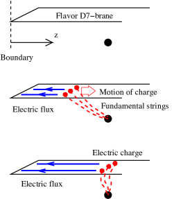
Figure 1: How the baryon charge density changes in time, as we throw-in fundamental strings from the boundary. Top figure: there is no baryon charge. Bottom figure: the static baryon (quark) charge is provided by the fundamental strings (dashed lines) connecting the probe D7-brane and the AdS horizon (black blob). The end points of the fundamental strings are electric charges (flavor charges) on the D7-brane. An electric flux (solid lines with arrows) emanates from those charges on the D7-brane. Middle figure: the flavor electric charges are thrown-in from the AdS boundary into the bulk. This specifies the time-dependent chemical potential. The electric flux is time-dependent. The big arrow denotes the motion of the electric charges on the D7-brane.

Since the geodesic of the fundamental string end-points is the light geodesics determined by the induced metric $G_{ab}$, and in the present case $G_{tt}=-G_{zz}$, it is just along a null vector $(v_{t},v_{z})=(1,-1)$. Therefore the source current is an arbitrary function of the variable $t-z$. With a current conservation relation, we obtain that $j^{t}=j^{z}$, and we take the arbitrary source function as $j^{t}=j^{z}=g^{\prime}(t-z)$. Given this source current $j$, the gauge field strength $F_{tz}$ is readily solved from the equations of motion on the D7-brane and we obtain

$$(2\pi\alpha^{\prime})F_{tz}=\frac{R^{2}z\;g(t-z)}{\sqrt{(2\pi\alpha^{\prime})^{2}R^{12}+z^{6}\left(g(t-z)\right)^{2}}}\,.$$ (5)

This is the gauge field solution which encodes the information of the time-dependent chemical potential given the source current $j^{t}=j^{z}=g^{\prime}(t-z)$.

The relation between $g$ and the chemical potential is linear. For the static case $g(t-z)=$ constant, the solution (5) is nothing but a conventional Born-Infeld solution on a D-brane. So we can compare the Born-Infeld charge $g$ with the fundamental string charge (which equals the quark number), following the techniques found in Callan:1997kz , to obtain

$$g(t)=(2/\pi)(2\pi\alpha^{\prime})^{4}\lambda\,n_{\rm B}(t)\,,$$ (6)

where the baryon number density is $n_{\rm B}=n_{\rm quark}/N_{c}$ at the boundary $z=0$. This determines the normalization of the baryon number, in the solution (5) of the D7-brane system.

Horizon formation on the flavor D7-brane

A time-dependent configuration on the D7-brane modifies the effective metric which the fluctuations on the D7-brane feels. A large field configuration creates a horizon of the metric on the D7-brane, which signals the thermalization in AdS/CFT. From the induced metric with the background gauge configuration (5), here we compute the location of an apparent horizon on the D7-brane .

Let us compute an effective metric which a scalar fluctuation $\eta$ feels, which is massless scalar meson like pion field. By expanding the D7-brane action (2) for small fluctuation $\delta\eta$ in the background solution $F_{tz}$ (5), to the quadratic order, we can obtain effective metric $\tilde{g}$ as:

$$S=-\!\!\int\!dtdzd^{3}x^{i}d^{3}\theta^{I}\;\frac{\sqrt{-\tilde{g}}}{2}\tilde{g}^{MN}\partial_{M}\delta\eta\partial_{N}\delta\eta+{{\cal O}(\delta\eta^{3})},\,$$ (7)

where $i=1,2,3$ is the spatial directions of our 3+1-dimensional space-time, and $\theta^{I}$ ($I=1,2,3$) is the angular variable on the $S^{3}$. $(M,N)$ shows the whole 7+1 directions on D7-branes, $(t,z,i,I)$. The effective metric $\tilde{g}$ can be obtained easily,

$$-\tilde{g}_{tt} = \tilde{g}_{zz}$$ (8)

$$= \mu_{7}^{1/3}R^{4/3}z^{-4/3}(1-z^{4}R^{-4}(2\pi\alpha^{\prime 2})F_{tz}^{2})^{5/6},$$

$$\tilde{g}_{ij} = \mu_{7}^{1/3}R^{4/3}z^{-4/3}(1-z^{4}R^{-4}(2\pi\alpha^{\prime 2})F_{tz}^{2})^{-1/6}\delta_{ij},$$

$$\tilde{g}_{IJ} = \mu_{7}^{1/3}R^{4/3}z^{2/3}(1-z^{4}R^{-4}(2\pi\alpha^{\prime 2})F_{tz}^{2})^{-1/6}G_{IJ},$$

where $G_{IJ}$ is the metric on the unit 3-sphere.

Given this effective metric, we will now determine the apparent horizon, which is defined locally as a surface whose area variation vanishes along the null rays which is normal to the surface. The surface area at an arbitrary point in given $(t,z)$ is

$$V_{\rm surface}\!\!\! = \!\!\!\int d^{3}x^{i}d^{3}\theta^{I}\sqrt{(\Pi_{i=1,2,3}\;\tilde{g}_{ii})(\Pi_{I=1,2,3}\;\tilde{g}_{II})}$$

$$= \!\!V_{3}{\rm Vol}(S^{3})\mu_{7}R^{4}z^{-1}(1-z^{4}R^{-4}(2\pi\alpha^{\prime 2})F_{tz}^{2})^{-1/2}.$$

The $(t,z)$ spacetime has a trivial null vector normal to the surface $(v^{t},v^{z})=(1,-1)$ since $\tilde{g}_{zz}=-\tilde{g}_{tt}$, so the constancy of the surface area variation along this null ray is

$$dV_{\rm surface}|_{dt=-dz}=0\,,$$ (10)

which yields

$$\left(\partial_{z}-\partial_{t}\right)\left[z^{2}(1-z^{4}R^{-4}(2\pi\alpha^{\prime 2})F_{tz}^{2})\right]=0.$$ (11)

Substituting the gauge field solution (5) to this, we obtain the following equation

$$(2\pi\alpha^{\prime})^{2}R^{12}-2z^{6}g^{2}+2z^{7}gg^{\prime}=0\,.$$ (12)

If this equation (12) admits a solution, it specifies where the apparent horizon on the D7-brane is formed.

Before we proceed, a few comments are in order. First, we are calculating the apparent horizon, not the event horizon on the flavor brane. Since apparent horizon is always inside the event horizon, as long as apparent horizon never disappears at finite time, we can regard the formation of the apparent horizon as a signal of the thermalization of system. However since the positions of the apparent horizon are time-dependent, it is difficult to extrapolate the thermodynamical information such as temperature, which is determined by the event horizon. On the other hand, the apparent horizons are defined locally without knowing the late time asymptotics, therefore it has a calculation simplicity. Secondary, we are using the Born-Infeld action on the flavor D7-brane to determine the effective metric for the various mesonic modes. This Born-Infeld form is crucial, since if we have used the Yang-Mills form for the D7’s degrees of freedom, the horizon would have not formed. The reason why we need the Born-Infeld form is due to the warping in the (1), which makes the effective string tension $\alpha^{\prime}$ finite, so it is not appropriate to replace the Born-Infeld action by the simple Yang-Mills form.

Thermalization time-scale order estimation

From (12), we can order-estimate the thermalization time-scale by a dimensional analysis without specifying the explicit form of the source function $g(t-z)$. We would like to consider the chemical potential change which mimics the heavy-ion collisions. The function $g(t-z)$ at the $AdS_{5}$ boundary $z=0$ is directly related to the time-dependent baryon number according to (6) as $g(t)=(2/\pi)(2\pi\alpha^{\prime})^{4}\lambda\,n_{\rm B}(t)$.

Suppose that $g(t-z)$ changes like trigonometric functions from zero to some maximal value during the time-scale $1/w$. This is like the situation where the chemical potential change locally by two baryonically-charged heavy ions approaching each other. Setting the maximal value of $g(t-z)$ as $g_{\rm max}$, we can order-estimate it as

$$g(\xi)\sim g_{\rm max}\,,\,g^{\prime}(\xi)\sim wg_{\rm max}\,.$$ (13)

Then, a dimensional analysis of (12) estimates the thermalization time-scale $t_{\rm th}$ as

$$t_{\rm th}\sim\left(\frac{(2\pi\alpha^{\prime})^{2}R^{12}}{g^{2}_{\rm max}}\right)^{1/6}\sim\left(\frac{\lambda}{n_{\rm B}^{2}}\right)^{1/6}\,,$$ (14)

if $t_{\rm th}w\lesssim 1$ is satisfied. Here $n_{\rm B}$ being the maximal baryon number density determined as $g_{max}=4(2\pi\alpha^{\prime})^{4}\lambda n_{\rm B}$. If $t_{\rm th}w\gg 1$ instead, then we obtain,

$$t_{\rm th}\sim\left(\frac{(2\pi\alpha^{\prime})^{2}R^{12}}{g^{2}_{\rm max}w}\right)^{1/7}\sim\left(\frac{\lambda}{n_{\rm B}^{2}w}\right)^{1/7}\,.$$ (15)

On the other hand, if $g(\xi)$ has an explicit $\xi$ dependence like a power-law behavior to approach its maximum, such as $g(\xi)\propto\xi^{n}$, with positive $n$, then

$$g(\xi)\sim g_{\rm max}(w\xi)^{n}\,,\,g^{\prime}(\xi)\sim wg_{\rm max}(w\xi)^{n-1}\,.$$ (16)

Again, a dimensional analysis yields,

$$t_{\rm th}\sim\left(\frac{(2\pi\alpha^{\prime})^{2}R^{12}}{g^{2}_{\rm max}w^{2n}}\right)^{1/{(6+2n)}}\sim\left(\frac{\lambda}{n_{\rm B}^{2}w^{2n}}\right)^{1/{(6+2n)}}\,.\quad$$ (17)

In summary, in terms of following parameters, inverse of the variation timescale of the baryon chemical potential $w$, ’t Hooft coupling $\lambda$, and the maximum baryon density $n_{\rm B}$, the thermalization time scale is written as

$$t_{\rm th}\sim\left(\frac{\lambda}{n_{\rm B}^{2}w^{k}}\right)^{1/{(6+k)}}\,.\quad$$ (18)

for given $k(\geq 0)$, which is determined by how we change the baryon number chemical potential. This is one of our main results.

In the following, we present two explicit examples of the source function $g(\xi)$ and show that both examples exhibit the generic behavior (18). The first example is for a baryonic matter formation, and the second is for baryons colliding and passing through each other.

Example I : Baryonic matter formation

To understand the time-scale in more detail, let us investigate a few explicit examples. The first example presented here mimics colliding baryons forming a baryonic matter. We start with zero baryon density $n_{\rm B}=0$ and then increase it linearly in time, for $0<t<1/w$. It reaches the maximum at $t=1/w$ and then it is kept constant. This is like two baryonically charged heavy-ion approaching each other, followed by a formation of a QGP gas with large baryon number. Setting $\xi\equiv t-z$, we arrange the function $g$ accordingly as

$$g(\xi)=\left\{\begin{array}[]{ll}0&\,(\xi<0)\\ g_{\rm max}\;w\,\xi&\,(0<\xi<1/w)\\ g_{\rm max}&\,(1/w<\xi)\end{array}\right.$$ (22)

With this choice of the time-dependent baryon number density, we can compute the location of the apparent horizon from (12). The results are,

$$t = \frac{3z}{2}+\frac{1}{2}\sqrt{z^{2}+\frac{\lambda}{z^{6}(2\pi)^{4}n_{\rm B}^{2}w^{2}}}\,$$ (23)

$$\mbox{(for $t<z+1/w$)}\,,\quad$$

and

$$z=\frac{1}{2\pi^{2/3}}\left(\frac{{\lambda}}{{n_{\rm B}^{2}}}\right)^{1/{6}}\,\mbox{(for $t>z+1/w$)}\,.$$ (24)

The curve (23) crosses with line $t=z+1/w$ at $z=z_{0}$ where $z_{0}$ satisfies

$$1-z_{0}w-\frac{{\lambda}}{64\pi^{4}n_{\rm B}^{2}z_{0}^{6}}=0\,,$$ (25)

and in the case $z_{0}w\ll 1$, $z=z_{0}$ coincides with the curve (24). These results are shown in Fig. 2.

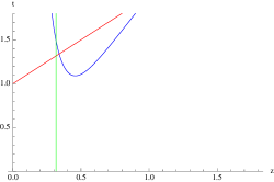
Figure 2: Locations of the apparent horizon in $z$-$t$ plane written in the unit of $1/w$ for the parameter is chosen such that $(\lambda/(2\pi n_{\rm B}^{2}))^{1/6}=1/w$. The blue, red, green curves/lines represent the curves/lines (23), $t=z+1/w$, and (24), respectively.

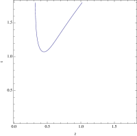
Figure 3: A numerical solution for the location of the apparent horizon for the source current given by $g(\xi)$ of (29), where the parameters and the unit are the same as Fig. 2. This is a smoothened version of the curve analytically determined in Fig. 2.

The slight discontinuity between curves (23) and (24) is simply due to a cusp of the input source function (22) at $\xi=1/w$. If we smoothen the source function (22), then the two curves (23) and (24) are connected smoothly. Just for a comparison, in Fig. 3 we also show the location curve for the apparent horizon for a smooth source current given by

$$g(\xi) = g_{\rm max}\;\frac{1}{2}\left(1+\tanh\left(2w\,\xi-1\right)\right)$$ (29)

$$= \left\{\begin{array}[]{ll}0&\,(w\xi\ll 1/2)\\ g_{\rm max}\;w\,\xi&\,(w\xi\sim 1/2)\\ g_{\rm max}&\,(w\xi\gg 1/2)\end{array}\right.$$

This Fig. 3 is well compared with Fig. 2.

The emergence of the horizon on the flavor D7-brane is seen by the boundary observer through a light propagation on the D7-brane. Suppose that the point A at $(t_{\rm A},z_{\rm A})$ in Fig. 4 gives the earliest delivery of the information of the apparent horizon. Due the fact that the light geodesic toward the $AdS_{5}$ boundary is again along the null vector $(v^{t},v^{z})=(1,-1)$, it is clear that the point A is determined by the curve (23) and its tangential outgoing null line, and it gives

$$t_{A}=c_{At}\left({\lambda}/{n_{B}^{2}w^{2}}\right)^{1/{8}}\,,\,z_{A}=c_{Az}\left({\lambda}/{n_{B}^{2}w^{2}}\right)^{1/{8}}\,,$$ (30)

where $c_{At}$ and $c_{Az}$ are order-one coefficients and given by $c_{\rm At}\equiv({11\sqrt{73}-13})^{1/2}/(48(2\pi)^{4}(5\sqrt{73}-31)^{3})^{1/8}\approx 0.88$ and $c_{\rm Az}\equiv\left({(5\sqrt{73}-31)}/{48(2\pi)^{4}}\right)^{1/8}\approx 0.33$. As a result, the thermalization time seen by the boundary observer is

$$t_{\rm th} = t_{\rm A}+z_{\rm A}=(c_{\rm At}\!+\!c_{\rm Az})\left(\frac{\lambda}{n_{B}^{2}w^{2}}\right)^{1/{8}}$$ (31)

$$\sim \left(\frac{{\lambda}}{{n_{\rm B}^{2}w^{2}}}\right)^{1/{8}}\,.$$

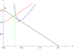
Figure 4: Earliest thermalization for the boundary observer occurs at point A, which is the tangential point between curve (23) (blue curve) and the light ray propagating toward boundary (black line). The boundary observer see the thermalization at point B. We choose the same paramete as Fig. 2.

On the other hand, it is also possible that the point C in Fig. 5 gives the earliest occasion, depending on the values of the parameters in the source function $g(\xi)$. This happens especially if

$$\frac{1}{w}\ll\left(\frac{\lambda}{n_{B}^{2}w^{2}}\right)^{1/8}\,.$$ (32)

In this case, similarly we can compute the thermalization time $t_{\rm th}$ as

$$t_{\rm th}=t_{\rm C}+z_{\rm C}\,,$$ (33)

with

$$t_{\rm C}=\frac{1}{w}+z_{\rm C}\,,\quad z_{\rm C}\equiv\frac{1}{2\pi^{2/3}}\left(\frac{{\lambda}}{{n_{B}^{2}}}\right)^{1/{6}}\,,$$ (34)

where $z_{\rm C}$ is given by the line (24). Therefore,

$$t_{\rm th} = 2z_{C}+\frac{1}{w}=\frac{1}{\pi^{2/3}}\left(\frac{{\lambda}}{{n_{B}^{2}}}\right)^{1/{6}}+\frac{1}{w}\,.$$ (35)

Due to the inequality (32), $1/w\ll 2z_{\rm C}$, this yields

$$t_{\rm th} \sim \left(\frac{{\lambda}}{{n_{B}^{2}}}\right)^{1/{6}}\,.$$ (36)

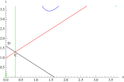
Figure 5: Curves for the parameter chosen $(\lambda/(2\pi n_{\rm B}^{2}))^{1/6}=(10)^{2/3}/w$, written in the unit of $1/w$. Thermalization occurs at point C, which is the crossing point between line (24) (green line) and the line $t=z+1/w$ (red line). From point C, the light ray is propagating toward boundary (black line), and the boundary observer see the thermalization at point D.

These results (31) and (36) are consistent with the order estimation (18) in the previous section.

Example II : Baryons passing through each other

Let us investigate another explicit example. This second example mimics baryons which first collide each other while then pass each other and leave. We start with zero baryon density $n_{\rm B}=0$ and then increase it linearly in time, for $0<t<1/w$. It reaches the maximum at $t=1/w$ and then decrease to zero again. This is like two baryonically charged heavy-ion approaching each other, and then they pass by due to the asymptotic freedom. Setting $\xi\equiv t-z$, we arrange the function $g$ accordingly as

$$g(\xi)=\left\{\begin{array}[]{ll}0&\,(\xi<0)\\ g_{\rm max}\;w\,\xi&\,(0<\xi<1/w)\\ g_{\rm max}\;(2-w\xi)&\,(1/w<\xi<2/w)\\ 0&\,(2/w<\xi)\\ \end{array}\right.$$ (41)

where $g_{\rm max}\equiv(2/\pi)(2\pi\alpha^{\prime})^{4}\lambda n_{\rm B}$ with $n_{\rm B}$ is the maximum baryon number density. Compared with an explicit example I, the location of the apparent horizon for $0<\xi<1/w$ is again given by the curve (23). On the other hand, for $1/w<\xi<2/w$, the curve is given by

$$t = \frac{2}{w}+\frac{3z}{2}-\frac{1}{2}\sqrt{z^{2}+\frac{\lambda}{z^{6}(2\pi)^{4}n_{\rm B}^{2}w^{2}}}\,$$ (42)

$$\mbox{(for $z+1/w<t<z+2/w$)}\,.\quad$$

Finally for $z+2/w<t$, (12) admits no solution, which means that there is no apparent horizon in this region. In Fig. 6, we plot these curves in the $z$-$t$ plane.

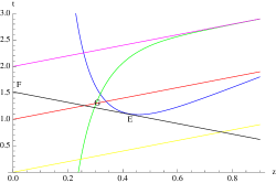
Figure 6: The curves (23) (blue) and (42) (green) and $t=z$ (yellow), $t=z+1/w$ (red), $t=z+2/w$ (magenta) and light ray (black) toward boundary which is tangential to (23) in the unit of $1/w$, where the parameter is chosen such that $(\lambda/(2\pi n_{\rm B}^{2}))^{1/6}=1/w$. It is clear for this parameter that the earliest apparent horizon is seen at point F, which is similar to point B in Fig. 4.

Similarly for a comparison, in Fig. 7 we show also the location curve for the apparent horizon for a smooth source which takes a Gaussian form as

$$g(\xi) = g_{\rm max}\;\exp\left(-\left(2w\right)^{2}\left(\xi-1/w\right)^{2}\right)\,.$$ (43)

This Fig. 7 is well compared with Fig. 6.

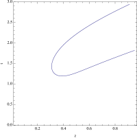
Figure 7: A numerical solution for the location of the apparent horizon written in the unit of $1/w$ for the source current which is given by $g(\xi)$ of (43), where the parameters are chosen as $(\lambda/(2\pi n_{\rm B}^{2}))^{1/6}=1/w$ and written in the unit of $1/w$. This is a smoothened version of the curve analytically determined in Fig. 6.

Similar to the explicit example I, from the curves (23) and (42), we can derive the thermalization time $t_{\rm th}$. From (23), we obtain again (31). From the other curve (42), the thermalization point is at the crossing of the green and the red lines in Fig. 6. The $z$ value of this crossing point, written as $z_{\rm G}$, is a solution of the equation

$$\frac{z_{\rm G}^{7}}{w}+\frac{z_{\rm G}^{6}}{w^{2}}-\frac{\lambda}{4(2\pi)^{4}n_{\rm B}^{2}w^{2}}=0\,.$$ (44)

With this, the thermalization time from the curve (42) is computed as $t_{\rm th}=2z_{\rm G}+1/w$. Therefore, from the two curves, we obtain the thermalization time as the earliest occasion among these two,

$$t_{\rm th} = \mbox{min}\left\{(c_{\rm At}+c_{\rm Az})\left(\frac{\lambda}{n_{\rm B}^{2}w^{2}}\right)^{1/8}\!\!\!\!\!\!,\;2z_{\rm G}+\frac{1}{w}\right\}.\quad$$ (45)

Note that in the case where the first term and the third term are well balanced in eq. (44), it gives,

$$z_{{\rm G}}\sim\left(\frac{\lambda}{n_{\rm B}^{2}w}\right)^{1/7}\,.$$ (46)

On the other hand, if the second term and the third term are balanced in eq. (44),

$$z_{{\rm G}}\sim\left(\frac{\lambda}{n_{\rm B}^{2}}\right)^{1/6}\,.$$ (47)

Therefore, if

$$1/w\lesssim t_{\rm th}$$ (48)

is satisfied, thermalization time-scale (45) becomes the lowest scale

$$t_{\rm th}\sim\mbox{min}_{\{k=0,1,2\}}\left\{\left(\frac{\lambda}{n_{\rm B}^{2}w^{k}}\right)^{1/(6+k)}\right\}\,.$$ (49)

Again this is consistent with the generic order estimation (18).

Comparison with experiments

We will later discuss the validity and the universality of our results in various other theories which are QCD-like theories. But before that, it is quite entertaining to substitute realistic values of the parameters and compare our results with the data, even though our setting is not realistic QCD at this point. For RHIC and LHC heavy ion collisions, the baryons are passing through each other, so we may approximate them by the example II above.

First, let us consider RHIC parameters. It is natural to assume that $n_{\rm B}$ is twice the standard nuclear density $n_{\rm N}$ times the Lorentz contraction factor $\gamma$, i.e., $n_{\rm B}\sim 2\gamma n_{\rm N}$, where $n_{\rm N}\sim 0.17[{\rm fm}]^{-3}$. In RHIC experiments, we have heavy ion Au-Au collisions with $A=197$. The Lorentz factor is given by the ratio between its energy scale $E=\sqrt{s_{NN}}/2\sim 100\;[\rm GeV]$ and the mass of Au $m_{\rm Au}$, therefore $\gamma=E/m_{Au}\sim 100$. On the other hand, at RHIC, the time scale $1/w$ should be given by the time scale of two nuclei passing by through their bodies, where two nuclei are propagating almost with the velocity of light. Therefore, $1/w$ is well approximated as $1/w\sim 2A^{1/3}/\gamma$ [fm/c], where $A$ is the nucleon number and $2A^{1/3}$ [fm] is the typical nuclear diameter. This gives $1/w\sim 0.1$ [fm/c].

With these inputs at hand, we obtain

$$\left(\frac{\lambda}{w^{2}n_{\rm B}^{2}}\right)^{1/8}\sim\left(\frac{A^{2/3}\lambda}{\gamma^{4}n_{\rm N}^{2}}\right)^{1/8}\sim 0.24\times\lambda^{1/8}\,[{\rm fm/c}]\,.$$ (50)

Similarly,

$$\left(\frac{\lambda}{wn_{\rm B}^{2}}\right)^{1/7} \sim \left(\frac{A^{1/3}\lambda}{\gamma^{3}n_{\rm N}^{2}}\right)^{1/7}\sim 0.30\times\lambda^{1/7}\,[{\rm fm/c}]\,,\quad$$ (51)

$$\left(\frac{\lambda}{n_{\rm B}^{2}}\right)^{1/6} \sim \left(\frac{\lambda}{\gamma^{2}n_{\rm N}^{2}}\right)^{1/6}\sim 0.39\times\lambda^{1/6}\,[{\rm fm/c}]\,.\quad$$ (52)

These are all bigger than $1/w\sim 0.1$, therefore approximately (48) is satisfied. In gauge/gravity duality, the ’tHooft coupling $\lambda=g_{\rm QCD}^{2}N_{c}$ is taken to be very large. However, since the power of $\lambda$ in $t_{\rm th}$ is small (less than one), $t_{\rm th}$ can not take a large value, even for large $\lambda$. Actually we use $\lambda\sim{\cal O}(10)$ which is often used in gauge/gravity duality for the spectrum comparison. In this case, the smallest of these are given by (50), though all the scale (50), (51), and (52) give the same order time-scale. Therefore we obtain the thermalization time-scale as

$$t_{\rm th}<1\,[{\rm fm/c}]\,.$$ (53)

It is interesting that this time-scale can be well compared with the known hydrodynamic simulation requirement $t_{\rm th}<2\;[{\rm fm/c}]$ Hirano:2001eu ; Kolb:2000fha ; Teaney:2001av ; Huovinen:2001xx ; Heinz:2002un . We found a rather rapid thermalization of mesons.

Our calculation can also gives a “prediction” for heavy ion collisions at LHC. In LHC where Pb-Pb ion collision experiments are on-going, the energy scale is bigger than RHIC as $\sqrt{s_{NN}}=2.7\;{\rm TeV}$ Collaboration:2010bu . The Lorentz factor is $\gamma=E/m_{Pb}\sim 1000$, due to the center of mass difference, and therefore, $\gamma$ is 10 times bigger in LHC than RHIC. Since $A\approx 200$ is almost the same, these give $1/w\sim 0.01\;[\rm fm/c]$. With these at hand, we can compute the thermalization time-scale. Due to the difference of Lorentz factor $\gamma$ compared with RHIC case in (50), (51), (52), the thermalization time-scale is suppressed furthermore in LHC, and we obtain

$$t_{\rm th}\lesssim{\cal{O}}\left(0.1\right)\;[{\rm fm/c}]\,.$$ (54)

Again, with $\lambda\sim{\cal O}(10)$ is used. (Due to the asymptotic freedom, $\lambda_{\rm LHC}<\lambda_{\rm RHIC}$, however the difference between $\lambda_{\rm RHIC}$ and $\lambda_{\rm LHC}$ is tiny therefore we can neglect this effect.) This (54) gives a significantly faster thermalization time-scale compared RHIC.

Thermalization for various modes

Given the calculation of the scalar meson thermalization in the massless ${\cal{N}}=2$ supersymmetric QCD, it is straightforward to extend the calculation of the thermalization for other degrees of freedom.

First, instead of the thermalization of the scalar meson $\eta$, let us consider that of vector mesons $A_{M}$. A similar computation leads to an effective metric of $A_{M}$ on the D7-brane, which gives the equation for the apparent horizon as

$$\left(\partial_{z}-\partial_{t}\right)\left[z^{4}(1-z^{4}R^{-4}(2\pi\alpha^{\prime 2})F_{tz}^{2})\right]=0\,.$$ (55)

This differs from (11) by just a power in the $z$ factor. According to this modification, the thermalization time is just $2^{1/3}$ times that of the scalar meson. Therefore the thermalization time-scale (53) is almost common in order, for various vector meson excitations on the flavor branes.

Next, we consider effects of the quark mass. The quark mass $m_{q}$ corresponds to the boundary location of the D7-brane, $\eta(z\!=\!0)=2\pi\alpha^{\prime}m_{\rm q}$. This shifts the D7-brane a bit. One can compute the full effect of this shift in our formalism, but we can give a naive estimate as follows. Noticing the fact that $\eta$ comes in the effective metric always as a combination $(R^{2}/z^{2}+\eta^{2}/R^{2})$ instead of just $R^{2}/z^{2}$, our computation presented here for $\eta=0$ is valid when

$$R^{2}/z^{2}\gg\eta^{2}/R^{2}.$$ (56)

Substituting the expression of $z$ by $z_{C}$ given by (34), we obtain

$$m_{\rm q}\ll(\sqrt{2}\lambda n_{\rm B}/\pi)^{1/3}.$$ (57)

Even without relying on the large ’tHooft coupling limit, this is generally satisfied for light three flavors, for the standard nuclear density. Therefore again we expect that the thermalization time-scale (53) is almost common in order, even for the various meson excitations with different flavors, such as up, down, and strange flavors.

Discussion on universality and real-world QCD

We saw that either in massless or massive ${\cal{N}}=2$ supersymmetric QCD, the calculations of the thermalization time-scales of the various meson modes are always given by (18). Given this, it is natural to ask to what extent our thermalization time-scale (18) holds for a larger variety of gauge theories. Since this question is related to a possible universality and also to real-world QCD-related problems, we shall discuss this question now.

First, note that even though our setting admits supersymmetry, it is also clear that we have never used the fermion properties for our thermalization calculations. Therefore we expect that our results are not much dependent on the supersymmetry.

Next, we shall see that, even with different background metrics, our thermalization timescale (18) is universal. We have used the AdS₅ metric (1), which represents the deconfined phase for the gluon sectors in the conformal ${\cal{N}}=4$ theory. However, the conformality of the gluon sector in the metric (1) is not important at all since our computations of thermalization reply only on the asymptotic part ($z<z_{0}$) of the induced metric, where $z_{0}$ is the point where apparent horizon emerge (such as $z_{\rm A},z_{\rm C},z_{\rm E},z_{\rm G}$ in our explicit examples I and II). Therefore we claim that our results hold for other theories where IR dynamics of gluons are significantly different from our theory. Even if we replace the metric (1) by some other non-conformal metric which does not admit a bulk horizon, such as a cut-off $AdS_{5}$ at $z\gtrsim z_{0}$, due to the fact that our calculations are insensitive to the IR regime of the geometry at $z\gtrsim z_{0}$, our conclusion is still valid. In this sense, we expect that our thermalization time-scale (18) is not only for the ${\cal{N}}=2$ theory, but rather it works for a broader category of non-conformal theories.

The scale $z_{0}\lesssim O(1)\;[\rm fm]$ in the example I and II we studied corresponds to the energy scale $\gtrsim{\cal O}(200)[\rm MeV]$. Therefore for any non-conformal theory which admits confinement/deconfinement transition for the gluon sectors at the scale smaller than $200[\rm MeV]$, our result (53) for the thermalization of mesons is expected to be valid. For the real-world QCD, confinement/deconfinement transition is $\sim 200[\rm MeV]$, which is the validity bound of our analysis, therefore it is expected that our results (53) also hold even for realistic QCD. However to confirm this, furthermore study is necessary.

Let us discuss confining gauge theories a bit more. On the gravity side, confinement is implemented as a deformation at the IR region ($z\sim\infty$) of the geometry. If we use successful hard-wall models in the bottom-up models of holographic QCD, which is with a cut-off of AdS₅ at IR $z>z_{0}$, then we obtain the same thermalization time-scale. One other example is a confining geometry made by D3-D(-1) system Liu:1999fc ; Kehagias:1999iy , which has the AdS₅ form at the UV region. In the solution the D(-1)’s (D-instantons) condense in the bulk and back-react to modify the IR $r\to 0$ region by emitting the dilaton $\phi$ as

$$ds^{2}=e^{\phi/2}\times\left({\rm AdS}_{5}\times{\rm S}^{5}\;\mbox{geometry}\right),\;e^{\phi}=1\!+\!\frac{q}{r^{4}}\,.$$ (58)

Here $ds^{2}$ is the metric in the string frame. In the UV $r\to\infty$, this reduces to the AdS metric (1), as advertized. The D(-1) charge $q$ (which is proportional to QCD instanton charge density) is related to the QCD string tension $\tau_{\rm QCD}$, as $q/R^{8}=\pi^{2}\lambda^{-1}\tau_{\rm QCD}^{2}$. This breaks the supersymmetries by half. The universality is valid if this factor $e^{\phi}$ may not significantly modify the asymptotic geometry around $z<z_{0}$, therefore we need to require $q<R^{8}z_{0}^{-4}$. With (34), this translates to a condition

$$\tau_{\rm QCD}<2^{5/3}\lambda^{1/6}n_{\rm B}^{2/3}.$$ (59)

Realistic parameters used in this paper show that $\tau_{\rm QCD}$ is at a comparable order with the right hand side, so this effect may modify the thermalization time-scale only slightly by an ${\cal O}(1)$ factor. Further study would be interesting for these.

Finally we comment on possible generalization of our approach for future works. We have conducted the calculations with the abelian Born-Infeld action, which treat a single flavor brane. In order to treat multi-flavors, we need to extend our analysis to non-abelian Born-Infeld action. It is interesting to generalize our study to non-abelian flavor branes and study the flavor dependence of the thermalization time-scale. Since our thermalization calculations are insensitive to the IR but are sensitive to the UV regime, if we consider totally different bulk geometries which do not approach the AdS₅ metric (1), our result (18) is not valid any more. It is quite interesting to generalize our approach to other theories where their UV geometries are different from ours, such as the holographic QCD model by D4-D8 on Witten’s geometry Witten:1998zw ; Sakai:2004cn , or Lifshitz type of geometries Kachru:2008yh for an application to condensed matter systems. We leave these studies for future works.

— Acknowledgment. K.H. would like to thank Tetsuo Hatsuda, Yoshitaka Hatta, Tetsufumi Hirano, Tadashi Takayanagi, and Koichi Yazaki for helpful comments and discussions. N.I. would like to thank Jorge Casalderrey-Solana, Sumit Das, and Kyriakos Papadodimas for helpful discussion and also for comments on the draft. N.I. also thanks RIKEN for its hospitality while visiting Japan. K.H. is partly supported by the Japan Ministry of Education, Culture, Sports, Science and Technology.

References

- (1) J. M. Maldacena, Adv. Theor. Math. Phys. 2, 231 (1998) [Int. J. Theor. Phys. 38, 1113 (1999)] [arXiv:hep-th/9711200].
- (2) S. S. Gubser, I. R. Klebanov and A. M. Polyakov, Phys. Lett. B 428, 105 (1998) [arXiv:hep-th/9802109].
- (3) E. Witten, Adv. Theor. Math. Phys. 2, 253 (1998) [arXiv:hep-th/9802150].
- (4) E. Shuryak, Prog. Part. Nucl. Phys. 53, 273 (2004) [arXiv:hep-ph/0312227].
- (5) E. V. Shuryak, Nucl. Phys. A 750, 64 (2005) [arXiv:hep-ph/0405066].
- (6) U. W. Heinz, AIP Conf. Proc. 739, 163 (2004) [arXiv:nucl-th/0407067].
- (7) S. R. Das, T. Nishioka, T. Takayanagi, JHEP 1007, 071 (2010). [arXiv:1005.3348 [hep-th]].
- (8) R. A. Janik and R. B. Peschanski, Phys. Rev. D 74, 046007 (2006) [arXiv:hep-th/0606149].
- (9) P. M. Chesler and L. G. Yaffe, Phys. Rev. Lett. 102, 211601 (2009) [arXiv:0812.2053 [hep-th]].
- (10) S. Bhattacharyya and S. Minwalla, JHEP 0909, 034 (2009) [arXiv:0904.0464 [hep-th]].
- (11) P. M. Chesler and L. G. Yaffe, Phys. Rev. D 82, 026006 (2010) [arXiv:0906.4426 [hep-th]].
- (12) P. M. Chesler and L. G. Yaffe, [arXiv:1011.3562 [hep-th]].
- (13) P. F. Kolb, P. Huovinen, U. W. Heinz and H. Heiselberg, Phys. Lett. B 500, 232 (2001) [arXiv:hep-ph/0012137].
- (14) T. Hirano, Phys. Rev. C65, 011901 (2001). [nucl-th/0108004].
- (15) P. Huovinen, arXiv:nucl-th/0108033.
- (16) D. Teaney, J. Lauret and E. V. Shuryak, arXiv:nucl-th/0110037.
- (17) U. W. Heinz and P. F. Kolb, arXiv:hep-ph/0204061.
- (18) A. Karch and E. Katz, JHEP 0206, 043 (2002) [arXiv:hep-th/0205236].
- (19) J. Erdmenger, N. Evans, I. Kirsch and E. Threlfall, Eur. Phys. J. A 35, 81 (2008) [arXiv:0711.4467 [hep-th]].
- (20) C. G. Callan, J. M. Maldacena, Nucl. Phys. B513, 198-212 (1998). [hep-th/9708147].
- (21) T. A. Collaboration, arXiv:1011.6182 [hep-ex].
- (22) H. Liu and A. A. Tseytlin, Nucl. Phys. B 553, 231 (1999) [arXiv:hep-th/9903091].
- (23) A. Kehagias and K. Sfetsos, Phys. Lett. B 456, 22 (1999) [arXiv:hep-th/9903109].
- (24) E. Witten, Adv. Theor. Math. Phys. 2, 505 (1998) [arXiv:hep-th/9803131].
- (25) T. Sakai and S. Sugimoto, Prog. Theor. Phys. 113, 843 (2005) [arXiv:hep-th/0412141].
- (26) S. Kachru, X. Liu and M. Mulligan, Phys. Rev. D 78, 106005 (2008) [arXiv:0808.1725 [hep-th]].