Unusual Yang-Lee edge singularity in the one-dimensional axial-next-to-nearest-neighbor Ising model.

Abstract

We show here for the one-dimensional spin-$1/2$ ANNNI (axial-next-to-nearest-neighbor-Ising) model in an external magnetic field that the linear density of Yang-Lee zeros may diverge with critical exponent $\sigma=-2/3$ at the Yang-Lee edge singularity. The necessary condition for this unusual behavior is the triple degeneracy of the transfer matrix eigenvalues. If this condition is absent we have the usual value $\sigma=-1/2$. Analogous results have been found in the literature in the spin-1 Blume-Emery-Griffths model and in the three-state Potts model in a magnetic field with two complex components. Our results support the universality of $\sigma=-2/3$ which might be a one-dimensional footprint of a tricritical version of the Yang-Lee-Edge singularity possibly present also in higher-dimensional spin models.

1 Introduction

In spin-$1/2$ models in an external magnetic field $H$, the partition function for finite number of spins is proportional to a polynomial on the variable $u=\exp(-2H/kT)$. Since polynomials are basically specified by their zeros, those zeros furnish all relevant physical information. Given that the partition function is a sum of exponentials (positive numbers) with positive coefficients, it is clear that we can only have zeros in the u-variable for complex magnetic fields. Such zeros for complex magnetic fields are called Yang-Lee zeros (YLZ) and are naturally studied on the complex-u plane as we do here. Their relevance in the study of phase transitions has been pointed out in 1952 by C. N. Yang and T. D. Lee, see [1].

In several spin models the YLZ tend, in the thermodynamic limit, to form continuous curves on the complex u-plane. In particular, it has been rigourously proved in [2] that all YLZ of the spin-$1/2$ Ising model, even before the thermodynamic limit, lie on the unit circle $|u|=1$. This circle theorem has been generalized, for example, to higher-spins Ising models [3] and to include other interacting terms [4]. As a rule, the zeros tend to leave the unit circle as the ferromagnetic (FM) Ising coupling $J$ becomes smaller as compared to other couplings. For more references see the review work [5]. At $T\leq T_{c}$ the YLZ tend to pinch the positive real axis on the complex-$u$ plane at the first-order and second-order phase transition points as we approach the thermodynamic limit. However, if $T>T_{c}$ they accumulate at the endpoints of the edges ($u_{E}=\exp(-2\beta H_{E})$) of the curves with a divergent linear density $\rho(u)\sim|u-u_{E}|^{\sigma}$ with $\sigma<0$.

As first noticed in [6] for the two-dimensional Ising model, the power-like behavior is independent of the temperature as long as $T>T_{c}$. The universality of the exponent $\sigma$ was explained in [7] as a result of a usual critical point described by a field theory with $i\,\Phi^{3}$ interaction vertex. The corresponding endpoints $u_{E}$ have been called Yang-Lee edge singularities (YLES). In $D=2$ dimensions, the use of conformal field theory [8] predicts $\sigma=-1/6$. This result has been verified for the Ising Model numerically [9, 10] and also experimentally from magnetization data [11].

According to arguments given in [12] one should have $\sigma=-1/2$ in one dimension. Notwithstanding, even in $D=1$ the exact position and density of the YLZ is not known analytically. One exception is the one-dimensional spin-$1/2$ Ising model. In this case the linear density was already known exactly [2] furnishing $\sigma=-1/2$. Numerical works have confirmed $\sigma=-1/2$ in several one-dimensional spin models [13, 14, 15, 16] including, see [17], the same model discussed here. An early exception is a special type of three-state Potts model [18]. In such model the spins are coupled with a magnetic field with two complex components. By fine-tuning the couplings of the model it has been obtained another type of YLES with $\sigma=-2/3$. More recently, inspired by the work of [16] we [19, 20] have shown that $\sigma=-2/3$ is not a peculiar feature of the special Potts model used in [18] but it is also present in the more familiar spin-1 Blume-Capel [21] and spin-1 Blume-Emery-Griffths (BEG) [22] models. Once again a fine-tuning of the couplings is required, which is typical of a tricritical phenomenon. In particular, we need to have a triple degeneracy of the transfer matrix eigenvalues. So far one has found this unusual value for $\sigma$ only in spin models with three states per site. Here we investigate the one-dimensional spin 1/2 axial-next-to-nearest-neighbor Ising (ANNNI) model, and confirm that the same unusual critical behavior also appears in models with two states per site and next-to-nearest-neighbor interaction. Our setup is based on the transfer matrix solution and the use of finite size scaling relations which are shown to be satisfied by the YLZ close to the unusual YLES.

2 The one-dimensional ANNNI model

The ANNNI model was introduced in [23], see also [24], as a simple model to describe spatially modulated periodic structures observed in magnetic and ferroelectric materials. In its higher-dimensional $(D>1)$ versions the model has interesting physical applications, see [25] for a review work. We concentrate here in its one-dimensional version as a simpler laboratory to investigate the existence of other types of Yang-Lee-Edge singularities. The energy and the partition function of the spin $1/2$ one-dimensional ANNNI model in an external magnetic field are given by:

$$E=-J\sum_{i}S_{i}S_{i+1}-K\sum_{i}S_{i}S_{i+2}-H\sum_{i}S_{i}$$ (1)

$$Z=\sum_{\{S_{i}\}}e^{-\beta E}$$ (2)

where $S_{i}=\pm 1$, $J$ and $K$ are coupling constants between nearest and next to nearest neighbor spins respectively and $H$ is the magnetic field. Usually the model is defined with $J>0$ (ferromagnetic or FM) and $K<0$ (anti-ferromagnetic or AFM) couplings. Here we start from a more general standpoint where $J$ and $K$ are arbitrary real numbers and the magnetic field $H$ can assume complex values. We use the notation:

$$c=e^{-\beta J},\quad d=e^{\beta K},\quad u=e^{2\beta H},\quad A=u+1/u=2\,\cosh(2\beta H).$$ (3)

The temperature is given in units of the nearest neighbor coupling, i.e., the range $0\leq T<\infty$ corresponds to $0\leq c\leq 1$ if $J>0$ or $c\geq 1$ if $J<0$. Likewise $-\infty<K\leq 0$ implies $0\leq d\leq 1$ while $0\leq K<\infty$ leads to $d\geq 1$. Here we use periodic boundary conditions, $S_{i}=S_{i+N}$. The partition function can be found via transfer matrix [17] :

$$Z_{N}={\textrm{\normalsize Tr}}\,\,T^{N}=\lambda_{1}^{N}+\lambda_{2}^{N}+\lambda_{3}^{N}+\lambda_{4}^{N}$$ (4)

where the $\lambda_{1}$, $\lambda_{2}$, $\lambda_{3}$ and $\lambda_{4}$ are the eigenvalues of the transfer matrix of the model and they can be determined by the characteristic equation:

$$\lambda^{4}-a_{3}\lambda^{3}+a_{2}\lambda^{2}-a_{1}\lambda+a_{0}=0$$ (5)

where

$$a_{0} = -\left(\frac{1}{d^{2}}-d^{2}\right)^{2}$$ (6)

$$a_{1} = d\,c\left(\frac{1}{d^{2}}-d^{2}\right)\sqrt{A+2}$$ (7)

$$a_{2} = d^{2}\left(\frac{1}{c^{2}}-c^{2}\right)$$ (8)

$$a_{3} = \frac{d}{c}\sqrt{A+2}$$ (9)

The ${\sf Z}_{2}$ symmetry $(H\to-H)$ of $Z_{N}$ is explicit in the factor $\sqrt{A+2}=e^{\beta\,H}+e^{-\beta\,H}$ present in $a_{1}$ and $a_{3}$. Notice that for $d=1$ we recover the spin-$1/2$ Ising model with only two eigenvalues.

3 $\sigma=-1/2$ and $\sigma=-2/3$ (Analytic approach)

The partition function $Z_{N}$ is proportional to a polynomial of degree $N$ in the “fugacity” $u$ (lattice gas interpretation). All relevant information about $Z_{N}$ is contained in its zeros $Z_{N}(u_{k})=0,k=1,2,...,N$. Due to the ${\sf Z}_{2}$ symmetry one half of the zeros is the inverse of the other half. For large number of spins we assume, see [26, 14], that the zeros are determined by imposing that at least two of the eigenvalues of the transfer matrix have the same absolute value which must be larger than the other two remaining ones, i.e.,

$$\lambda_{2}=e^{i\varphi}\lambda_{1}$$ (10)

$$|\lambda_{2}|=|\lambda_{1}|>|\lambda_{i}|,\quad i=3,4.$$ (11)

For large $N$ the contributions of $\lambda_{3}$ and $\lambda_{4}$ can be disregarded and the partition function becomes

$$Z_{N}\approx\lambda_{1}^{N}\left(1+e^{iN\varphi}\right)$$ (12)

Therefore the zeros are given by

$$\varphi_{k}=\left(2k-1\right)\frac{\pi}{N},\quad k=1,2,..,N.$$ (13)

The equations (5) and (10) imply

$$a_{3} = \lambda_{1}\left(1+e^{i\varphi}\right)+\lambda_{3}+\lambda_{4}$$ (14)

$$a_{2} = \lambda_{1}^{2}e^{i\varphi}+\lambda_{1}\left(\lambda_{3}+\lambda_{4}\right)\left(1+e^{i\varphi}\right)+\lambda_{3}\lambda_{4}$$ (15)

$$a_{1} = \lambda_{1}^{2}\left(\lambda_{3}+\lambda_{4}\right)e^{i\varphi}+\lambda_{1}\lambda_{3}\lambda_{4}\left(1+e^{i\varphi}\right)$$ (16)

$$a_{0} = \lambda_{1}^{2}\lambda_{3}\lambda_{4}e^{i\varphi}$$ (17)

In (14)-(17) we have four equations and four variables $\lambda_{1},\lambda_{3},\lambda_{4},\varphi$, eliminating $\lambda_{1}$, $\lambda_{3}$ and $\lambda_{4}$ we find an equation which depends only on $\varphi$:

$$F(A,c,d,\varphi) = 44\,a_{0}^{3}-7\,a_{1}^{4}+34\,a_{0}\,a_{1}^{2}\,a_{2}-28\,a_{0}^{2}\,a_{2}^{2}-2\,a_{1}^{2}\,a_{2}^{3}+6\,a_{0}\,a_{2}^{4}-40\,a_{0}^{2}\,a_{1}\,a_{3}+6\,a_{1}^{3}\,a_{2}\,a_{3}$$ (18)

$$- 24\,a_{0}\,a_{1}\,a_{2}^{2}\,a_{3}+34\,a_{0}^{2}\,a_{2}\,a_{3}^{2}+a_{1}^{2}\,a_{2}^{2}\,a_{3}^{2}-2\,a_{0}\,a_{2}^{3}\,a_{3}^{2}-2\,a_{1}^{3}\,a_{3}^{3}+6\,a_{0}\,a_{1}\,a_{2}\,a_{3}^{3}$$

$$- 7\,a_{0}^{2}\,a_{3}^{4}+2\,\left\{40\,a_{0}^{3}-a_{0}^{2}\,\left(24\,a_{2}^{2}+34\,a_{1}\,a_{3}-29\,a_{2}\,a_{3}^{2}+6\,a_{3}^{4}\right)\right.$$

$$+ \left.a_{0}\,\left[a_{1}^{2}\,\left(29\,a_{2}-2\,a_{3}^{2}\right)+a_{2}^{3}\,\left(4\,a_{2}-a_{3}^{2}\right)+a_{1}\,a_{2}\,a_{3}\,\left(-19\,a_{2}+5\,a_{3}^{2}\right)\right]\right.$$

$$- \left.a_{1}^{2}\,\left[6\,a_{1}^{2}+a_{2}^{3}+a_{1}\,\left(-5\,a_{2}\,a_{3}+a_{3}^{3}\right)\right]\right\}\,\cos(\varphi)+2\,\left\{31\,a_{0}^{3}+a_{1}^{3}\,\left(-3\,a_{1}+a_{2}\,a_{3}\right)\right.$$

$$+ \left.a_{0}\,\left[a_{2}^{4}+a_{1}^{2}\,\left(18\,a_{2}-a_{3}^{2}\right)+a_{1}\,a_{2}\,a_{3}\,\left(-8\,a_{2}+a_{3}^{2}\right)\right]-a_{0}^{2}\,\left(16\,a_{2}^{2}-18\,a_{2}\,a_{3}^{2}\right.\right.$$

$$+ \left.\left.3\,\left(8\,a_{1}\,a_{3}+a_{3}^{4}\right)\right]\right\}\,\cos(2\varphi)+\left(40\,a_{0}^{3}-2\,a_{1}^{4}\,+14\,a_{0}\,a_{1}^{2}\,a_{2}-16\,a_{0}^{2}\,a_{2}^{2}-26\,a_{0}^{2}\,a_{1}\,a_{3}\right.$$

$$- \left.2\,a_{0}\,a_{1}\,a_{2}^{2}\,a_{3}\,+14\,a_{0}^{2}\,a_{2}\,a_{3}^{2}\,-2\,a_{0}^{2}\,a_{3}^{4}\,\right)\cos(3\varphi)$$

$$+ \left(20\,a_{0}^{3}+2\,a_{0}\,a_{1}^{2}\,a_{2}-4\,a_{0}^{2}\,a_{2}^{2}\,-8\,a_{0}^{2}\,a_{1}\,a_{3}+2\,a_{0}^{2}\,a_{2}\,a_{3}^{2}\right)\cos(4\varphi)$$

$$+ \left(8\,a_{0}^{3}-2\,a_{0}^{2}\,a_{1}\,a_{3}\right)\cos(5\varphi)+2\,a_{0}^{3}\,\cos(6\varphi)=0$$

A similar expression has been derived before in [17] and analogous formulae for the one-dimensional spin-1 Blume-Capel and Blume-Emery-Griffiths models have appeared in [16] and [19] respectively. We interpret (18) as a cubic equation for $A=A(\varphi)$ such that when we plug it back in (5) we get two eigenvalues with the same absolute value according to (10). Equation (18) does not imply automatically the second condition (11). In practice we have to verify whether (11) holds for each of the three solutions $A_{i}(\varphi)\,,\,i=1,2,3$ of (18). At this point it is important to remark that, as its counterparts in [16, 17, 19], the equation (18) is symmetric under $\varphi\to-\varphi$. This symmetry is not accidental. It is a consequence of the permutation symmetry $\lambda_{1}\rightleftarrows\lambda_{2}$ hidden in (14)-(17). It becomes explicit when we perform $\left(\varphi\,,\,\lambda_{1}\right)\to\left(-\varphi\,,\,e^{i\,\varphi}\lambda_{1}\right)$. It is clear that after eliminating $\lambda_{1}\,,\,\lambda_{3}$ and $\lambda_{4}$ the resulting expression should be invariant under $\varphi\to-\varphi$. Such symmetry will play a key role in determining the points in the parameters space of the model where the unusual critical behavior $\sigma=-2/3$ shows up. Next we show how (18) can be combined with a finite size scaling relation to determine the exponent $\sigma$ analytically.

The closest zero $u_{1}[N]$ to the YLES $u_{1}[N\to\infty]$, for large $N$, should obey [27] the finite size scaling relation:

$$\Delta\,u_{1}(N)\equiv u_{1}[L]-u_{1}[\infty]=\frac{C_{1}}{L^{y_{h}}}=\frac{C_{1}}{N^{y_{h}}}\quad.$$ (19)

Where $y_{h}$ is the magnetic scaling exponent related to $\sigma$ via $\sigma=(D-y_{h})/y_{h}$. The constant $C_{1}$ is independent on the number of the spins $N$ and $N=L^{D}=L$.

It is known [28, 29] that the degeneracy of the two largest eigenvalues ($\lambda_{1}=\lambda_{2}$) of the transfer matrix signalizes a second-order phase transition. Therefore, the YLES occurs at $\varphi=0$. Thus, for large $N$, we can assume that the closest zero $u_{1}[N]$ is obtained from the smallest angle as $u_{1}[N]=u[\varphi=\varphi_{1}=\pi/N]$, see (13). We obtain $u(\varphi_{1})$ from the appropriate solution $A(\varphi_{1})$ of (18) via $u+1/u=A$. Expanding the result about $N\to\infty$, which amounts to know $A(\varphi)$ in the vicinity of $\varphi=0$, and comparing with (19) we determine $y_{h}$ and $\sigma$ analytically.

Although the exact solutions of the cubic equation (18) are cumbersome, they can be used to show that an expansion of $A(\varphi)$ about $\varphi=0$ contains only positive integer powers of $\varphi$. The key ingredient is that the coefficients of the cubic equation (18) are analytic functions of $\varphi$. Therefore we can write down the large $N$ expansion

$$A(\pi/N) = \left[A(0)+\varphi\left.\frac{dA}{d\varphi}\right|_{\varphi=0}+\frac{\varphi^{2}}{2!}\left.\frac{d^{2}A}{d\varphi^{2}}\right|_{\varphi=0}+\frac{\varphi^{3}}{3!}\left.\frac{d^{3}A}{d\varphi^{3}}\right|_{\varphi=0}+...\right]_{\varphi=\pi/N}$$ (20)

$$= A(0)+\frac{\pi}{N}\left.\frac{dA}{d\varphi}\right|_{\varphi=0}+\frac{\pi^{2}}{2N^{2}}\left.\frac{d^{2}A}{d\varphi^{2}}\right|_{\varphi=0}+\frac{\pi^{3}}{6N^{3}}\left.\frac{d^{3}A}{d\varphi^{3}}\right|_{\varphi=0}+...$$

Comparing (20) with (19), if the lowest non-vanishing derivative at $\varphi=0$ is $d^{j}A/d\varphi^{j}$ for some integer $j$ we have $y_{h}=j$ and $\sigma=(1-j)/j$. In order to find $j$, instead of using the complicated solutions of (18), it is more elucidative to take consecutive derivatives of (18) with respect to $\varphi$. From the first derivative of (18) we deduce, with help of (14)-(17), at $\varphi=0$ :

$$\left(\lambda_{1}-\lambda_{3}\right)^{3}\left(\lambda_{1}-\lambda_{4}\right)^{3}\left(\lambda_{3}-\lambda_{4}\right)^{2}\lambda_{1}\,d\left[c\left(\frac{1}{d^{2}}-d^{2}\right)+\frac{\lambda_{1}^{2}}{c}\right]\left.\frac{dA}{d\varphi}\right|_{\varphi=0}=0\quad.$$ (21)

Given that $\lambda_{1}=\lambda_{2}$ at $\varphi=0$, using $\lambda_{1}^{2}=c^{2}\left(d^{2}-\frac{1}{d^{2}}\right)$ in (5) we arrive at $\left(d^{4}-1\right)\left(c^{4}-1\right)=0$. Since $d$ and $c$ are non negative numbers, see (3), and $c=1$ corresponds to $T\to\infty$ while $d=1$ is the spin-$1/2$ Ising model for which $\sigma=-1/2$ is known exactly , we assume henceforth

$$\lambda_{1}^{2}\neq c^{2}\left(d^{2}-\frac{1}{d^{2}}\right)$$ (22)

Equations (21) and (22) tell us that

$$\left.\frac{dA}{d\varphi}\right|_{\varphi=0}=0\quad,\quad{\rm if}\,\,\lambda_{1}=\lambda_{2}\neq\lambda_{i}\,,\,i=3,4\quad{\rm and}\quad\lambda_{3}\neq\lambda_{4}$$ (23)

With help of (14)-(17) and (23), the second derivative of (18) at $\varphi=0$ furnishes:

$$\left(\lambda_{1}-\lambda_{3}\right)^{3}\left(\lambda_{1}-\lambda_{4}\right)^{3}\left(\lambda_{3}-\lambda_{4}\right)^{2}\lambda_{1}\left\{2d\left[c\left(\frac{1}{d^{2}}-d^{2}\right)+\frac{\lambda_{1}^{2}}{c}\right]\left.\frac{d^{2}A}{d\varphi^{2}}\right|_{\varphi=0}\right.$$

$$\left.+\lambda_{1}^{2}\left[(\lambda_{1}-\lambda_{3})(\lambda_{1}-\lambda_{4})\right]\right\}=0$$ (24)

From (22),(23) and (24) we have :

$$\left.\frac{d^{2}A}{d\varphi^{2}}\right|_{\varphi=0}\not=0\quad,{\rm if}\,\,\lambda_{1}=\lambda_{2}\neq\lambda_{i}\,,\,i=3,4\quad{\rm and}\quad\lambda_{3}\neq\lambda_{4}$$ (25)

In summary, from (23) and (25) we conclude that $y_{h}=2$ as long as we have neither a triple degeneracy of the transfer matrix eigenvalues nor two double degeneracies. Therefore, for the one-dimensional ANNNI model we show on general grounds that $\sigma=-1/2$, see also [17], except for the two mentioned special cases where a different critical behavior may appear in principle.

In the latter cases we have no information from (21) and (24). For triple degeneracy ($\lambda_{1}=\lambda_{2}=\lambda_{3}$) the coefficients in (5) must satisfy:

$$18\,a_{1}^{2}-14\,a_{1}a_{2}a_{3}+3\,a_{1}a_{3}^{3}-a_{2}^{2}a_{3}^{2}+4\,a_{2}^{3} = 2\,a_{0}\left(8\,a_{2}-3a_{3}^{2}\right)$$ (26)

$$9\left[12\left(a_{1}^{2}-a_{1}a_{2}a_{3}\right)+3\,a_{1}a_{3}^{3}-a_{2}^{2}a_{3}^{2}\right]+32\,a_{2}^{3} = 0$$ (27)

Working out (26) and (27) we arrive at :

$$d^{8}(8d^{4}-9)(1-c^{4})^{2}+108\,c^{4}(1-d^{4})^{2}=0\quad,$$ (28)

$$A=\frac{2(8\,d^{4}-7)}{8\,d^{4}-9}$$ (29)

Since both $c$ and $d$ are nonnegative real numbers, it is clear from (28) that we can only have triple degeneracy if $0<d<(9/8)^{1/4}$. The condition (28) is a second degree polynomial on $c^{4}$. Thus, there are only two possibilities for the temperature as a function of $d$:

$$c_{\pm}(d)=\left[\frac{\left(1-\frac{2}{3}d^{4}\right)^{3/2}\pm(d^{4}-1)}{\left(1-\frac{2}{3}d^{4}\right)^{3/2}\mp(d^{4}-1)}\right]^{1/4}$$ (30)

Notice, in agreement with (28), that $c_{-}(d)=1/c_{+}(d)$. In figure 1 we plot both $c_{\pm}(d^{4})$. They coalesce into $c_{-}=c_{+}=1$ ($T\to\infty$) at $d=1$. The function $c_{+}(d)$ diverges at $d=\left(9/8\right)^{1/4}$ while $c_{-}(d)$ vanishes at that point. By inserting $c_{+}(d)$ in the exact solutions of the cubic equation (18) and expanding the results about $\varphi=0$ we obtain:

$$A_{1}(\varphi) = \frac{2\,d^{12}-40\,{d^{8}}+117\,d^{4}-81}{d^{12}}-\frac{9\,\left(d^{4}-1\right)\,\left(2\,d^{4}-9\right)\,\left(2\,d^{4}-3\right)}{4\,d^{12}}\varphi^{2}$$ (31)

$$+ \frac{\left(d^{4}-1\right)\,\left\{3645+2\,d^{4}\,\left[-1944+d^{4}\,\left(297+64\,d^{4}\right)\right]\right\}}{216\,d^{12}}\varphi^{4}+{\cal O}(\varphi^{6})$$

$$A_{2}(\varphi) = \frac{2\,\left(8\,d^{4}-7\right)}{8\,d^{4}-9}+\frac{32\,i\left(d^{4}-1\right)\,{\sqrt{2\,d^{4}-3}}}{9\left(8\,d^{4}-9\right)}\varphi^{3}-\frac{8\,\left(d^{4}-1\right)}{27}\varphi^{4}$$ (32)

$$- \frac{2\,i\left(d^{4}-1\right)\,\left(8\,d^{4}-9\right)}{81{\sqrt{2\,d^{4}-3}}}\varphi^{5}+{\cal O}(\varphi^{6})$$

$$A_{3}(\varphi) = \frac{2\,\left(8\,d^{4}-7\right)}{8\,d^{4}-9}-\frac{32\,i\left(d^{4}-1\right)\,{\sqrt{2\,d^{4}-3}}}{9\left(8\,d^{4}-9\right)}\varphi^{3}-\frac{8\,\left(d^{4}-1\right)}{27}\varphi^{4}$$ (33)

$$+ \frac{2\,i\left(d^{4}-1\right)\,\left(8\,d^{4}-9\right)}{81{\sqrt{2\,d^{4}-3}}}\varphi^{5}+{\cal O}(\varphi^{6})$$

The solutions $A_{2}$ and $A_{3}$ are interchanged under the symmetry $\varphi\to-\varphi$ of (18) while $A_{1}$ is invariant.

It turns out that only $A_{2}(\varphi)$ and $A_{3}(\varphi)$ satisfy, at $\varphi=0$, the triple degeneracy condition (29). Indeed, substituting $c=c_{+}(d)$ and $A=A_{i}(\varphi)$ in (5) one obtains the four transfer matrix eigenvalues $\lambda_{\alpha}=\lambda_{\alpha}(\varphi)\,,\,\alpha=1,2,3,4$ for each solution $A=A_{i}(\varphi)\,,\,i=1,2,3$. We have checked numerically for several values of $d$ in the range $0<d<(9/8)^{1/4}$ that $A=A_{1}(\varphi)$ only leads to double degeneracy $\lambda_{1}=\lambda_{2}$ at $\varphi=0$. Besides, it is such that $|\lambda_{1}(\varphi)|=|\lambda_{2}(\varphi)|<|\lambda_{i}(\varphi)|\,,\,i=3,4$ in the neighborhood of $\varphi=0$. So, $A_{1}(0)$ does not correspond to a true edge singularity. On the other hand, the function $A_{3}(\varphi)$, though it leads to triple degeneracy $\lambda_{1}=\lambda_{2}=\lambda_{3}$ at $\varphi=0$, it is such that $|\lambda_{1}(\varphi)|=|\lambda_{2}(\varphi)|$ is not the largest absolute value in the vicinity of $\varphi=0$. Thus, we do not have partition function zeros for $A=A_{3}(\varphi)$. For $A=A_{2}(\varphi)$ we have checked that $\lambda_{1}=\lambda_{2}=\lambda_{3}$ at $\varphi=0$ and more importantly $|\lambda_{1}(\varphi)|=|\lambda_{2}(\varphi)|>|\lambda_{i}(\varphi)|\,,\,i=3,4\,$ which confirms that we do have Yang-Lee zeros approaching the YLES $A_{2}(0)$ for $A=A_{2}(\varphi)$.

From the above discussion and (32) we conclude that for the fine-tuning $c=c_{+}(d)$ we assure a different critical behavior with $j=3=y_{h}$ ($\sigma=-2/3$) for the density of Yang-Lee zeros at the YLES.

Regarding the second possibility $c=c_{-}(d)=1/c_{+}(d)$ it is possible to show that in this case we have the usual result $j=2=y_{h}$ ($\sigma=-1/2$). Indeed, it can be checked analytically that the cubic equation (18) is symmetric under $c\to 1/c$. However, there is no such symmetry in (5). If we plug $c=c_{-}(d)$ and $A_{1}(\varphi)$ in (5), it turns out that $\lambda_{1}=\lambda_{2}$ at $\varphi=0$ and $|\lambda_{1}(\varphi)|=|\lambda_{2}(\varphi)|>|\lambda_{i}(\varphi)|\,,\,i=3,4$ in the neighborhood of $\varphi=0$. So we have a true YLES with, see (31), $j=2=y_{h}$ ($\sigma=-1/2$). The other functions $A_{2}(\varphi)$ and $A_{3}(\varphi)$ lead to $\lambda_{1}=\lambda_{2}=\lambda_{3}$ at $\varphi=0$ but $|\lambda_{1}(\varphi)|=|\lambda_{2}(\varphi)|$ is not the largest absolute value about $\varphi=0$. So, we do not have Yang-Lee zeros in those cases. Analogously, the case of two double degeneracies $\lambda_{1}=\lambda_{2}\neq\lambda_{3}=\lambda_{4}$ leads only to $\sigma=-1/2$.

We see from (29), which gives the location of the YLES in the triply degenerated case, that we can only have $\sigma=-2/3$ either for zeros lying on the unit circle ($-2\leq A\leq 2$), with $0\leq d\leq 1$ (AFM coupling $K<0$), or on the negative real axis ($A<-2$) which requires $1<d<(9/8)^{1/4}$ (FM coupling $K>0$). In the first case $0\leq c_{+}(d)\leq 1$ (FM coupling $J>0$) while in the second one $c>1$ (AFM coupling $J<0$). Therefore, the unusual critical behavior $\sigma=-2/3$ only occurs for couplings $J$ and $K$ of opposite nature.

As a final remark we note from (32) that $j\neq 3$ if $d^{4}=3/2$, which coincides precisely, using $c=c_{+}(d)$, with the quadruple degeneracy of the eigenvalues $\lambda_{1}=\lambda_{2}=\lambda_{3}=\lambda_{4}$. However, in this case $c_{+}$ becomes complex and it will be neglected here. Anyway, this is an indication that different values for $\sigma$ are associated with multiple degeneracies of the transfer matrix eigenvalues.

In the next section our analytic results are confirmed by numerical calculations of the Yang-Lee zeros.

4 Numerical results

Comparing the FSS relation (19) for two rings of sizes $N_{a}$ and $N_{a+1}$ we derive a numerical estimate for $y_{h}$

$$y_{h}=-\left[\ln\frac{N_{a+1}}{N_{a}}\right]^{-1}\ln\left[\frac{\Delta u_{1}(N_{a+1})}{\Delta u_{1}(N_{a})}\right]\quad.$$ (34)

Where either the imaginary or the real part of $\Delta u_{1}(N)$ can be used. In the case of triple degeneracy, the YLES $u_{1}^{\pm}(\infty)=u_{E}^{\pm}$ are known exactly by inverting the relation $u_{E}+1/u_{E}=A_{E}$ where $A_{E}$ is given in (29) for each value of $d$. Since $A_{E}\in\Re$ it follows that $u_{E}^{-}=(u_{E}^{+})^{*}$. So we choose $u_{E}=u_{E}^{+}$ without loss of generality.

We also consider another finite size scaling relation [27, 30] for the linear density of zeros close to the YLES:

$$\rho(L)=C_{2}\,L^{y_{h}-D}=C_{2}N^{y_{h}-1}$$ (35)

where $C_{2}$ is a constant independent on the number of the spins $N$ while $N=L^{D}=L$. Analogous to (34) we can derive from (35):

$$y_{h}=1+\left[\ln\frac{N_{a+1}}{N_{a}}\right]^{-1}\ln\left[\frac{\rho(N_{a+1})}{\rho(N_{a})}\right]$$ (36)

The scaling exponents obtained from (34) and (36) will be called respectively $y_{h}^{E}$ and $y_{h}^{\rho}$. More specifically, we use $y_{h}^{E,Re}$ and $y_{h}^{E,Im}$ according to the use of real or imaginary parts of $\Delta\,u_{1}(N)$. We stress that (34) and (36) furnish independent numerical estimates for $y_{h}$, since $\rho(N)=1/\left(N|u_{1}-u_{2}|\right)$ depends upon the first and second closest zeros, $u_{1}\,,\,u_{2}$ to the YLES while $y_{h}^{E}$ depends only upon the first one. Later on, we will extrapolate the finite size results (34) and (36) for $N\to\infty$ via BST (Burlish-Stoer) extrapolation algorithm [31, 32].

The partition function zeros for a ring with $N$ sites (spins) are obtained numerically with help of the software Mathematica from an analytic expression for $Z_{N}$. Even for one-dimensional spin models there are no analytic expressions for the Yang-Lee zeros in general. In order to save computer time, instead of using the analytic solution for $Z_{N}$ given in (4) in terms of the transfer matrix eigenvalues or in terms of the trace of powers of the transfer matrix as in ${\rm Tr}\,T^{N}$, we use an alternative exact expression derived in [20] for any spin model which can be solved via a finite transfer matrix. Namely, since $\lambda_{i}\,,\,i=1,2,3,4$ are solutions of the secular equation $P_{4}(\lambda)\equiv\lambda^{4}-a_{3}\lambda^{3}+a_{2}\lambda^{2}-a_{1}\lambda+a_{0}=0$, we have shown, formula (11) of [20], that (4) can be identified with

$$Z_{N}=-N\left\{\ln\left[g^{4}P_{4}(1/g)\right]\right\}_{g^{N}}=-N\left[\ln\left(1-a_{3}g+a_{2}g^{2}-a_{1}g^{3}+a_{0}g^{4}\right)\right]_{g^{N}}\quad,$$ (37)

where $g$ is an arbitrary real variable (power counting parameter) and $\left[f(g)\right]_{g^{N}}$ stands for the coefficient of the term of power $g^{N}$ in the Taylor series of $f(g)$ about $g=0$. For the lowest powers $N=1,2,3$ the reader can easily check, with help of (14)-(17) at $\varphi=0$, that (37) indeed reproduces the transfer matrix solution (4).

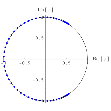
(a)

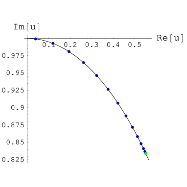
(b)

Figure 3: (Color online) Yang-Lee zeros and half of the Yang-Lee edge singularities (green (light gray) dot) for $N=60$ spins at $d\approx 0.8680$ and $c=0.5$ (triple degeneracy point)

At each value of $d$, the expression $c_{+}(d)$, see (30), furnishes the corresponding fine-tuned temperature for triple degeneracy,. We can also invert $c_{+}(d)$ and obtain $d$ for each given value of $c$. If, for instance, we choose $c=0.5$, the inversion of $c_{+}(d)$ leads to $d\approx 0.8680$. We have displayed in figures 2-4 the YLZ and half of the corresponding YLES (with positive imaginary part) for $d\approx 0.8680$ and $c=0.48\,,\,0.50\,,\,0.52$. It turns out that the triple degeneracy point is a turning point after which each edge bifurcates into two new ones. Right above the triple degeneracy point ($c>0.50$) we have checked (not shown here) that at the endpoint of each of the two new edges, figure 4(b), the critical exponent is the usual one $y_{h}=2$ ($\sigma=-1/2$) while right before ($c<0.50$) we have a crossover behavior flowing from $y_{h}=2$ to $y_{h}=3$ as we approach $c=0.50$ from below.

At the triple degeneracy point we have made a detailed analysis of the scaling behavior of the zeros in the neighborhood of the YLES which is located, see (29) at $d\approx 0.8680$, at $A_{E}\approx 1.1031$ ($u_{E}\approx 0.5516\pm 0.8341\,i$). In this case all Yang-Lee zeros lie on the unit circle, see figure 3.

The log-log fits in figures 5(a) and 5(b) confirm the FSS relations (19) and (35). They furnish the estimates $y_{h}^{E}=2.9960$ (using the real pat of the zeros) and $y_{h}^{\rho}=2.9866$.

In table (1) we present the sequences $y_{h}(N_{a})$ obtained from formulae (34) and (36). In the last line we have extrapolated our finite size results $N\to\infty$ by using the BST [31, 32] algorithm with $\omega=1$. This algorithm approximates the original sequence $y_{h}(N_{a})$ by another sequence of ratios of polynomials with faster convergence. The BST approach depends upon the real free parameter $\omega$: $y_{h}(N)=y_{h}(\infty)+\frac{A_{1}}{N^{\omega}}+\frac{A_{2}}{N^{2\omega}}+...$ where $A_{1},A_{2},\cdots$ are $N$-independent constants. We plot the extrapolated quantity $y_{h}(\infty)$ for $0.1\leq\omega\leq 3.0$ altogether with their error bars in figure 6. The error bar corresponds to twice the difference between the values of $y_{h}$ obtained at the step before the last one in the extrapolating sequence. In table (1) we have chosen $\omega=1$ because it provides a more stable result, i.e., $\frac{dy_{h}}{dw}=0$. Clearly from table (1) and figures 5 and 6 we have a result very close to $y_{h}=3$ ($\sigma=-2/3$) at the triple degeneracy point. We have also checked numerically other couples of values for $(c,d)$ satisfying the triple degeneracy condition $c=c_{+}(d)$. The BST extrapolated results for $y_{h}$ are very similar as well as their error bars. Some caution is needed when the edges are nearly horizontal (vertical) lines. In those cases the smallest error bars for $y_{h}^{E}$ are obtained by the use of the real (imaginary) part of the first zero respectively.

5 Conclusion

Usually, in one-dimensional spin models, the linear density of partition function zeros diverges with a critical exponent $\sigma=-1/2$ at edge singularities. The universality of $\sigma$ is known for a long time [6, 7, 12] and checked explicitly in $D=1$ in several models, see e.g. [13, 14, 15, 16, 17]. However, in the works [18, 19, 20] one has found another critical behavior ($\sigma=-2/3$). The models investigated in [18, 19, 20] have three-state per site and only nearest-neighbor interaction. Here we have shown that $\sigma=-2/3$ also appears in the one-dimensional spin-$1/2$ ANNNI model which contains a next-to-nearest-neighbor interaction and only two states per site. Our results support the universality of $\sigma=-2/3$. As in [19, 20], the triple degeneracy of the transfer matrix (TM) eigenvalues is necessary to evade the well known result $\sigma=-1/2$. Such condition requires a fine-tuning of the couplings of the model which explains why the authors of [17] have only found $\sigma=-1/2$ for the same model treated here. So, rather than the number of states per site, the important point is the dimension of the TM and the number of the free parameters of the model to be fine-tuned.

The above argument signalizes that the same phenomenon might occur in higher-dimensional spin models under special circumstances, since for $D>1$ the number of eigenvalues of the TM increases with the size of the lattice. In particular, one could speculate that this phenomenon might be behind the sudden drop from $\sigma=-0.15(2)$ down to $\sigma=-0.365$ as reported in [11], similarly to the drop from $\sigma=-1/2$ to $\sigma=-2/3$. In [11] one obtains the linear density of Yang-Lee zeros for the two-dimensional Ising model, above the critical temperature, indirectly from a function that fits the experimental magnetization data from a sample of FeCl₂. The $2D$-Ising model works as a prototype for FeCl₂ in some temperature range. As shown already in [6] the discontinuity of the magnetization across the curve of zeros furnishes their density. So one has indirect access to $\sigma$ experimentally.

Another interesting point is that the triple degeneracy condition $c=c_{+}(d)$ as given in (30) defines a transition point between two different loci of Yang-Lee zeros. For $c<c_{+}(d)$ we have an arc of the unit circle with two edges while for $c>c_{+}(d)$ each edge bifurcates into two new edges with some fraction of zeros leaving the unit circle, see figure 2 and figure 4. Our figure 4 is similar to figure 2-c of [17]. We only have $\sigma=-2/3$ at $c=c_{+}(d)$.

At last, we remark that the subtle breakdown of the permutation symmetry between the two largest eigenvalues ($\lambda_{1}\rightleftarrows\lambda_{2}$) is the key point in finding the unusual critical behavior with $y_{h}=3(\sigma=-2/3)$.

6 Acknowledgments

D.D. is partially supported by CNPq and F.L.S. is supported by CAPES. A discussion with A. de Souza Dutra is gratefully acknowledged.

Figure 1: The solid (dashed) line represents $c_{+}$ ($c_{-}$) as given in formula (30)

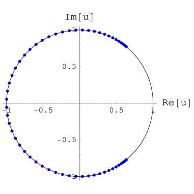
(a)

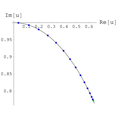
(b)

Figure 2: (Color online) Yang-Lee zeros for $N=60$ spins at $d\approx 0.8680$ and $c=0.48$. In figure (a) we have all zeros while figure (b) displays only the zeros on the first quadrant with the corresponding Yang-Lee edge singularity (green (light gray) dot). The solid line stands for $|u|=1$

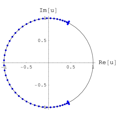
(a)

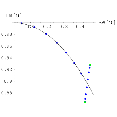
(b)

Figure 4: (Color online) Yang-Lee zeros and half of the Yang-Lee edge singularities (green (light gray) dots) for $N=60$ spins at $d\approx 0.8680$ and $c=0.52$

(a) Straight line: $\ln{\rm Re}(\Delta u)=2.022-2.996\,\ln N$ with $\chi^{2}_{E}=9.30\times 10^{-9}$

(b) Straight line: $\ln\rho=-5.341+1.987\,\ln N$ with $\chi^{2}_{\rho}=9.03\times 10^{-8}$

Figure 5: Log-log fits of (19) and (35) at $d\approx 0.8680$ and $c=0.5$ with $160\leq N\leq 240$ spins

$N_{a}$	$y_{h}^{\rho}$	$y_{h}^{E,\,Re}$	$y_{h}^{E,\,Im}$
160	2.984155688412	2.995280492398	2.995273778849
170	2.985057758429	2.995549136960	2.995543509484
180	2.985862192536	2.995788825553	2.995784061898
190	2.986584090647	2.996004003019	2.995999935011
200	2.987235580790	2.996198248276	2.996194746764
210	2.987826518204	2.996374475494	2.996371439968
220	2.988364995418	2.996535081652	2.996532432944
230	2.988857720521	2.996682056444	2.996679731514
$\infty$	3.00000000000(1)	3.00000000000(1)	3.00000000000(3)

Table 1: Finite size results for the Yang-Lee zeros, where $y_{h}^{\rho}$ are obtained from (36) while $y_{h}^{E,\,Re}$ and $y_{h}^{E,\,Im}$ come from (34) using the real and imaginary parts of the zeros respectively. The data of this table have been obtained from rings with $160\leq N\leq 240$ spins at $c=0.5$ and $d\approx 0.8680$. The last row is the $N\to\infty$ extrapolation via BST algorithm with $\omega=1$.

(a)

(b)

Figure 6: BST extrapolation for $0.1\leq\omega\leq 3.0$ of $y_{h}^{E}$ using the real part of the zeros (figure 6(a)) and $y_{h}^{\rho}$ (figure 6(b)) at $d\approx 0.8680$ and $c=0.5$.

References

• [1] C.N. Yang and T.D. Lee, Phys. Rev. 87 (1952) 404;
• [2] T.D. Lee and C.N. Yang, Phys. Rev. 87 (1952) 410.
• [3] R. B Griffiths, J. of Math. Phys. 10 (1969) 1559.
• [4] M. Suzuki, J. of Math. Phys. 14 (1973) 1088.
• [5] I. Bena, M. Droz; A. Lipowski, International J. Modern Phys. B 19(2005) 4269.
• [6] P. J. Kortman and R.B. Griffiths, Phys. Rev. Lett. 27 (1971) 1439.
• [7] Fisher M., Phys. Rev. Lett. 40 (1978) 1610.
• [8] J.L. Cardy, Phys. Rev. Lett. 54 1354 (1985).
• [9] V. Matveev and R. Schrock, Phys. Lett. A 215, 271 (1996).
• [10] S.-Y. Kim, Phys. Rev. E 74, 011119 (2006).
• [11] C. Binek in “Ising-type Antiferromagnets”, Springer-Verlag, Berlin (2003), C. Binek, Phys. Rev. Lett. 81 5644 (1998);
• [12] M. Fisher, Suppl. of the Progr. of Theor. Phys. 69(1980) 14.
• [13] D.A. Kurze, J. Stat. Phys. 30 15 (1983).
• [14] Z. Glumac and K. Uzelac, J. Phys. A 27 7709 (1994).
• [15] X.-Z. Wang and J. S. Kim, Phys. Rev. E 58, 4174 (1998).
• [16] R.G. Ghulghazaryan, K.G. Sargsyan, and N.S. Ananikian, Phys. Rev. E 76, 021104 (2007).
• [17] V.V. Hovhannisyana, R.G. Ghulghazaryana and N.S. Ananikian, Physica A 388 (2009) 1479.
• [18] L. Mittag and M.J. Stephen, J. Stat. Phys. 35 (1984) 303
• [19] D. Dalmazi and F.L. Sá, Phys. Rev. E 78(2008) 031138.
• [20] D. Dalmazi and F.L. Sá, J. Phys. A:Math Theor. 41(2008) 505002.
• [21] M. Blume, Phys. Rev. 141 (1966) 517; H.W. Capel, Physica 32 (1966) 966.
• [22] M. Blume, V.J. Emery, and R.B. Griffiths, Phys. Rev. A 4 1071 (1971).
• [23] R.J. Elliott, Phys. Rev. 124 (1961) 346.
• [24] M.E. Fisher and W. Selke. Phys. Rev. Lett. 44 (1980) 1502.
• [25] W. Selke, Physics Reports 170 No. 4 (1988) 213 264.
• [26] T. S. Nielsen and P.C. Hemmer, J. Chem. Phys. 46 2640 (1967).
• [27] C.Itzykson, R.B.Pearson and J.B.Zuber, Nucl. Phys. B 220(1983) 415.
• [28] E.N. Lassettre and J.P. Howe, J.Chem. Phys. 9(1941) 747.
• [29] J. Ashkin and W.E. Lamb, Phys. Rev 64(1943) 159.
• [30] R.J. Creswick and S.-Y. Kim, Phys. Rev. E 56(1997) 2418.
• [31] R. Bulirsch and J. Stoer, Numer. Math. 6 (1964) 413.
• [32] M. Henkel and G Schutz, J. Phys. A 21 (1988) 2617.
Refer to caption