Aspect-ratio dependence of thermodynamic Casimir forces

Abstract

We consider the three-dimensional Ising model in a $L_{\perp}\times L_{\parallel}\times L_{\parallel}$ cuboid geometry with finite aspect ratio $\rho=L_{\perp}/L_{\parallel}$ and periodic boundary conditions along all directions. For this model the finite-size scaling functions of the excess free energy and thermodynamic Casimir force are evaluated numerically by means of Monte Carlo simulations. The Monte Carlo results compare well with recent field theoretical results for the Ising universality class at temperatures above and slightly below the bulk critical temperature $T_{\mathrm{c}}$. Furthermore, the excess free energy and Casimir force scaling functions of the two-dimensional Ising model are calculated exactly for arbitrary $\rho$ and compared to the three-dimensional case. We give a general argument that the Casimir force vanishes at the critical point for $\rho=1$ and becomes repulsive in periodic systems for $\rho>1$.

I Introduction

The spatial confinement of a fluctuating and highly correlated medium may cause long-range forces. The Casimir effect, which was theoretically predicted in 1948 by the Dutch physicist H. B. G. Casimir Casimir (1948), is a prominent example. This quantum effect is caused by the vacuum fluctuations of the electromagnetic field and has been proven experimentally in the late 1990’s Lamoreaux (1997); Mohideen and Roy (1998). It becomes manifest in an attractive long-range Casimir force acting between two parallel, perfectly conducting plates in an electromagnetic vacuum.

Another example for a fluctuation-induced force being of similar nature as the Casimir force in quantum electrodynamics can be found in the physics of critical phenomena Fisher and de Gennes (1978); Gambassi (2009). This thermodynamic Casimir effect is caused by the spatial confinement of thermal fluctuations near the critical point of a second order phase transition. Experimentally, it has been proven for the first time by measuring the film thickness of superfluid ⁴He films as a function of the temperature in the vicinity of the lambda transition Garcia and Chan (1999); Ganshin et al. (2006). Since then, the thermodynamic Casimir effect was measured in several different systems including binary liquid mixtures Fukuto et al. (2005); Hertlein et al. (2008); Gambassi et al. (2009) and tricritical ³He-⁴He Garcia and Chan (2002).

For several years the shape of the finite-size scaling function determined by Garcia and Chan Garcia and Chan (1999) from the experimental data has not been understood theoretically, in particular its deep minimum right below $T_{\mathrm{c}}$. While the value of the Casimir force at criticality as well as the decay above $T_{\mathrm{c}}$ could be calculated using field theory Krech and Dietrich (1992); Krech (1994); Diehl et al. (2006); Grüneberg and Diehl (2008), no quantitative results were available for the scaling region $T\lesssim T_{\mathrm{c}}$ except for mean-field-theoretical approaches Maciołek et al. (2007); Zandi et al. (2007). Analytic results exist only for the non-critical region below $T_{\mathrm{c}}$, where contributions to the thermodynamic Casimir force from Goldstone modes Li and Kardar (1991, 1992); Kardar and Golestanian (1999) and from the excitation of capillary waves of the liquid-vapor ⁴He interface Zandi et al. (2004) become dominant.

This unsatisfactory situation was resolved in Ref. Hucht (2007), where a method was proposed to calculate the thermodynamic Casimir force for $O(n)$-symmetrical lattice models using Monte Carlo simulations without any approximations, in contrast to, e. g., the stress tensor method used by Dantchev and Krech Dantchev and Krech (2004), which furthermore was restricted to periodic systems. The Monte Carlo simulations were done for the three-dimensional (3D) XY model on a simple cubic lattice with film geometry $L_{\perp}\times L_{\parallel}\times L_{\parallel}$ and open boundary conditions along the $\perp$-direction, as this system is known to be in the same universality class as the superfluid transition in ⁴He and thus displays the same asymptotic critical behavior. The results were found to be in excellent agreement with the experimental results by Garcia, Chan and coworkers Garcia and Chan (1999); Ganshin et al. (2006) and for the first time provided a theoretical explanation for the characteristic shape of the finite-size scaling function and in particular its deep minimum below $T_{\mathrm{c}}$. In the following, this method was used to determine Casimir forces in various systems and geometries Hasenbusch (2010, 2010), while other methods for the evaluation of thermodynamic Casimir forces using Monte Carlo simulations have also been presented Vasilyev et al. (2007); Hasenbusch (2009, 2009).

In the present work, this method is used to derive the universal finite-size scaling function of the excess free energy and thermodynamic Casimir force as functions of the aspect ratio $\rho=L_{\perp}/L_{\parallel}$ for the 3D Ising model with cuboid geometry and periodic boundary conditions. Here $\rho$ is allowed to take arbitrary values from $\rho\to 0$ (film geometry) to $\rho\to\infty$ (rod geometry), while former investigations were either at $\rho=0$ Krech and Dietrich (1992); Krech (1994); Diehl et al. (2006); Grüneberg and Diehl (2008); Maciołek et al. (2007); Zandi et al. (2007) or limited to the case $\rho\ll 1$ Dantchev and Krech (2004); Hucht (2007); Vasilyev et al. (2007); Hasenbusch (2009, 2010, 2009); Vasilyev et al. (2009); Hasenbusch (2010); Toldin and Dietrich (2010). The paper is structured as follows: In the remainder of Sec. I the basic principles and definitions concerning the thermodynamic Casimir effect are discussed and the Monte Carlo method will be revisited. In Sec. II, our Monte Carlo results are discussed and compared to recently published results by Dohm Dohm (2009) who calculated the Casimir force within a minimal renormalization scheme of the $O(n)$ model at finite $\rho$, covering temperatures below and above $T_{\mathrm{c}}$, as well as to field-theoretical results obtained for $T\geq T_{\mathrm{c}}$ in the framework of the renormalization group-improved perturbation theory (RG) to two-loop order Diehl et al. (2006); Grüneberg and Diehl (2008). In Sec. III, we present an exact calculation of the excess free energy and Casimir force scaling functions for the two-dimensional (2D) Ising model with arbitrary aspect ratios $\rho$. We conclude with a discussion and a summary.

I.1 Basic principles

When a thermodynamical system in $d$ dimensions such as a simple classical fluid or a classical $n$-vector magnet is confined to a region with thickness $L_{\perp}$ and cross-sectional area $L_{\parallel}^{d-1}$, its total free energy $F$ becomes explicitly size-dependent. Then the reduced free energy per unit volume

$$f(T,L_{\perp},L_{\parallel}) \equiv \frac{F(T,L_{\perp},L_{\parallel})}{L_{\perp}L_{\parallel}^{d-1}k_{\text{B}}T}$$ (1)

$$= f_{\infty}(T)+\delta f(T,L_{\perp},L_{\parallel})$$

can be decomposed Privman (1990) into a sum of the bulk free energy density $f_{\infty}$ and a finite-size contribution $\delta f$. As we assume periodic boundary conditions in all directions, the surface terms in $\perp$ and $\parallel$ directions as well as edge and corner contributions are omitted in (1). In this case the residual free energy $\delta f$ equals the excess free energy $f_{\mathrm{ex}}$, and we will use $f_{\mathrm{ex}}$ instead of $\delta f$ in the following.

In terms of $f_{\mathrm{ex}}$ the reduced thermodynamic Casimir force per surface area in $\perp$ direction is defined as Krech (1994)

$$\beta\mathcal{F}_{\mathrm{C}}(T,L_{\perp},L_{\parallel})\equiv-\frac{\partial[L_{\perp}f_{\mathrm{ex}}(T,L_{\perp},L_{\parallel})]}{\partial L_{\perp}},$$ (2)

where $\beta=1/k_{\text{B}}T$, and the derivative is taken at fixed $L_{\parallel}$. We omit the index $\perp$ for the Casimir force, as we will not consider Casimir forces in parallel directions in this work.

When in the absence of symmetry breaking external fields the critical point is approached from higher temperatures, which corresponds to the liquid-vapor critical point in the case of a simple classical fluid or to the Curie point in a classical $n$-vector magnet, the bulk correlation length $\xi_{\infty}(t)$ grows and diverges as

$$\xi_{\infty}(t)\underset{t>0}{\sim}\xi_{+}t^{-\nu},$$ (3)

with correlation length exponent $\nu$, reduced temperature $t=T/T_{\text{c},\infty}-1$, and non-universal amplitude $\xi_{+}$. In this work we use $\xi_{+}=Q_{\xi}^{+}f^{+}=1.000183(2)\times 0.506(1)$ valid for the 3D Ising model on a simple cubic lattice Campostrini et al. (1999); Butera and Comi (2002).

According to the theory of finite-size scaling Fisher (1971) and under the assumption, that long-range interactions and other contributions irrelevant in the RG sense are negligible, as for instance subleading long-range interactions Dantchev et al. (2006), the thermodynamic Casimir force in the regime $L_{\perp},L_{\parallel},\xi_{\infty}\gg a$, where $a$ is a characteristic microscopic length scale such as the lattice constant in the case of a lattice model, obeys a finite-size scaling form

$$\beta\mathcal{F}_{\mathrm{C}}(T,L_{\perp},L_{\parallel})\sim L_{\perp}^{-d}\vartheta_{\perp}(x_{\perp},\rho),$$ (4)

where the scaling variable $x_{\perp}$ can be defined as

$$x_{\perp}\equiv t\left(\frac{L_{\perp}}{\xi_{+}}\right)^{\frac{1}{\nu}}\underset{t>0}{\sim}\left(\frac{L_{\perp}}{\xi_{\infty}(t)}\right)^{\frac{1}{\nu}},$$ (5)

$\rho=L_{\perp}/L_{\parallel}$ denotes the aspect ratio, and $\vartheta_{\perp}$ is a finite-size scaling function. Note that in this work $\vartheta$ always denotes the scaling function of the Casimir force in $\perp$ direction, while the index describes the reference direction $\perp$ or $\parallel$ of length $L$.

An analogous finite-size scaling relation holds for the excess free energy,

$$f_{\mathrm{ex}}(T,L_{\perp},L_{\parallel})\sim L_{\perp}^{-d}\Theta_{\perp}(x_{\perp},\rho),$$ (6)

and $\vartheta_{\perp}$ is related to $\Theta_{\perp}$ according to Dohm (2009)

$$\vartheta_{\perp}(x_{\perp},\rho)=\left[d-1-\frac{1}{\nu}\frac{x_{\perp}\partial}{\partial x_{\perp}}-\frac{\rho\partial}{\partial\rho}\right]\Theta_{\perp}(x_{\perp},\rho).$$ (7)

The dimensionless finite-size scaling functions $\Theta_{\perp}$ and $\vartheta_{\perp}$ are universal, that is, they only depend on gross properties of the system such as the bulk and surface universality classes of the phase transition, the system shape and boundary conditions, but not on its microscopic details Grüneberg and Hucht (2004); Dantchev et al. (2006).

At the critical point $T_{\mathrm{c}}$ the thermodynamic Casimir force becomes long-ranged and for sufficiently large values of the length $L_{\perp}$ asymptotically decays as

$$\beta\mathcal{F}_{\mathrm{C}}(T_{\mathrm{c}},L_{\perp},L_{\parallel}) \sim L_{\perp}^{-d}\vartheta_{\perp}(0,\rho)$$ (8)

$$\sim L_{\perp}^{-d}[(d-1)\Delta_{\perp}(\rho)-\rho\Delta_{\perp}^{\prime}(\rho)],$$

where $\Delta_{\perp}(\rho)\equiv\Theta_{\perp}(0,\rho)$ is the so-called Casimir amplitude Fisher and de Gennes (1978), being – like the finite-size scaling function $\vartheta_{\perp}$ – an universal quantity. Note that for finite aspect ratios $\rho>0$ the Casimir amplitude becomes $\rho$-dependent. The film geometry is recovered by letting $\rho\rightarrow 0$, and Eq. (8) simplifies to

$$\beta\mathcal{F}_{\mathrm{C}}(T_{\mathrm{c}},L_{\perp},\infty)\sim L_{\perp}^{-d}(d-1)\Delta_{\perp}(0).$$ (9)

Since the 1990s, such universal quantities have been subject of extensive theoretical research. They were studied by means of exactly solvable models Krech (1994); Danchev (1998); Brankov et al. (2000); Dantchev et al. (2003); Dantchev and Krech (2004); Dantchev et al. (2006); Dantchev and Grüneberg (2009), Monte Carlo simulations Krech and Landau (1996); Dantchev and Krech (2004); Hucht (2007); Vasilyev et al. (2007); Maciołek et al. (2007); Hertlein et al. (2008); Hasenbusch (2009, 2010, 2009); Vasilyev et al. (2009); Hasenbusch (2010), as well as within field-theoretical approaches Krech and Dietrich (1992); Krech (1994); Diehl et al. (2006); Grüneberg and Diehl (2008); Schmidt and Diehl (2008); Diehl and Grüneberg (2009); Dohm (2009); Burgsmüller et al. (2010).

I.2 Reformulation for arbitrary $\rho$

The formulation of the Casimir force finite-size scaling laws in the previous section was done by assuming film geometry $\rho\ll 1$, i. e., having in mind the limit $\rho\rightarrow 0$. However, if $\rho\gtrsim 1$ this picture is not appropriate and should be replaced by a more general treatment. In the following we rewrite the basic scaling laws in terms of the system volume $V=L_{\perp}L_{\parallel}^{d-1}$ instead of the film thickness $L_{\perp}$. The resulting scaling functions can be used in the whole regime $0<\rho<\infty$.

Using the substitution $L_{\perp}^{d}\to V\rho^{d-1}$ in Eq. (6) we get

$$f_{\mathrm{ex}}(T,L_{\perp},L_{\parallel})\sim V^{-1}\Theta(x,\rho)$$ (10)

with an universal scaling function $\Theta$ and the generalized scaling variable

$$x\equiv t\left(\frac{V}{\xi_{+}^{d}}\right)^{\frac{1}{d\nu}},$$ (11)

while the scaling function $\Theta_{\perp}$ from Eq. (6) is recovered as

$$\Theta_{\perp}(x_{\perp},\rho)=\rho^{d-1}\Theta(x,\rho),$$ (12)

with

$$x_{\perp}=\rho^{\frac{1}{\nu}-\frac{1}{d\nu}}x.$$ (13)

Similarly, the Casimir force obeys

$$\beta\mathcal{F}_{\mathrm{C}}(T,L_{\perp},L_{\parallel})\sim V^{-1}\vartheta(x,\rho),$$ (14)

from which we derive the scaling identity

$$\vartheta(x,\rho)=-\left[\frac{1}{d\nu}\frac{x\partial}{\partial x}+\frac{\rho\partial}{\partial\rho}\right]\Theta(x,\rho).$$ (15)

Note that this identity is equivalent to but simpler than Eq. (7). At criticality we now define the generalized Casimir amplitude as

$$\Delta(\rho)=\Theta(0,\rho)$$ (16)

and find

$$f_{\mathrm{ex}}(T_{\mathrm{c}},L_{\perp},L_{\parallel}) \sim V^{-1}\Delta(\rho),$$ (17)

$$\beta\mathcal{F}_{\mathrm{C}}(T_{\mathrm{c}},L_{\perp},L_{\parallel}) \sim -V^{-1}\rho\Delta^{\prime}(\rho).$$ (18)

The case $\rho=1$ deserves special attention: As

$$\left.\frac{\partial}{\partial\rho}\Theta(x,\rho)\right|_{\rho=1}=0$$ (19)

in cubic geometry (see Appendix A), Eq. (15) simplifies to

$$\vartheta(x,1)=-\frac{1}{d\nu}\frac{x\partial}{\partial x}\Theta(x,1)$$ (20)

at $\rho=1$, and gives a remarkably simple connection between the Casimir force and the excess internal energy, Eq. (30), in the cube shaped system, namely

$$\beta\mathcal{F}_{\mathrm{C}}(T,L,L)\sim\frac{t}{d\nu}\,u_{\mathrm{ex}}(T,L,L).$$ (21)

Obviously, the Casimir force vanishes at the critical point if $\rho=1$, i. e.,

$$\vartheta(0,1)=0.$$ (22)

For completeness we also give the definitions of the scaling functions in terms of $L_{\parallel}$. As

$$f_{\mathrm{ex}}(T,L_{\perp},L_{\parallel})\sim L_{\parallel}^{-d}\Theta_{\parallel}(x_{\parallel},\rho),$$ (23)

we find

$$\Theta_{\parallel}(x_{\parallel},\rho)=\rho^{-1}\Theta(x,\rho)$$ (24)

with $x_{\parallel}\equiv t(L_{\parallel}/\xi_{+})^{1/\nu}$. Note that in this representation the scaling identity Eq. (7) reads

$$\vartheta_{\parallel}(x_{\parallel},\rho)=-\left[1+\frac{\rho\partial}{\partial\rho}\right]\Theta_{\parallel}(x_{\parallel},\rho)$$ (25)

and in the limit $\rho\to\infty$ simplifies to

$$\vartheta_{\parallel}(x_{\parallel},\infty)=-\Theta_{\parallel}(x_{\parallel},\infty),$$ (26)

leading to the simple relation

$$\beta\mathcal{F}_{\mathrm{C}}(T,\infty,L_{\parallel})\sim-f_{\mathrm{ex}}(T,\infty,L_{\parallel}).$$ (27)

I.3 Monte Carlo method

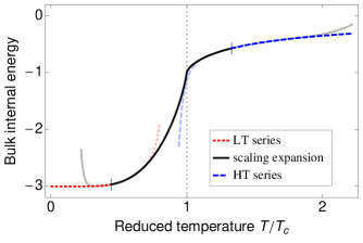
Figure 1: (Color online) Bulk internal energy density $e_{\infty}(T)$ obtained from three different methods: low temperature series Bhanot et al. (1994) (red dotted line), scaling expansion Feng and Blöte (2010) (black line), and high temperature series Arisue and Fujiwara (2003) (blue dashed line).

In this work we focus on the three-dimensional isotropic nearest neighbor Ising model on a $L_{\perp}\times L_{\parallel}\times L_{\parallel}$ simple cubic lattice with periodic boundary conditions and Hamiltonian

$$\beta\mathcal{H}=-\frac{K}{2}\sum_{\langle ij\rangle}\sigma_{i}\sigma_{j},$$ (28)

where $K=\beta J>0$ is the ferromagnetic reduced exchange interaction and $\sigma_{i}=\pm 1$ are one-component spin variables at lattice sites $i$. The Monte Carlo simulations were done using the Wolff single cluster algorithm Wolff (1989). Measuring the reduced internal energy density

$$u(T,L_{\perp},L_{\parallel})=\frac{\langle\beta\mathcal{H}\rangle}{L_{\parallel}^{d-1}L_{\perp}},$$ (29)

the excess free energy and Casimir force is calculated as follows Hucht (2007): First we determined the excess internal energy

$$u_{\text{ex}}(T,L_{\perp},L_{\parallel})\equiv u(T,L_{\perp},L_{\parallel})-u_{\infty}(T)$$ (30)

by subtracting the reduced bulk internal energy density $u_{\infty}(T)$. We used three different results to get precise estimates for $u_{\infty}(T)$ of the $3d$ Ising model in the different temperature regimes: For low temperatures $K>1/2$ we used the low temperature series expansion (54th order) by Bhanot et al. Bhanot et al. (1994), while for $K<1/6$ the high temperature series expansion (46th order) by Arisue and Fujiwara Arisue and Fujiwara (2003) was utilized. Finally, in the vicinity of the critical point we used the expansion recently obtained by Feng and Blöte Feng and Blöte (2010), where we also took the bulk critical indices Deng and Blöte (2003) $K_{\mathrm{c}}=0.22165455(3)$, $\nu^{-1}=1.5868(3)$ and $\omega=0.821(5)$. These three estimates of $u_{\infty}(T)$ show a broad overlap, see also the discussion by Feng and Blöte Feng and Blöte (2010), the resulting non-reduced bulk internal energy density $e_{\infty}(T)=u_{\infty}(T)/\beta$ is depicted in Fig. 1. With the identity

$$f_{\mathrm{ex}}(T,L_{\perp},L_{\parallel})=-\int_{T}^{\infty}\frac{\mathrm{d}\tau}{\tau}u_{\mathrm{ex}}(\tau,L_{\perp},L_{\parallel})$$ (31)

we determined $f_{\mathrm{ex}}$ by numerical integration, using the fact that $u_{\mathrm{ex}}$ goes exponentially fast to zero above $T_{\mathrm{c}}$ Hucht (2007).

To obtain the Casimir force, we first calculated the internal Casimir force

$$\beta\mathcal{F}_{\mathrm{I}}(T,L_{\perp},L_{\parallel})=-\frac{\partial[L_{\perp}u_{\text{ex}}(T,L_{\perp},L_{\parallel})]}{\partial L_{\perp}},$$ (32)

which is defined similar to Eq. (2), by numerical differentiation, using thicknesses $L_{\perp}^{\prime}=L_{\perp}\pm 1$ in order to get an integral effective thickness $L_{\perp}$. With Eqs. (4, 35) and the hyperscaling relation $d\nu=2-\alpha$ with specific heat exponent $\alpha$, it is straightforward to show that this quantity fulfills the finite-size scaling form

$$-\beta\mathcal{F}_{\mathrm{I}}(T,L_{\perp},L_{\parallel})\sim\xi_{+}^{-1/\nu}L_{\perp}^{(\alpha-1)/\nu}\vartheta_{\perp}^{\prime}(x_{\perp},\rho),$$ (33)

with an universal finite-size scaling function

$$\vartheta_{\perp}^{\prime}(x_{\perp},\rho)=\frac{\partial\vartheta_{\perp}(x_{\perp},\rho)}{\partial x_{\perp}}.$$ (34)

This quantity turns out to be very useful in understanding the Casimir force scaling function $\vartheta_{\perp}(x_{\perp},\rho)$ for $\rho\to 0$, as will be shown in the next section. Finally, the thermodynamic Casimir force is obtained from Eq. (32) by integration,

$$\beta\mathcal{F}_{\mathrm{C}}(T,L_{\perp},L_{\parallel})=-\int_{T}^{\infty}\frac{\mathrm{d}\tau}{\tau}\beta\mathcal{F}_{\mathrm{I}}(\tau,L_{\perp},L_{\parallel}),$$ (35)

where again the exponential decay above $T_{\mathrm{c}}$ simplifies the numerical integration.

II Results

II.1 Casimir force in film geometry $\rho\to 0$

In Fig. 2 we plot the internal Casimir force $\beta\mathcal{F}_{\mathrm{I}}$, Eq. (32), for small aspect ratios $\rho=1/8$ and $\rho=1/16$. In the limit of film geometry $\rho\to 0$ we observe strong finite-size effects below the critical point Hucht (2007), which are caused by the influence of the phase transition in the $d{-}1$-dimensional system. In this section we will analyse this influence in detail and show that $\beta\mathcal{F}_{\mathrm{I}}$ is directly connected to the specific heat of the $d{-}1$-dimensional system. We will give the derivation for periodic systems where no surface terms occur, as these terms will complicate the analysis Hasenbusch (2010).

From the scaling identity Eq. (7) for $\rho\to 0$,

$$\vartheta_{\perp}(x_{\perp},0)=\left[d-1-\frac{1}{\nu}\frac{x_{\perp}\partial}{\partial x_{\perp}}\right]\Theta_{\perp}(x_{\perp},0)$$ (36)

we get

$$\beta\mathcal{F}_{\mathrm{C}}\underset{\rho\to 0}{\sim}(d-1)f_{\mathrm{ex}}+t\,\nu^{-1}\,u_{\mathrm{ex}},$$ (37)

i. e., within the scaling region and for $\rho\text{$\to$0 }$ the Casimir force can alternatively be calculated without $L_{\perp}$-derivative Hasenbusch (2010). For the internal Casimir force scaling function

$$\vartheta_{\perp}^{\prime}(x_{\perp},0)=\left[d-1-\frac{1}{\nu}-\frac{1}{\nu}\frac{x_{\perp}\partial}{\partial x_{\perp}}\right]\frac{\partial\Theta_{\perp}(x_{\perp},0)}{\partial x_{\perp}}$$ (38)

we find the asymptotic identity

$$-\beta\mathcal{F}_{\mathrm{I}}\underset{\rho\to 0}{\sim}-\left[d-1-\frac{1-t}{\nu}\right]\,u_{\mathrm{ex}}+\frac{t}{\nu}\,c_{\mathrm{ex}}$$ (39)

with the excess specific heat

$$c_{\mathrm{ex}}(T,L_{\perp},L_{\parallel})\equiv c(T,L_{\perp},L_{\parallel})-c_{\infty}(T)$$ (40)

and $c=\partial Tu/\partial T$ as usual. For $\rho\to 0$, this quantity contains both the bulk singularity

$$c_{\infty}(T)\sim A_{\pm}\left|t\right|^{-\alpha},$$ (41)

with amplitudes $A_{\pm}$, as well as the singularity of the laterally infinite film with finite thickness $L_{\perp}$ at $t_{\mathrm{c}}(L_{\perp})=T_{\mathrm{c}}(L_{\perp})/T_{\mathrm{c}}-1$, which scales as

$$c(T,L_{\perp},\infty)\sim A_{\pm}^{*}\left(\frac{L_{\perp}}{\xi_{+}}\right)^{\frac{\alpha-\alpha^{*}}{\nu}}\left|t-t_{\mathrm{c}}(L_{\perp})\right|^{-\alpha^{*}}.$$ (42)

Here, $\alpha^{*}$ denotes the specific heat exponent of the $d{-}1$-dimensional system, $A_{\pm}^{*}$ are amplitudes, and the factor $(L_{\perp}/\xi_{+})^{(\alpha-\alpha^{*})/\nu}$ guarantees the correct scaling behavior for $L_{\perp}\to\infty$ by cancellation of terms containing $\alpha^{*}$.

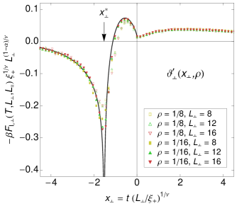
Figure 2: (Color online) Internal Casimir force scaling function $\vartheta_{\perp}^{\prime}(x_{\perp},\rho)$ for small aspect ratios $\rho=1/16$ and $\rho=1/8$. The black thin line is the extrapolation $\rho\to 0$, showing a logarithmic singularity at $x_{\perp}^{*}=1.535(10)$ (see text).

However, as $c_{\mathrm{ex}}$ enters Eq. (39) with prefactor $t$ only, the bulk singularity at $t=0$ is suppressed (as $\alpha<1$) and $c_{\mathrm{ex}}$ is dominated by the singularity from Eq. (42), at

$$x_{\perp}^{*}\sim t_{\mathrm{c}}(L_{\perp})\,\left(\frac{L_{\perp}}{\xi_{+}}\right)^{\frac{1}{\nu}}.$$ (43)

The location of the critical point was re-analysed from the data of Kitatani et al. Kitatani et al. (1996) including corrections to scaling, as well as from the data of Caselle and Hasenbusch Caselle and Hasenbusch (1996), giving the value $x_{\perp}^{*}=-1.535(10)$. This improves the value $x_{\perp}^{*}=-1.60(2)$ found by Vasilyev et al. Vasilyev et al. (2009). Furthermore, the other terms in (39) are $O(1)$ near $x_{\perp}^{*}$, which leads us to the conclusion that the specific heat singularity of the $d{-}1$-dimensional film is directly visible in the scaling function $\vartheta_{\perp}^{\prime}(x_{\perp},0)$ around $x_{\perp}=x_{\perp}^{*}$,

$$\vartheta_{\perp}^{\prime}(x_{\perp}\approx x_{\perp}^{*},0)\sim\frac{A_{\pm}^{*}\xi_{+}^{d}}{\nu}\,x_{\perp}|x_{\perp}-x_{\perp}^{*}|^{-\alpha^{*}}+\mathcal{O}(1).$$ (44)

From this arguments we conclude that the scaling function $\vartheta_{\perp}^{\prime}(x_{\perp},0)$ has a singularity at $x_{\perp}^{*}$ dominated by the specific heat singularity of the $d{-}1$-dimensional system, with critical exponent $\alpha^{*}$. In our case, $\alpha^{*}=0$ and the singularity is logarithmic. This asymptotic behavior is included in Fig. 2 as solid line.

In Fig. 3 we show the scaling function of the Casimir force for $\rho=1/8,1/16$, together with the RG results of Grüneberg and Diehl Grüneberg and Diehl (2008). The solid line is the integrated extrapolation discussed above. We used a correction factor $(1+g_{1}L_{\perp}^{-2})$, with $g_{1}=-4(1)$, to account for leading systematic errors from the discrete derivative, which are expected to be $\propto L_{\perp}^{-2}$ in periodic systems. The inset is a magnification of the minimum, from the divergence of $\vartheta_{\perp}^{\prime}(x_{\perp}{=}x_{\perp}^{*},0)$ the slope of $\vartheta_{\perp}(x_{\perp},0)$ at $x_{\perp}^{*}$ diverges logarithmically. We find a critical amplitude $\vartheta_{\perp}(0,0)=-0.310(6)$ (see Tab. 1), which agrees within error bars with the values $\vartheta_{\perp}(0,0)=-0.3040(4)$ Vasilyev et al. (2009) as well as $\vartheta_{\perp}(0,0)=-0.3052(20)$ Krech (1997). The zero at $\vartheta_{\perp}^{\prime}(x_{\perp}^{\mathrm{min}},0)$ (solid line in Fig. 2) gives the minimum position $x_{\perp}^{\mathrm{min}}=-1.13(5)$, with $\vartheta_{\perp}(x_{\perp}^{\mathrm{min}},0)=-0.360(5)$, while the finite $\rho$ results are $\vartheta_{\perp}(x_{\perp}^{\mathrm{min}}=-1.10(5),1/16)=-0.352(5)$ and $\vartheta_{\perp}(x_{\perp}^{\mathrm{min}}=-0.95(5),1/8)=-0.340(5)$.

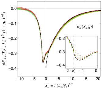
Figure 3: (Color online) Casimir force scaling function $\vartheta_{\perp}(x_{\perp},\rho)$ for small aspect ratios $\rho=1/16$ and $\rho=1/8$. The solid line is the extrapolation $\rho\to 0$ calculated from the integrated logarithmic singularity in $\vartheta_{\perp}^{\prime}(x_{\perp},0)$. The dotted line is the RG calculation of Grüneberg and Diehl Grüneberg and Diehl (2008).

II.2 Casimir force for finite $\rho$

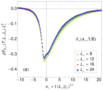
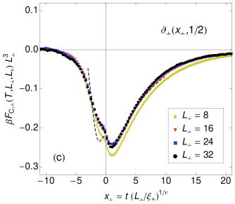
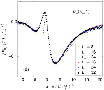
Figure 4: (Color online) Casimir force scaling function $\vartheta_{\perp}(x_{\perp},\rho)$ for several aspect ratios $\rho=\{1/6,1/4,1/2,1\}$. The dotted line is the result of Grüneberg and Diehl Grüneberg and Diehl (2008) for $\rho=0$, while the dashed lines are the predictions of Dohm Dohm (2009). For $\rho=1$ we also show results from scaling relation Eq. (20) (filled symbols), which have much better statistics, as they are directly calculated from the internal energy.

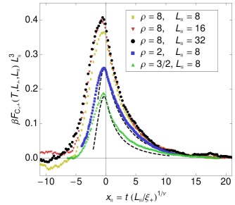
Figure 5: (Color online) Casimir force scaling function $\vartheta_{\parallel}(x_{\parallel},\rho)$ for aspect ratios $\rho>1$, now as function of the proper scaling variable $x_{\parallel}$. The dashed lines are the predictions of Dohm Dohm (2009).

If we increase $\rho$ to finite values, the Casimir force scaling function $\vartheta_{\perp}(x_{\perp},\rho)$ first changes its shape around the minimum. The results for $\rho=1/6$ (Fig. 4a) already deviate distinctly from the thinner systems, the minimum below $T_{\mathrm{c}}$ is not so deep anymore, with $\vartheta_{\perp}(x_{\perp}^{\mathrm{min}}=-0.77(5),1/6)=-0.323(5)$. These values deviate only slightly from the results of Vasilyev et al. Vasilyev et al. (2009), $x_{\perp}^{\mathrm{min}}=-0.681(1)$ and $\vartheta_{\perp}(x_{\perp}^{\mathrm{min}},1/6)=-0.329(1)$, which we attribute to the larger statistical error in Ref. Vasilyev et al. (2009).

When the aspect ratio is further increased to $\rho=1/4$ (Fig. 4b), the curve has two minima below and above $T_{\mathrm{c}}$ which are nearly equal in depth. Note that the results for $\rho\geq 1/4$ are compared to the predictions of Dohm Dohm (2009) and show similar behavior. For $\rho\gtrsim 1/4$ the minimum below $T_{\mathrm{c}}$ vanishes, while the one above $T_{\mathrm{c}}$ remains. This is shown in Fig. 4c, where we plot the Casimir scaling function for $\rho=1/2$.

The results for the cube shaped system with $\rho=1$ are shown in Fig. 4d . The case $\rho=1$ is quite interesting, as here the Casimir force at $x=0$ vanishes (Eq. (22)) and even becomes positive for $\rho>1$, although the system has symmetric, i. e., periodic boundary conditions. However, this sign change of the Casimir force at $\rho=1$ does not contradict the predictions of Bachas Bachas (2007), as he assumed an infinite system in parallel direction, i. e., $\rho=0$. The scaling function $\vartheta(x,1)$ has negative slope $\vartheta^{\prime}(0,1)=-\Theta^{\prime}(0,1)/d\nu$ at $x=0$. This behavior is in perfect agreement with Eq. (21), as the excess internal energy $u_{\mathrm{ex}}(T_{\mathrm{c}},L,L)$ is negative for our model. Furthermore, $\vartheta(x,1)$ has a second zero at $x=-2.25(5)$ where $u(T,L,L)=u_{\infty}(T)$ holds. Fig. 4d shows results from both the calculation using Eqs. (29-35) (open symbols) as well as Eq. (21) (filled symbols), where the latter have a much better statistics, as no numerical differentiation and integration is necessary.

Finally, in Fig. 5 we depict the Casimir scaling function for values of $\rho$ larger than one. Now we are in rod geometry and use the appropriate scaling variable $L_{\parallel}$ instead of $L_{\perp}$. Due to this rescaling, the scaling function $\vartheta_{\parallel}(x_{\parallel},\rho)$ converges to a finite limit $\vartheta_{\parallel}(x_{\parallel},\infty)$ which should only slightly deviate from curves for $\rho=8$, just as in the inverse case $\rho=1/8$ (see Fig. 3). In this regime the Casimir force is always positive, leading to a repulsion of the opposite surfaces. Note that for $\rho=8$ we increased the thickness difference for the calculation of the derivative in Eq. (32) to $L_{\perp}^{\prime}=L_{\perp}\pm 4$, as, e. g., $L_{\perp}=256$ for $L_{\parallel}=32$.

II.3 Excess free energy

The excess free energy is shown in Fig. 6 for $\rho\leq 1$. An interesting feature of these curves is the non-vanishing limit for $x_{\perp}\to-\infty$, which means that for fixed temperatures $T<T_{\mathrm{c}}$ and $L_{\perp},L_{\parallel}\to\infty$ the total excess free energy $Vf_{\mathrm{ex}}$ approaches a finite value. This behavior is a direct consequence of the broken symmetry in the ordered phase Privman and Fisher (1983): In this phase, which only exists in the thermodynamic limit below $T_{\mathrm{c}}$, the Ising partition function is reduced by a factor of two, as the system cannot reach the whole phase space anymore. This leads to the term $-\ln 2$ in the total excess free energy of a periodic Ising system below $T_{\mathrm{c}}$,

$$\Theta(-\infty,\rho)=-\ln 2,$$ (45)

independent of shape and dimensionality. Note that, e. g., for the $q$-state Potts model this argument directly generalizes to $\Theta(-\infty,\rho)=-\ln q$. Using Eq. (12), we find

$$\Theta_{\perp}(-\infty,\rho)=-\rho^{d-1}\ln 2,$$ (46)

this limit is shown as thin solid lines in Fig. 6. The results are compared to the field theoretical predictions of Dohm Dohm (2009), we find a satisfactory agreement for positive and also for slightly negative values of $x_{\perp}$. Furthermore, our value $\Delta(1)=-0.63(1)$ for the cube is compatible with the value $-0.657(30)$ obtained by Mon Mon (1985).

Figure 6: (Color online) Excess free energy scaling function $\Theta_{\perp}(x_{\perp},\rho)$ for several aspect ratios $\rho$. The dashed lines are the predictions of Dohm Dohm (2009) for $\rho=1/4,1/2,1$, while the solid lines are the limits for $x_{\perp}\to-\infty$, Eq. (46).

The generalized Casimir amplitude at criticality, $\Delta(\rho)=\Theta(0,\rho)$ (Eq. (16)), is listed in Tab. 1 for several values of $\rho$ and is depicted in Fig. 7, together with the predictions of Dohm Dohm (2009) (dashed line) as well as the asymptotes (dotted lines). The inset shows $\Delta_{\perp}(\rho)$ (circles) and $\Delta_{\parallel}(1/\rho)$ (squares), showing good agreement with these predictions for $1/4\lesssim\rho\lesssim 3$.

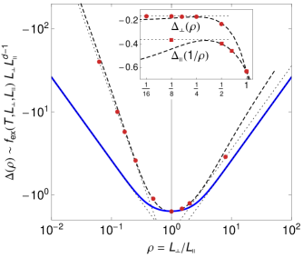
Figure 7: (Color online) Generalized Casimir amplitude $\Delta(\rho)=\Theta(0,\rho)$, Eq. (16), of the Ising universality class in $d=3$ (red circles, see also Tab. 1) and in $d=2$ (Eq. (56), blue solid line). The dashed line is the prediction of Dohm Dohm (2009), while the dotted lines show the asymptotes. The inset depicts $\Delta_{\perp}(\rho)$ (circles) and $\Delta_{\parallel}(1/\rho)$ (squares).

Table 1: Monte Carlo results for the Casimir amplitudes $\Delta(\rho)$, $\Delta_{\mu}(\rho)$ and $\vartheta_{\mu}(0,\rho)$, with $\mu=\perp$ for $\rho\leq 1$ and $\mu=\parallel$ for $\rho\geq 1$. Note that the critical Casimir force changes sign at $\rho=1$.

$\rho$	$\Delta(\rho)$	$\Delta_{\mu}(\rho)$	$\vartheta_{\mu}(0,\rho)$
$0$	$-\infty$	$-0.155(3)$	$-0.310(6)$
$1/16$	$-39.8(8)$	$-0.155(3)$	$-0.310(6)$
$1/8$	$-9.9(2)$	$-0.155(3)$	$-0.310(6)$
$1/6$	$-5.7(1)$	$-0.157(3)$	$-0.30(1)$
$1/4$	$-2.60(5)$	$-0.161(3)$	$-0.290(5)$
$1/2$	$-0.89(2)$	$-0.223(4)$	$-0.22(1)$
$1$	$-0.63(1)$	$-0.63(1)$	$0.000(5)$
$3/2$	$-0.68(3)$	$-0.45(2)$	$0.17(1)$
$2$	$-0.78(3)$	$-0.39(2)$	$0.25(1)$
$8$	$-2.86(5)$	$-0.357(8)$	$0.36(1)$
$\infty$	$-\infty$	$-0.36(1)$	$0.36(1)$

III Exact results in two dimensions

The scaling function $\Theta_{\perp}$ of the excess free energy in $d=2$ is calculated exactly based on the work of Ferdinand and Fisher Ferdinand and Fisher (1969) (Note that the term $\xi S_{1}(n)\tau^{2}/2$ is missing in Eq. (3.36) of this work). Our scaling variables differ from theirs, we use $x_{\perp}=t(L_{\perp}/\xi_{+})$ and $\rho=L_{\perp}/L_{\parallel}$, while they used $\tau=x_{\perp}/2$ and $\xi=1/\rho$ as temperature and aspect-ratio variables.

We start from the partition function of the $L_{\perp}\times L_{\parallel}$ isotropic Ising model on a torus Kaufman (1949),

$$Z(T,L_{\perp},L_{\parallel}) = \frac{1}{2}(2\sinh 2K)^{\frac{1}{2}L_{\perp}L_{\parallel}}\times$$ (47a)

$$\times\left(Z_{1}^{+}+Z_{1}^{-}+Z_{0}^{+}\pm Z_{0}^{-}\right),$$

with $$+ - T_{\mathrm{c}}$$ above and below , the four partial sums

$$Z_{\delta}^{\pm}=\prod_{n=0}^{L_{\perp}-1}\left(e^{\frac{1}{2}L_{\parallel}\gamma_{2n+\delta}}\pm e^{\frac{1}{2}L_{\parallel}\gamma_{2n+\delta}}\right),$$ (47b)

and $$\cosh\gamma_{l}=\cosh 2K\coth 2K-\cos(l\pi/L_{\perp})$$.

For the bulk free energy density of the $d=2$ Ising model we using Mathematica Wolfram Research, Inc. (2008) derived a nice closed-form expression not present in the literature yet, namely

$$f_{\infty}=-\ln(2\cosh 2K)+\frac{k^{2}}{16}\,{{}_{4}F_{3}}\!\left(\left.{1,1,{\textstyle\frac{3}{2}},{\textstyle\frac{3}{2}}\atop 2,2,2}\right|k^{2}\right)$$ (48)

with $k=2\tanh 2K/\cosh 2K$ and the generalized hypergeometric function ${{}_{4}F_{3}}(\cdot)$ Wolfram Research, Inc. (2008).

Figure 8: (Color online) Excess free energy scaling function of the $d=2$ Ising model for several aspect ratios $\rho\leq 1$. The scaling functions for $\rho\geq 1$ can be calculated using Eq. (52).

Figure 9: (Color online) Casimir force scaling function $\vartheta_{\mu}(x_{\mu},\rho)$ of the $d=2$ Ising model for several aspect ratios $\rho$. Shown is $\vartheta_{\perp}(x_{\perp},\rho)$ for $\rho\leq 1$ and $\vartheta_{\parallel}(x_{\parallel},\rho)$ for $\rho\geq 1$. Note that $\vartheta_{\perp}(x_{\perp},\rho)=\rho^{2}\vartheta_{\parallel}(x_{\parallel},\rho)$.

After some algebra, the scaling function $\Theta_{\perp}$ for arbitrary $x_{\perp}$ and $\rho$ can be written as

$$\Theta_{\perp}(x_{\perp},\rho)=-\rho\ln\!\left(\frac{P_{\nicefrac{{1}}{{2}}}^{+}+P_{\nicefrac{{1}}{{2}}}^{-}}{2e^{-I_{+}/\rho}}+\frac{P_{\vphantom{\nicefrac{{1}}{{2}}}0}^{+}\pm P_{0}^{-}}{2e^{-I_{-}/\rho}}\right)$$ (49a)

with

$$P_{\delta}^{\pm}(x_{\perp},\rho)=\prod_{n=-\infty}^{\infty}\left(1\pm e^{-\sqrt{x_{\perp}^{2}+4\pi^{2}(n-\delta)^{2}}/\rho}\right)$$ (49b)

and

$$I_{\pm}(x_{\perp})=\int_{-\infty}^{\infty}\mathrm{d}\omega\ln\!\left(1\pm e^{-\sqrt{x_{\perp}^{2}+4\pi^{2}\omega^{2}}}\right).$$ (49c)

Note that

$$I_{\pm}(x_{\perp})=\lim_{r\to\infty}\frac{1}{r}\ln P_{\delta}^{\pm}(rx_{\perp},r)$$ (50)

independent of $\delta$. As the $2d$ system is invariant under exchange of the directions $\perp$ and $\parallel$,

$$\Theta(x,\rho)=\Theta(x,1/\rho),$$ (51)

which using Eq. (12) gives

$$\Theta_{\perp}(x_{\perp},\rho)/\rho=\rho\Theta_{\perp}(x_{\perp}/\rho,1/\rho),$$ (52)

we can derive the identities

$$\frac{P_{\nicefrac{{1}}{{2}}}^{+}(x_{\perp},\rho)}{P_{\nicefrac{{1}}{{2}}}^{+}(x_{\perp}/\rho,1/\rho)} = \frac{e^{\rho I_{+}(x_{\perp}/\rho)}}{e^{I_{+}(x_{\perp})/\rho}},$$ (53a)

$$\frac{P_{\nicefrac{{1}}{{2}}}^{-}(x_{\perp},\rho)}{P_{0}^{+}(x_{\perp}/\rho,1/\rho)} = \frac{e^{\rho I_{-}(x_{\perp}/\rho)}}{e^{I_{+}(x_{\perp})/\rho}},$$ (53b)

$$\frac{P_{0}^{-}(x_{\perp},\rho)}{P_{0}^{-}(x_{\perp}/\rho,1/\rho)} = \frac{e^{\rho I_{-}(x_{\perp}/\rho)}}{e^{I_{-}(x_{\perp})/\rho}},$$ (53c)

which are a generalization of Jacobi’s imaginary transformations for elliptic $\vartheta$ functions Whittaker and Watson (1990).

The resulting excess free energy scaling function $\Theta_{\perp}(x_{\perp},\rho)$ is depicted in Fig. 8, showing a similar behavior as in the three-dimensional case. For $x_{\perp}\to-\infty$ Eq. (49) simplifies to

$$\Theta_{\perp}(-\infty,\rho)=-\rho\ln 2,$$ (54)

as explained in Sec. II.3.

Table 2: Signs of the terms $P_{\delta}^{\pm}(x_{\perp},\rho)$ in Eq. (49a) for different boundary conditions.

$\mathrm{BC}_{\perp}$	$\mathrm{BC}_{\parallel}$	$P_{\nicefrac{{1}}{{2}}}^{+}$	$P_{\nicefrac{{1}}{{2}}}^{-}$	$P_{0}^{+}$	$P_{0}^{-}$
periodic	periodic	$+$	$+$	$+$	$-$
periodic	antiperiodic	$+$	$+$	$-$	$+$
antiperiodic	periodic	$+$	$-$	$+$	$+$
antiperiodic	antiperiodic	$-$	$+$	$+$	$+$

From Eq. (49) we directly obtain values of the scaling function at the critical point $x_{\perp}=0$, as

$$I_{+}(0)=\frac{\pi}{12},\qquad I_{-}(0)=-\frac{\pi}{6},$$ (55a)

and

$$P_{\nicefrac{{1}}{{2}}}^{\pm}(0,\rho)=(\mp q;q^{2})_{\infty}^{2},\quad P_{0}^{\pm}(0,\rho)=\frac{1}{2}(\mp 1;q^{2})_{\infty}^{2}$$ (55b)

with $q=e^{-\pi/\rho}$ and the $q$-Pochhammer symbol Wolfram Research, Inc. (2008) $(a;q)_{\infty}$, leading to

$$\Theta_{\perp}(0,\rho) = -\rho\ln\!\left(\frac{(-q;q^{2})_{\infty}^{2}+(q;q^{2})_{\infty}^{2}}{2q^{1/12}}+\frac{(-1;q^{2})_{\infty}^{2}}{4q^{-1/6}}\right)$$ (56)

$$= -\rho\ln\frac{\vartheta_{2}(0,q)+\vartheta_{3}(0,q)+\vartheta_{4}(0,q)}{(4\vartheta_{2}(0,q)\vartheta_{3}(0,q)\vartheta_{4}(0,q))^{1/3}}$$

after expressing the $q$-Pochhammer symbols in terms of elliptic $\vartheta$ functions. This result was already given by Ferdinand and Fisher Ferdinand and Fisher (1969) (Eq. (3.37)). The resulting Casimir amplitude $\Delta(\rho)$ is shown as blue solid line in Fig. 7.

From the exact solution Eq. (49) we calculated the Casimir force scaling function by numerical differentiation using the scaling relation Eq. (7), as an analytic derivation would be too lengthy for arbitrary $\rho$. The results are shown in Fig. 9, for $\rho\leq 1$ we show $\vartheta_{\perp}(x_{\perp},\rho)$, while for $\rho\geq 1$ we show $\vartheta_{\parallel}(x_{\parallel},\rho).$ Clearly the Casimir force changes sign from negative to positive values with increasing aspect ratio $\rho$, as in the three-dimensional case.

Finally we give expressions for the limits $\rho\to 0$ and $\rho\to\infty$. In film geometry, $\rho\to 0$, Eq. (49) reduces to the simple result

$$\Theta_{\perp}(x_{\perp},0) = -I_{+}(x_{\perp})$$ (57)

$$= -\frac{1}{\pi}\int_{0}^{\infty}\mathrm{d}\omega\ln\left(1+e^{-\sqrt{x_{\perp}^{2}+\omega^{2}}}\right),$$

yielding the already exactly known Casimir force scaling function Rudnick et al. (2010)

$$\vartheta_{\perp}(x_{\perp},0)=-\frac{1}{\pi}\int_{0}^{\infty}\mathrm{d}\omega\frac{\sqrt{x_{\perp}^{2}+\omega^{2}}}{1+e^{\sqrt{x_{\perp}^{2}+\omega^{2}}}}.$$ (58)

In the opposite limit $\rho\to\infty$ we have

$$\Theta_{\parallel}(x_{\parallel},\infty)=-\vartheta_{\parallel}(x_{\parallel},\infty)=-I_{+}(x_{\parallel})$$ (59)

using Eq. (26). For both $\rho\to 0$ and $\rho\to\infty$ we have the symmetries $\Theta_{\perp}(x_{\perp},\rho)=\Theta_{\perp}(-x_{\perp},\rho)$ and $\vartheta_{\perp}(x_{\perp},\rho)=\vartheta_{\perp}(-x_{\perp},\rho)$. Note that all scaling predictions from the previous sections have been verified in the $d=2$ Ising case. Finally, we remark that these calculations can be easily extended to mixed periodic-antiperiodic boundary conditions by modifying the prefactors of the four terms $P_{\delta}^{\pm}(x_{\perp},\rho)$ in Eq. (49a) according to Tab. 2.

IV Summary

In this work we calculated the universal excess free energy and Casimir force scaling functions, $\Theta(x,\rho)$ and $\vartheta(x,\rho)$, of the three- and two-dimensional Ising model with arbitrary aspect ratio $\rho$ and periodic boundary conditions in all directions. In $d=3$ we used Monte Carlo simulations based on the method by Hucht Hucht (2007), while in $d=2$ we derived an analytic expression, Eq. (49), for the excess free energy scaling function $\Theta(x,\rho)$. Furthermore, we derived several new scaling identities for the scaling functions: We showed that the Casimir force scaling function $\vartheta_{\perp}(x_{\perp},0)$ in the film limit has a singularity of order $(x_{\perp}-x_{\perp}^{*})^{1-\alpha^{*}}$ at the point $x_{\perp}^{*}<0$ where the $d{-}1$-dimensional system has a phase transition (Eq. (44)), where $\alpha^{*}$ denotes the specific heat exponent of the $d{-}1$-dimensional system. In our case $\alpha^{*}=0$ and the singularity is logarithmic as shown in Figs. 2 and 3. At finite values of $\rho\gtrsim 1/4$ our results are compared to field-theoretical results of Dohm, and we find good agreement in the regime $x\gtrsim-2$ where his theory is expected to be valid Dohm (2009). For the cube with $\rho=1$ we observed another interesting result, here the Casimir force vanishes exactly at the critical point, $\vartheta(0,1)=0$. In Appendix A this property is shown to hold for all systems that are invariant under permutation of the directions, and is not restricted to periodic systems. The vanishing Casimir force could serve as a stability/instability criterion with respect to $\rho$: If we assume that the system can change the lengths $L_{\mu}$ at constant volume, we see that the cube with $\rho=1$ and periodic boundary conditions is unstable under variation of $\rho$ at $x=0$, as $\rho<1$ tends to $\rho\to 0$ and $\rho>1$ tends to $\rho\to\infty$. Note that this behavior would reverse for antiperiodic boundary conditions, then the cube would be stable at $x=0$ and the equilibrium shape would even be temperature dependent, as the zero of $\vartheta(x,\rho)$ varies with $x$, see Fig. 9. For $\rho>1$ the Casimir force is positive and converges against the negative excess free energy, $\vartheta_{\parallel}(x_{\parallel},\infty)=-\Theta_{\parallel}(x_{\parallel},\infty)$, Eq. (26).

The excess free energy below $T_{\mathrm{c}}$ is $f_{\mathrm{ex}}\sim-V^{-1}\ln 2$ in periodic Ising systems Privman and Fisher (1983) independent of system shape (Eq. (45)), leading to a finite $\rho$-dependent limit of $\Theta_{\perp}(-\infty,\rho)$, Eq. (46).

Finally, the universal scaling function $\Theta_{\perp}(x_{\perp},\rho)$ is calculated exactly in $d=2$, and the results are found to be in qualitative agreement with the results for $d=3$. The most important difference between these two cases is the fact that the $2d$ system has several symmetries not present in the $3d$ system, i. e. $(x_{\perp},\rho)\leftrightarrow(x_{\parallel},1/\rho)$, $(x,0)\leftrightarrow(-x,0)$, and $(x,\infty)\leftrightarrow(-x,\infty)$.

Appendix A Stationarity of $\Theta(x,\rho)$ at $\rho=1$

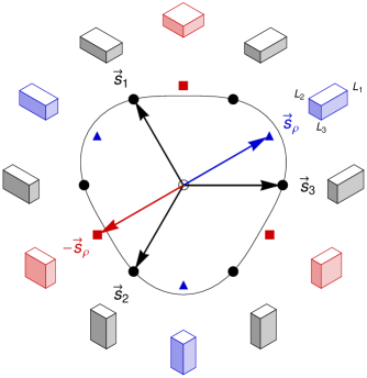
Figure 10: (Color online) The $d{-}1$-dimensional plane $\mathcal{B}$ of constant volume $L^{d}$ for $d=3$, viewed from the normal direction $(1,1,1)$. The origin at the center ($\circ$) is the cube with $\vec{b}=\vec{0}$, while the filled symbols are deformed systems as indicated by the pictures: The black points mark the directions $\pm\vec{s}_{\mu}$ with constant $L_{\mu}$ symmetric under permutation $\mathcal{P}$, Eq. (62). The blue arrow $\vec{s}_{\rho}$ ($\rho>1$) and the red arrow $-\vec{s}_{\rho}$ ($\rho<1$) mark the direction of the shape variation in terms of $\rho$ used in this work. The black curve sketches a line of constant $\Theta(x,\vec{b})$. Note that $\Theta(x,\vec{s}_{\rho})\neq\Theta(x,-\vec{s}_{\rho})$, as the shape and thus $\Theta$ is not symmetric under the transformation $\rho\to 1/\rho$, see also Fig. 7.

The stationarity of the excess free energy scaling function $\Theta(x,\rho)$ at $\rho=1$ can be derived for isotropic systems with arbitrary symmetric boundary conditions and in arbitrary dimensions $d$: We allow arbitrary shape changes of $f_{\mathrm{ex}}(T,L_{1},\ldots,L_{d})$ and write $L_{\mu}=e^{b_{\mu}}L$, so that Eq. (10) now reads

$$f_{\mathrm{ex}}(T,e^{b_{1}}L,\ldots,e^{b_{d}}L)\sim L^{-d}\Theta(x,\vec{b}),$$ (60)

under the condition

$$\sum_{\mu=1}^{d}b_{\mu}=0$$ (61)

defining the plane $\mathcal{B}$ with constant volume $L^{d}$. The symmetry under permutation of the $d$ lattice axes implies

$$\Theta(x,\vec{b})=\Theta(x,\mathcal{P}(\vec{b}))$$ (62)

with permutation operator $\mathcal{P}$. This symmetry holds if the boundary conditions in all directions are equal. Without loss of generality we now assume $d=3$, $b_{1}=0$ and vary the shape of the system along directions $2$ and $3$, i. e., $b_{2}=-b_{3}$, so that $\Theta(x,\epsilon\,\vec{s}_{1})=\Theta(x,-\epsilon\,\vec{s}_{1})$ with $\vec{s}_{1}=(0,1,-1)$ and real $\epsilon$. Hence $\Theta(x,\epsilon\,\vec{s}_{1})$ is an even function of $\epsilon$ and thus the directional derivative along $\vec{s}_{1}$ at the origin vanishes,

$$\left.\frac{\partial}{\partial\epsilon}\Theta(x,\epsilon\,\vec{s}_{1})\right|_{\epsilon=0}=0.$$ (63)

The same argument holds for the symmetric directions $\vec{s}_{2}=(-1,0,1)$ and $\vec{s}_{3}=(1,-1,0)$ (see Fig. 10). As the $d(d-1)/2$ vectors $\vec{s}_{\mu}$ form an (over)complete base in the $d{-}1$-dimensional plane $\mathcal{B}$, and all directional derivatives vanish at the origin $\vec{b}=\vec{0}$, we conclude that Eq. (63) holds for all directions $\vec{s}\in\mathcal{B}$. Hence Eq. (63) also holds for the special case $\vec{s}_{\rho}=(2/3,-1/3,-1/3)$ which is the direction of the shape variation used in this work (with $\rho=e^{\epsilon}$), if we set $L_{1}=L_{\perp}$ and $L_{2}=L_{3}=L_{\parallel}$. From this we conclude that Eq. (10) satisfies

$$\left.\frac{\partial}{\partial\rho}\Theta(x,\rho)\right|_{\rho=1}=0.$$ (64)

Note that these arguments can be extended to weakly anisotropic systems, while less is known in the strongly anisotropic case Hucht (2002); Burgsmüller et al. (2010).

Appendix B Proof of $\boldsymbol{\vartheta(0,1)=0}$ in the large-$\boldsymbol{n}$ limit

In this appendix we show for the large-$n$ limit Dohm (2009) that the finite-size scaling function of the thermodynamic Casimir force vanishes at bulk criticality in the case of a cubic system geometry $\rho=1$. To this end we start from the scaling function of the singular free energy per volume given by Dohm (Eq. (3) in Dohm (2009)), together with the self-consistency equation for the parameter $P(x_{\perp},\rho)$ at $x_{\perp}=0$,

$$P(0,\rho)=-4\pi\mathcal{G}_{1}(P(0,\rho)^{2},\rho),$$ (65)

and the functions $\mathcal{G}_{j}(P^{2},\rho)$ (Eq. (4) in Dohm (2009)). Introducing the parameter $\hat{P}(\rho)\equiv\rho^{\mu}P(0,\rho)$ and furthermore the integration variable $\hat{z}=\rho^{\delta}z$ in the integral $\mathcal{G}_{0}(P^{2},\rho)$, the value of the excess free energy scaling function $\Theta_{\perp}$ (see Eq. (6)) at bulk criticality can be cast in the form

$$\Theta_{\perp}(0,\rho)=\Delta_{\perp}(\rho)=\rho^{2}\Delta(\rho)$$ (66)

upon setting $\mu=-2/3$ and $\delta=4/3$, where $\Delta(\rho)$ is given by

$$\Delta(\rho) = -\frac{\hat{P}(\rho)^{3}}{12\pi}+\frac{1}{2}\int_{0}^{\infty}\frac{\mathrm{d}\hat{z}}{\hat{z}}\exp\!\left(-\frac{\hat{z}\hat{P}(\rho)^{2}}{4\pi^{2}}\right)$$ (67)

$$\times\Bigl{[}\left(\frac{\pi}{\hat{z}}\right)^{3/2}-K(\rho^{-4/3}\hat{z})K(\rho^{2/3}\hat{z})^{2}\Bigr{]}.$$

According to Eq. (18) one has

$$\vartheta_{\perp}(x_{\perp}=0,\rho=1)=-\Delta^{\prime}(1),$$ (68)

where the derivative of $\Delta(\rho)$ with respect to $\rho$ at $\rho=1$ becomes

$$\Delta^{\prime}(1)=-\frac{\hat{P}(1)\hat{P}^{\prime}(1)}{4\pi}\left[\hat{P}(1)+4\pi\mathcal{G}_{1}(\hat{P}(1)^{2},1)\right].$$ (69)

Since $\hat{P}(1)=P(0,1)$ is the solution to Eq. (65) at $\rho=1$, the expression in square brackets vanishes and thus $\Delta^{\prime}(1)=0$.

References

- Casimir (1948) H. B. G. Casimir, Proc. K. Ned. Akad. Wet., 51, 793 (1948).
- Lamoreaux (1997) S. K. Lamoreaux, Phys. Rev. Lett., 78, 5 (1997), Phys. Rev. Lett., 81, 5475 (1998) (Erratum), arXiv:1007.4276.
- Mohideen and Roy (1998) U. Mohideen and A. Roy, Phys. Rev. Lett., 81, 4549 (1998).
- Fisher and de Gennes (1978) M. E. Fisher and P.-G. de Gennes, C. R. Acad. Sci. Paris, Ser. B, 287, 207 (1978).
- Gambassi (2009) A. Gambassi, Journal of Physics: Conference Series, 161, 012037 (2009).
- Garcia and Chan (1999) R. Garcia and M. H. W. Chan, Phys. Rev. Lett., 83, 1187 (1999).
- Ganshin et al. (2006) A. Ganshin, S. Scheidemantel, R. Garcia, and M. H. W. Chan, Phys. Rev. Lett., 97, 075301 (2006).
- Fukuto et al. (2005) M. Fukuto, Y. F. Yano, and P. S. Pershan, Phys. Rev. Lett., 94, 135702 (2005).
- Hertlein et al. (2008) C. Hertlein, L. Helden, A. Gambassi, S. Dietrich, and C. Bechinger, Nature, 451, 172 (2008).
- Gambassi et al. (2009) A. Gambassi, A. Maciołek, C. Hertlein, U. Nellen, L. Helden, C. Bechinger, and S. Dietrich, Phys. Rev. E, 80, 061143 (2009).
- Garcia and Chan (2002) R. Garcia and M. H. W. Chan, Phys. Rev. Lett., 88, 086101 (2002).
- Krech and Dietrich (1992) M. Krech and S. Dietrich, Phys. Rev. A, 46, 1886 (1992).
- Krech (1994) M. Krech, Casimir Effect in Critical Systems (World Scientific, Singapore, 1994).
- Diehl et al. (2006) H. W. Diehl, D. Grüneberg, and M. A. Shpot, Europhys. Lett., 75, 241 (2006).
- Grüneberg and Diehl (2008) D. Grüneberg and H. W. Diehl, Phys. Rev. B, 77, 115409 (2008).
- Maciołek et al. (2007) A. Maciołek, A. Gambassi, and S. Dietrich, Phys. Rev. E, 76, 031124 (2007).
- Zandi et al. (2007) R. Zandi, A. Shackell, J. Rudnick, M. Kardar, and L. P. Chayes, Phys. Rev. E, 76, 030601 (2007).
- Li and Kardar (1991) H. Li and M. Kardar, Phys. Rev. Lett., 67, 3275 (1991).
- Li and Kardar (1992) H. Li and M. Kardar, Phys. Rev. A, 46, 6490 (1992).
- Kardar and Golestanian (1999) M. Kardar and R. Golestanian, Rev. Mod. Phys., 71, 1233 (1999).
- Zandi et al. (2004) R. Zandi, J. Rudnick, and M. Kardar, Phys. Rev. Lett., 93, 155302 (2004).
- Hucht (2007) A. Hucht, Phys. Rev. Lett., 99, 185301 (2007).
- Dantchev and Krech (2004) D. Dantchev and M. Krech, Phys. Rev. E, 69, 046119 (2004).
- Hasenbusch (2010) M. Hasenbusch, Phys. Rev. B, 81, 165412 (2010a), arXiv:0907.2847.
- Hasenbusch (2010) M. Hasenbusch, Phys. Rev. B, 82, 104425 (2010b), arXiv:1005.4749.
- Vasilyev et al. (2007) O. Vasilyev, A. Gambassi, A. Maciołek, and S. Dietrich, Europhys. Lett., 80, 60009 (2007).
- Hasenbusch (2009) M. Hasenbusch, J. Stat. Mech.: Theory Exp., P07031 (2009a), arXiv:0905.2096.
- Hasenbusch (2009) M. Hasenbusch, Phys. Rev. E, 80, 061120 (2009b), arXiv:0908.3582.
- Vasilyev et al. (2009) O. Vasilyev, A. Gambassi, A. Maciołek, and S. Dietrich, Phys. Rev. E, 79, 041142 (2009).
- Toldin and Dietrich (2010) F. P. Toldin and S. Dietrich, J. Stat. Mech.: Theory Exp., 2010, P11003 (2010).
- Dohm (2009) V. Dohm, Europhys. Lett., 86, 20001 (5pp) (2009).
- Privman (1990) V. Privman, in Finite Size Scaling and Numerical Simulation of Statistical Systems, edited by V. Privman (World Scientific, Singapore, 1990) Chap. 1.
- Note (1) Throughout this work, the symbol means “asymptotically equal” in the respective limit, , , keeping the scaling variables and fixed, i.\tmspace+.1667eme., .
- Campostrini et al. (1999) M. Campostrini, A. Pelissetto, P. Rossi, and E. Vicari, Phys. Rev. E, 60, 3526 (1999).
- Butera and Comi (2002) P. Butera and M. Comi, Phys. Rev. B, 65, 144431 (2002).
- Fisher (1971) M. E. Fisher, in Critical Phenomena, Proceedings of the 51st Enrico Fermi Summer School, Varenna, Italy, edited by M. S. Green (Academic Press, New York, 1971) pp. 73–98.
- Dantchev et al. (2006) D. Dantchev, H. W. Diehl, and D. Grüneberg, Phys. Rev. E, 73, 016131 (2006).
- Grüneberg and Hucht (2004) D. Grüneberg and A. Hucht, Phys. Rev. E, 69, 036104 (2004).
- Danchev (1998) D. M. Danchev, Phys. Rev. E, 58, 1455 (1998).
- Brankov et al. (2000) J. G. Brankov, D. M. Dantchev, and N. S. Tonchev, Theory of Critical Phenomena in Finite-Size Systems – Scaling and Quantum Effects (World Scientific, Singapore, 2000).
- Dantchev et al. (2003) D. Dantchev, M. Krech, and S. Dietrich, Phys. Rev. E, 67, 066120 (2003).
- Dantchev and Grüneberg (2009) D. Dantchev and D. Grüneberg, Phys. Rev. E, 79, 041103 (2009).
- Krech and Landau (1996) M. Krech and D. P. Landau, Phys. Rev. E, 53, 4414 (1996).
- Schmidt and Diehl (2008) F. M. Schmidt and H. W. Diehl, Phys. Rev. Lett., 101, 100601 (2008).
- Diehl and Grüneberg (2009) H. W. Diehl and D. Grüneberg, Nucl. Phys. B, 822, 517 (2009).
- Burgsmüller et al. (2010) M. Burgsmüller, H. W. Diehl, and M. A. Shpot, J. Stat. Mech.: Theory Exp., P11020 (2010).
- Bhanot et al. (1994) G. Bhanot, M. Creutz, I. Horvath, J. Lacki, and J. Weckel, Phys. Rev. E, 49, 2445 (1994).
- Feng and Blöte (2010) X. Feng and H. W. J. Blöte, Phys. Rev. E, 81, 031103 (2010).
- Arisue and Fujiwara (2003) H. Arisue and T. Fujiwara, Phys. Rev. E, 67, 066109 (2003), there is a typo in the 42th order term, the correct value appears in arXiv:hep-lat/0209002.
- Wolff (1989) U. Wolff, Phys. Rev. Lett., 62, 361 (1989).
- Deng and Blöte (2003) Y. Deng and H. W. J. Blöte, Phys. Rev. E, 68, 036125 (2003).
- Kitatani et al. (1996) H. Kitatani, M. Ohta, and N. Ito, J. Phys. Soc. Jpn., 65, 4050 (1996).
- Caselle and Hasenbusch (1996) M. Caselle and M. Hasenbusch, Nucl. Phys. B, 470, 435 (1996), ISSN 0550-3213.
- Krech (1997) M. Krech, Phys. Rev. E, 56, 1642 (1997).
- Note (2) At all quantities obey .
- Bachas (2007) C. P. Bachas, J. Phys A: Math. Theor., 40, 9089 (2007).
- Privman and Fisher (1983) V. Privman and M. E. Fisher, J. Stat. Phys., 33, 385 (1983).
- Mon (1985) K. K. Mon, Phys. Rev. Lett., 54, 2671 (1985).
- Ferdinand and Fisher (1969) A. E. Ferdinand and M. E. Fisher, Phys. Rev., 185, 832 (1969), there is a typo in Eq. (3.36), the term is missing.
- Kaufman (1949) B. Kaufman, Phys. Rev., 76, 1232 (1949).
- Wolfram Research, Inc. (2008) Wolfram Research, Inc., Mathematica V7.0, Champaign, Illinois (2008).
- Whittaker and Watson (1990) E. T. Whittaker and G. N. Watson, A Course in Modern Analysis, 4th ed. (Cambridge University Press, 1990).
- Rudnick et al. (2010) J. Rudnick, R. Zandi, A. Shackell, and D. Abraham, Phys. Rev. E, 82, 041118 (2010).
- Hucht (2002) A. Hucht, J. Phys A: Math. Gen., 35, L481 (2002).