Microlocal analysis of asymptotically hyperbolic and Kerr-de Sitter spaces

Abstract.

In this paper we develop a general, systematic, microlocal framework for the Fredholm analysis of non-elliptic problems, including high energy (or semiclassical) estimates, which is stable under perturbations. This framework, described in Section 2, resides on a compact manifold without boundary, hence in the standard setting of microlocal analysis.

Many natural applications arise in the setting of non-Riemannian b-metrics in the context of Melrose’s b-structures. These include asymptotically de Sitter-type metrics on a blow-up of the natural compactification, Kerr-de Sitter-type metrics, as well as asymptotically Minkowski metrics.

The simplest application is a new approach to analysis on Riemannian or Lorentzian (or indeed, possibly of other signature) conformally compact spaces (such as asymptotically hyperbolic or de Sitter spaces), including a new construction of the meromorphic extension of the resolvent of the Laplacian in the Riemannian case, as well as high energy estimates for the spectral parameter in strips of the complex plane. These results are also available in a follow-up paper which is more expository in nature, [54].

The appendix written by Dyatlov relates his analysis of resonances on exact Kerr-de Sitter space (which then was used to analyze the wave equation in that setting) to the more general method described here.

1. Introduction

In this paper we develop a general microlocal framework which in particular allows us to analyze the asymptotic behavior of solutions of the wave equation on asymptotically Kerr-de Sitter and Minkowski space-times, as well as the behavior of the analytic continuation of the resolvent of the Laplacian on so-called conformally compact spaces. This framework is non-perturbative, and works, in particular, for black holes, for relatively large angular momenta (the restrictions come purely from dynamics, and not from methods of analysis of PDE), and also for perturbations of Kerr-de Sitter space, where ‘perturbation’ is only relevant to the extent that it guarantees that the relevant structures are preserved. In the context of analysis on conformally compact spaces, our framework establishes a Riemannian-Lorentzian duality; in this duality the spaces of different signature are smooth continuations of each other across a boundary at which the differential operator we study has some radial points in the sense of microlocal analysis.

Since it is particularly easy to state, and only involves Riemannian geometry, we start by giving a result on manifolds with even conformally compact metrics. These are Riemannian metrics $g_{0}$ on the interior of a compact manifold with boundary $X_{0}$ such that near the boundary $Y$, with a product decomposition nearby and a defining function $x$, they are of the form

$$g_{0}=\frac{dx^{2}+h}{x^{2}},$$

where $h$ is a family of metrics on $\partial X_{0}$ depending on $x$ in an even manner, i.e. only even powers of $x$ show up in the Taylor series. (There is a much more natural way to phrase the evenness condition, see [28, Definition 1.2].) We also write $X_{0,\mathrm{even}}$ for the manifold $X_{0}$ when the smooth structure has been changed so that $x^{2}$ is a boundary defining function; thus, a smooth function on $X_{0}$ is even if and only if it is smooth when regarded as a function on $X_{0,\mathrm{even}}$. The analytic continuation of the resolvent in this category (but without the evenness condition) was obtained by Mazzeo and Melrose [37], with possibly some essential singularities at pure imaginary half-integers as noticed by Borthwick and Perry [6]. Using methods of Graham and Zworski [26], Guillarmou [28] showed that for even metrics the latter do not exist, but generically they do exist for non-even metrics. Further, if the manifold is actually asymptotic to hyperbolic space (note that hyperbolic space is of this form in view of the Poincaré model), Melrose, Sá Barreto and Vasy [41] showed high energy resolvent estimates in strips around the real axis via a parametrix construction; these are exactly the estimates that allow expansions for solutions of the wave equation in terms of resonances. Estimates just on the real axis were obtained by Cardoso and Vodev for more general conformal infinities [7, 57]. One implication of our methods is a generalization of these results.

Below $\dot{\mathcal{C}}^{\infty}(X_{0})$ denotes ‘Schwartz functions’ on $X_{0}$, i.e. $\mathcal{C}^{\infty}$ functions vanishing with all derivatives at $\partial X_{0}$, and $\mathcal{C}^{-\infty}(X_{0})$ is the dual space of ‘tempered distributions’ (these spaces are naturally identified for $X_{0}$ and $X_{0,\mathrm{even}}$), while $H^{s}(X_{0,\mathrm{even}})$ is the standard Sobolev space on $X_{0,\mathrm{even}}$ (corresponding to extension across the boundary, see e.g. [32, Appendix B], where these are denoted by $\bar{H}^{s}(X_{0,\mathrm{even}}^{\circ})$) and $H^{s}_{h}(X_{0,\mathrm{even}})$ is the standard semiclassical Sobolev space, so for $h>0$ fixed this is the same as $H^{s}(X_{0,\mathrm{even}})$; see [17, 21].

Theorem.

(See Theorem 4.3 for the full statement.) Suppose that $X_{0}$ is an $(n-1)$-dimensional manifold with boundary $Y$ with an even Riemannian conformally compact metric $g_{0}$. Then the inverse of

$$\Delta_{g_{0}}-\left(\frac{n-2}{2}\right)^{2}-\sigma^{2},$$

written as $\mathcal{R}(\sigma):L^{2}\to L^{2}$, has a meromorphic continuation from $\operatorname{Im}\sigma\gg 0$ to $\mathbb{C}$,

$$\mathcal{R}(\sigma):\dot{\mathcal{C}}^{\infty}(X_{0})\to\mathcal{C}^{-\infty}(X_{0}),$$

with poles with finite rank residues. If in addition $(X_{0},g_{0})$ is non-trapping, then non-trapping estimates hold in every strip $|\operatorname{Im}\sigma|<C$, $|\operatorname{Re}\sigma|\gg 0$: for $s>\frac{1}{2}+C$,

(1.1) $$\|x^{-(n-2)/2+\imath\sigma}\mathcal{R}(\sigma)f\|_{H^{s}_{|\sigma|^{-1}}(X_{0,\mathrm{even}})}\leq\tilde{C}|\sigma|^{-1}\|x^{-(n+2)/2+\imath\sigma}f\|_{H^{s-1}_{|\sigma|^{-1}}(X_{0,\mathrm{even}})}.$$

If $f$ has compact support in $X_{0}^{\circ}$, the $s-1$ norm on $f$ can be replaced by the $s-2$ norm.

Further, as stated in Theorem 4.3, the resolvent is semiclassically outgoing with a loss of $h^{-1}$, in the sense of recent results of Datchev and Vasy [15] and [16]. This means that for mild trapping (where, in a strip near the spectrum, one has polynomially bounded resolvent for a compactly localized version of the trapped model) one obtains resolvent bounds of the same kind as for the above-mentioned trapped models, and lossless estimates microlocally away from the trapping. In particular, one obtains logarithmic losses compared to non-trapping on the spectrum for hyperbolic trapping in the sense of [60, Section 1.2], and polynomial losses in strips, since for the compactly localized model this was recently shown by Wunsch and Zworski [60].

For conformally compact spaces, without using wave propagation as motivation, our method is to change the smooth structure, replacing $x$ by $\mu=x^{2}$, conjugate the operator by an appropriate weight as well as remove a vanishing factor of $\mu$, and show that the new operator continues smoothly and non-degenerately (in an appropriate sense) across $\mu=0$, i.e. $Y$, to a (non-elliptic) problem which we can analyze utilizing by now almost standard tools of microlocal analysis. These steps are reflected in the form of the estimate (1.1); $\mu$ shows up in the evenness, conjugation due to the presence of $x^{-n/2+\imath\sigma}$, and the two halves of the vanishing factor of $\mu$ being removed in $x^{\pm 1}$ on the left and right hand sides. This approach is explained in full detail in the more expository and self-contained follow-up article, [54].

However, it is useful to think of a wave equation motivation — then $(n-1)$-dimensional hyperbolic space shows up (essentially) as a model at infinity inside a backward light cone from a fixed point $q_{+}$ at future infinity on $n$-dimensional de Sitter space $\hat{M}$, see [53, Section 7], where this was used to construct the Poisson operator. More precisely, the light cone is singular at $q_{+}$, so to desingularize it, consider $[\hat{M};\{q_{+}\}]$. After a Mellin transform in the defining function of the front face; the model continues smoothly across the light cone $Y$ inside the front face of $[\hat{M};\{q_{+}\}]$. The inside of the light cone corresponds to $(n-1)$-dimensional hyperbolic space (after conjugation, etc.) while the exterior is (essentially) $(n-1)$-dimensional de Sitter space; $Y$ is the ‘boundary’ separating them. Here $Y$ should be thought of as the event horizon in black hole terms (there is nothing more to event horizons in terms of local geometry!).

The resulting operator $P_{\sigma}$ has radial points at the conormal bundle $N^{*}Y\setminus o$ of $Y$ in the sense of microlocal analysis, i.e. the Hamilton vector field is radial at these points, i.e. is a multiple of the generator of dilations of the fibers of the cotangent bundle there. However, tools exist to deal with these, going back to Melrose’s geometric treatment of scattering theory on asymptotically Euclidean spaces [39]. Note that $N^{*}Y\setminus o$ consists of two components, $\Lambda_{+}$, resp. $\Lambda_{-}$, and in $S^{*}X=(T^{*}X\setminus o)/\mathbb{R}^{+}$ the images, $L_{+}$, resp. $L_{-}$, of these are sinks, resp. sources, for the Hamilton flow. At $L_{\pm}$ one has choices regarding the direction one wants to propagate estimates (into or out of the radial points), which directly correspond to working with strong or weak Sobolev spaces. For the present problem, the relevant choice is propagating estimates away from the radial points, thus working with the ‘good’ Sobolev spaces (which can be taken to have as positive order as one wishes; there is a minimum amount of regularity imposed by our choice of propagation direction, cf. the requirement $s>\frac{1}{2}+C$ above (1.1)). All other points are either elliptic, or real principal type. It remains to either deal with the non-compactness of the ‘far end’ of the $(n-1)$-dimensional de Sitter space — or instead, as is indeed more convenient when one wants to deal with more singular geometries, adding complex absorbing potentials, in the spirit of works of Nonnenmacher and Zworski [44] and Wunsch and Zworski [60]. In fact, the complex absorption could be replaced by adding a space-like boundary, see Remark 2.5, but for many microlocal purposes complex absorption is more desirable, hence we follow the latter method. However, crucially, these complex absorbing techniques (or the addition of a space-like boundary) already enter in the non-semiclassical problem in our case, as we are in a non-elliptic setting.

One can reverse the direction of the argument and analyze the wave equation on an $(n-1)$-dimensional even asymptotically de Sitter space $X_{0}^{\prime}$ by extending it across the boundary, much like the the Riemannian conformally compact space $X_{0}$ is extended in this approach. Then, performing microlocal propagation in the opposite direction, which amounts to working with the adjoint operators that we already need in order to prove existence of solutions for the Riemannian spaces, we obtain existence, uniqueness and structure results for asymptotically de Sitter spaces, recovering a large part of the results of [53]. Here we only briefly indicate this method of analysis in Remark 4.6.

In other words, we establish a Riemannian-Lorentzian duality, that will have counterparts both in the pseudo-Riemannian setting of higher signature and in higher rank symmetric spaces, though in the latter the analysis might become more complicated. Note that asymptotically hyperbolic and de Sitter spaces are not connected by a ‘complex rotation’ (in the sense of an actual deformation); they are smooth continuations of each other in the sense we just discussed.

To emphasize the simplicity of our method, we list all of the microlocal techniques (which are relevant both in the classical and in the semiclassical setting) that we use on a compact manifold without boundary; in all cases only microlocal Sobolev estimates matter (not parametrices, etc.):

1. Microlocal elliptic regularity.

2. Real principal type propagation of singularities.

3. Rough analysis at a Lagrangian invariant under the Hamilton flow which roughly behaves like a collection of radial points, though the internal structure does not matter, in the spirit of [39, Section 9].

4. Complex absorbing ‘potentials’ in the spirit of [44] and [60].

These are almost ‘off the shelf’ in terms of modern microlocal analysis, and thus our approach, from a microlocal perspective, is quite simple. We use these to show that on the continuation across the boundary of the conformally compact space we have a Fredholm problem, on a perhaps slightly exotic function space, which however is (perhaps apart from the complex absorption) the simplest possible coisotropic function space based on a Sobolev space, with order dictated by the radial points. Also, we propagate the estimates along bicharacteristics in different directions depending on the component $\Sigma_{\pm}$ of the characteristic set under consideration; correspondingly the sign of the complex absorbing ‘potential’ will vary with $\Sigma_{\pm}$, which is perhaps slightly unusual. However, this is completely parallel to solving the standard Cauchy, or forward, problem for the wave equation, where one propagates estimates in opposite directions relative to the Hamilton vector field in the two components.

The complex absorption we use modifies the operator $P_{\sigma}$ outside $X_{0,\mathrm{even}}$. However, while $(P_{\sigma}-\imath Q_{\sigma})^{-1}$ depends on $Q_{\sigma}$, its behavior on $X_{0,\mathrm{even}}$, and even near $X_{0,\mathrm{even}}$, is independent of this choice; see the proof of Proposition 4.2 for a detailed explanation. In particular, although $(P_{\sigma}-\imath Q_{\sigma})^{-1}$ may have resonances other than those of $\mathcal{R}(\sigma)$, the resonant states of these additional resonances are supported outside $X_{0,\mathrm{even}}$, hence do not affect the singular behavior of the resolvent in $X_{0,\mathrm{even}}$. In the setting of Kerr-de Sitter space an analogous role is played by semiclassical versions of the standard energy estimate; this is stated in Subsection 3.3.

While the results are stated for the scalar equation, analogous results hold for operators on natural vector bundles, such as the Laplacian on differential forms. This is so because the results work if the principal symbol of the extended problem is scalar with the demanded properties, and the imaginary part of the subprincipal symbol is either scalar at the ‘radial sets’, or instead satisfies appropriate estimates (as an endomorphism of the pull-back of the vector bundle to the cotangent bundle) at this location; see Remark 2.1. The only change in terms of results on asymptotically hyperbolic spaces is that the threshold $(n-2)^{2}/4$ is shifted; in terms of the explicit conjugation of Subsection 4.9 this is so because of the change in the first order term in (4.29).

While here we mostly consider conformally compact Riemannian or Lorentzian spaces (such as hyperbolic space and de Sitter space) as appropriate boundary values (Mellin transform) of a blow-up of de Sitter space of one higher dimension, they also show up as a boundary value of Minkowski space. This is related to Wang’s work on b-regularity [59], though Wang worked on a blown up version of Minkowski space-time; she also obtained her results for the (non-linear) Einstein equation there. It is also related to the work of Fefferman and Graham [22] on conformal invariants by extending an asymptotically hyperbolic manifold to Minkowski-type spaces of one higher dimension. We discuss asymptotically Minkowski spaces briefly in Section 5.

Apart from trapping — which is well away from the event horizons for black holes that do not rotate too fast — the microlocal structure on de Sitter space is exactly the same as on Kerr-de Sitter space, or indeed Kerr space near the event horizon. (Kerr space has a Minkowski-type end as well; although Minkowski space also fits into our framework, it does so a different way than Kerr at the event horizon, so the result there is not immediate; see the comments below.) This is to be understood as follows: from the perspective we present here (as opposed to the perspective of [53]), the tools that go into the analysis of de Sitter space-time suffice also for Kerr-de Sitter space, and indeed a much wider class, apart from the need to deal with trapping. The trapping itself was analyzed by Wunsch and Zworski [60]; their work fits immediately with our microlocal methods. Phenomena such as the ergosphere are mere shadows of dynamics in the phase space which is barely changed, but whose projection to the base space (physical space) undergoes serious changes. It is thus of great value to work microlocally, although it is certainly possible that for some non-linear purposes it is convenient to rely on physical space to the maximum possible extent, as was done in the recent (linear) works of Dafermos and Rodnianski [13, 14].

Below we state theorems for Kerr-de Sitter space time. However, it is important to note that all of these theorems have analogues in the general microlocal framework discussed in Section 2. In particular, analogous theorems hold on conjugated, re-weighted, and even versions of Laplacians on conformally compact spaces (of which one example was stated above as a theorem), and similar results apply on ‘asymptotically Minkowski’ spaces, with the slight twist that it is adjoints of operators considered here that play the direct role there.

We now turn to Kerr-de Sitter space-time and give some history. In exact Kerr-de Sitter space and for small angular momentum, Dyatlov [20, 19] has shown exponential decay to constants, even across the event horizon. This followed earlier work of Melrose, Sá Barreto and Vasy [40], where this was shown up to the event horizon in de Sitter-Schwarzschild space-times or spaces strongly asymptotic to these (in particular, no rotation of the black hole is allowed), and of Dafermos and Rodnianski in [11] who had shown polynomial decay in this setting. These in turn followed up pioneering work of Sá Barreto and Zworski [47] and Bony and Häfner [5] who studied resonances and decay away from the event horizon in these settings. (One can solve the wave equation explicitly on de Sitter space using special functions, see [45] and [61]; on asymptotically de Sitter spaces the forward fundamental solution was constructed as an appropriate Lagrangian distribution by Baskin [1].)

Also, polynomial decay on Kerr space was shown recently by Tataru and Tohaneanu [50, 49] and Dafermos and Rodnianski [13, 14], after pioneering work of Kay and Wald in [33] and [58] in the Schwarzschild setting. (There was also recent work by Marzuola, Metcalf, Tataru and Tohaneanu [36] on Strichartz estimates, and by Donninger, Schlag and Soffer [18] on $L^{\infty}$ estimates on Schwarzschild black holes, following $L^{\infty}$ estimates of Dafermos and Rodnianski [12, 10], of Blue and Soffer [4] on non-rotating charged black holes giving $L^{6}$ estimates, and Finster, Kamran, Smoller and Yau [23, 24] on Dirac waves on Kerr.) While some of these papers employ microlocal methods at the trapped set, they are mostly based on physical space where the phenomena are less clear than in phase space (unstable tools, such as separation of variables, are often used in phase space though). We remark that Kerr space is less amenable to immediate microlocal analysis to attack the decay of solutions of the wave equation due to the singular/degenerate behavior at zero frequency, which will be explained below briefly. This is closely related to the behavior of solutions of the wave equation on Minkowski space-times. Although our methods also deal with Minkowski space-times, this holds in a slightly different way than for de Sitter (or Kerr-de Sitter) type spaces at infinity, and combining the two ingredients requires some additional work. On perturbations of Minkowski space itself, the full non-linear analysis was done in the path-breaking work of Christodoulou and Klainerman [9], and Lindblad and Rodnianski simplified the analysis [34, 35], Bieri [2, 3] succeeded in relaxing the decay conditions, while Wang [59] obtained additional, b-type, regularity as already mentioned. Here we only give a linear result, but hopefully its simplicity will also shed new light on the non-linear problem.

As already mentioned, a microlocal study of the trapping in Kerr or Kerr-de Sitter was performed by Wunsch and Zworski in [60]. This is particularly important to us, as this is the only part of the phase space which does not fit directly into a relatively simple microlocal framework. Our general method is to use microlocal analysis to understand the rest of the phase space (with localization away from trapping realized via a complex absorbing potential), then use the gluing result of Datchev and Vasy [15] to obtain the full result.

Slightly more concretely, in the appropriate (partial) compactification of space-time, near the boundary of which space-time has the form $X_{\delta}\times[0,\tau_{0})_{\tau}$, where $X_{\delta}$ denotes an extension of the space-time across the event horizon. Thus, there is a manifold with boundary $X_{0}$, whose boundary $Y$ is the event horizon, such that $X_{0}$ is embedded into $X_{\delta}$, a (non-compact) manifold without boundary. We write $X_{+}=X_{0}^{\circ}$ for ‘our side’ of the event horizon and $X_{-}=X_{\delta}\setminus X_{0}$ for the ‘far side’. Then the Kerr or Kerr-de Sitter d’Alembertians are b-operators in the sense of Melrose [43] that extend smoothly across the event horizon $Y$. Recall that in the Riemannian setting, b-operators are usually called ‘cylindrical ends’, see [43] for a general description; here the form at the boundary (i.e. ‘infinity’) is similar, modulo ellipticity (which is lost). Our results hold for small smooth perturbations of Kerr-de Sitter space in this b-sense. Here the role of ‘perturbations’ is simply to ensure that the microlocal picture, in particular the dynamics, has not changed drastically. Although b-analysis is the right conceptual framework, we mostly work with the Mellin transform, hence on manifolds without boundary, so the reader need not be concerned about the lack of familiarity with b-methods. However, we briefly discuss the basics in Section 3.

We immediately Mellin transform in the defining function of the boundary (which is temporal infinity, though is not space-like everywhere) — in Kerr and Kerr-de Sitter spaces this is operation is ‘exact’, corresponding to $\tau\partial_{\tau}$ being a Killing vector field, i.e. is not merely at the level of normal operators, but this makes little difference (i.e. the general case is similarly treatable). After this transform we get a family of operators that e.g. in de Sitter space is elliptic on $X_{+}$, but in Kerr space ellipticity is lost there. We consider the event horizon as a completely artificial boundary even in the de Sitter setting, i.e. work on a manifold that includes a neighborhood of $X_{0}=\overline{X_{+}}$, hence a neighborhood of the event horizon $Y$.

As already mentioned, one feature of these space-times is some relatively mild trapping in $X_{+}$; this only plays a role in high energy (in the Mellin parameter, $\sigma$), or equivalently semiclassical (in $h=|\sigma|^{-1}$) estimates. We ignore a (semiclassical) microlocal neighborhood of the trapping for a moment; we place an absorbing ‘potential’ there. Another important feature of the space-times is that they are not naturally compact on the ‘far side’ of the event horizon (inside the black hole), i.e. $X_{-}$, and bicharacteristics from the event horizon (classical or semiclassical) propagate into this region. However, we place an absorbing ‘potential’ (a second order operator) there to annihilate such phenomena which do not affect what happens on ‘our side’ of the event horizon, $X_{+}$, in view of the characteristic nature of the latter. This absorbing ‘potential’ could easily be replaced by a space-like boundary, in the spirit of introducing a boundary $t=t_{1}$, where $t_{1}>t_{0}$, when one solves the Cauchy problem from $t_{0}$ for the standard wave equation; note that such a boundary does not affect the solution of the equation in $[t_{0},t_{1}]_{t}$. Alternatively, if $X_{-}$ has a well-behaved infinity, such as in de Sitter space, the analysis could be carried out more globally. However, as we wish to emphasize the microlocal simplicity of the problem, we do not touch on these issues.

All of our results are in a general setting of microlocal analysis explained in Section 2, with the Mellin transform and Lorentzian connection explained in Section 3. However, for the convenience of the reader here we state the results for perturbations of Kerr-de Sitter spaces. We refer to Section 6 for details. First, the general assumption is that

$P_{\sigma}$, $\sigma\in\mathbb{C}$, is either the Mellin transform of the d’Alembertian ${\square}_{g}$ for a Kerr-de Sitter spacetime, or more generally the Mellin transform of the normal operator of the d’Alembertian ${\square}_{g}$ for a small perturbation, in the sense of b-metrics, of such a Kerr-de Sitter space-time;

see Section 3 for an explanation of these concepts. Note that for such perturbations the usual ‘time’ Killing vector field (denoted by $\partial_{\tilde{t}}$ in Section 6; this is indeed time-like in $X_{+}\times[0,\epsilon)_{\tilde{t}}$ sufficiently far from $\partial X_{+}$) is no longer Killing. Our results on these space-times are proved by showing that the hypotheses of Section 2 are satisfied. We show this in general (under the conditions (6.2), which corresponds to $0<\frac{9}{4}\Lambda r_{s}^{2}<1$ in de Sitter-Schwarzschild spaces, and (6.12), which corresponds to the lack of classical trapping in $X_{+}$; see Section 6), except where semiclassical dynamics matters. As in the analysis of Riemannian conformally compact spaces, we use a complex absorbing operator $Q_{\sigma}$; this means that its principal symbol in the relevant (classical, or semiclassical) sense has the correct sign on the characteristic set; see Section 2.

When semiclassical dynamics does matter, the non-trapping assumption with an absorbing operator $Q_{\sigma}$, $\sigma=h^{-1}z$, is

in both the forward and backward directions, the bicharacteristics from any point in the semiclassical characteristic set of $P_{\sigma}$ either enter the semiclassical elliptic set of $Q_{\sigma}$ at some finite time, or tend to $L_{\pm}$;

see Definition 2.13. Here, as in the discussion above, $L_{\pm}$ are two components of the image of $N^{*}Y\setminus o$ in $S^{*}X$. (As $L_{+}$ is a sink while $L_{-}$ is a source, even semiclassically, outside $L_{\pm}$ the ‘tending’ can only happen in the forward, resp. backward, directions.) Note that the semiclassical non-trapping assumption (in the precise sense used below) implies a classical non-trapping assumption, i.e. the analogous statement for classical bicharacteristics, i.e. those in $S^{*}X$. It is important to keep in mind that the classical non-trapping assumption can always be satisfied with $Q_{\sigma}$ supported in $X_{-}$, far from $Y$.

In our first result in the Kerr-de Sitter type setting, to keep things simple, we ignore semiclassical trapping via the use of $Q_{\sigma}$; this means that $Q_{\sigma}$ will have support in $X_{+}$. However, in $X_{+}$, $Q_{\sigma}$ only matters in the semiclassical, or high energy, regime, and only for (almost) real $\sigma$. If the black hole is rotating relatively slowly, e.g. $\alpha$ satisfies the bound (6.22), the (semiclassical) trapping is always far from the event horizon, and one can make $Q_{\sigma}$ supported away from there. Also, the Klein-Gordon parameter $\lambda$ below is ‘free’ in the sense that it does not affect any of the relevant information in the analysis (principal and subprincipal symbol; see below). Thus, we drop it in the following theorems for simplicity.

Theorem 1.1.

Let $Q_{\sigma}$ be an absorbing formally self-adjoint operator such that the semiclassical non-trapping assumption holds. Let $\sigma_{0}\in\mathbb{C}$, and

$$\begin{split}&\mathcal{X}^{s}=\{u\in H^{s}:\ (P_{\sigma_{0}}-\imath Q_{\sigma_{0}})u\in H^{s-1}\},\ \mathcal{Y}^{s}=H^{s-1},\\ &\qquad\|u\|_{\mathcal{X}^{s}}^{2}=\|u\|_{H^{s}}^{2}+\|(P_{\sigma_{0}}-\imath Q_{\sigma_{0}})u\|^{2}_{H^{s-1}}.\end{split}$$

Let $\beta_{\pm}>0$ be given by the geometry at conormal bundle of the black hole ($-$), resp. de Sitter ($+$) event horizons, see Subsection 6.1, and in particular (LABEL:eq:subpr-Kerr). For $s\in\mathbb{R}$, let $\beta=\max(\beta_{+},\beta_{-})$ if $s\geq 1/2$, $\beta=\min(\beta_{+},\beta_{-})$ if $s<1/2$. Then, for $\lambda\in\mathbb{C}$,

$$P_{\sigma}-\imath Q_{\sigma}-\lambda:\mathcal{X}^{s}\to\mathcal{Y}^{s}$$

is an analytic family of Fredholm operators on

(1.2) $$\mathbb{C}_{s}=\{\sigma\in\mathbb{C}:\ \operatorname{Im}\sigma>\beta^{-1}(1-2s)\}$$

and has a meromorphic inverse,

$$R(\sigma)=(P_{\sigma}-\imath Q_{\sigma}-\lambda)^{-1},$$

which is holomorphic in an upper half plane, $\operatorname{Im}\sigma>C$. Moreover, given any $C^{\prime}>0$, there are only finitely many poles in $\operatorname{Im}\sigma>-C^{\prime}$, and the resolvent satisfies non-trapping estimates there, which e.g. with $s=1$ (which might need a reduction in $C^{\prime}>0$) take the form

$$\|R(\sigma)f\|_{L^{2}}^{2}+|\sigma|^{-2}\|dR(\sigma)\|_{L^{2}}^{2}\leq C^{\prime\prime}|\sigma|^{-2}\|f\|_{L^{2}}^{2}.$$

The analogous result also holds on Kerr space-time if we suppress the Euclidean end by a complex absorption.

Dropping the semiclassical absorption in $X_{+}$, i.e. if we make $Q_{\sigma}$ supported only in $X_{-}$, we have

Theorem 1.2.

Let $P_{\sigma}$, $\beta$, $\mathbb{C}_{s}$ be as in Theorem 1.1, and let $Q_{\sigma}$ be an absorbing formally self-adjoint operator supported in $X_{-}$ which is classically non-trapping. Let $\sigma_{0}\in\mathbb{C}$, and

$$\mathcal{X}^{s}=\{u\in H^{s}:\ (P_{\sigma_{0}}-\imath Q_{\sigma_{0}})u\in H^{s-1}\},\ \mathcal{Y}^{s}=H^{s-1},$$

with

$$\|u\|_{\mathcal{X}^{s}}^{2}=\|u\|_{H^{s}}^{2}+\|\tilde{P}u\|^{2}_{H^{s-1}}.$$

Then,

$$P_{\sigma}-\imath Q_{\sigma}:\mathcal{X}^{s}\to\mathcal{Y}^{s}$$

is an analytic family of Fredholm operators on $\mathbb{C}_{s}$, and has a meromorphic inverse,

$$R(\sigma)=(P_{\sigma}-\imath Q_{\sigma})^{-1},$$

which for any $\epsilon>0$ is holomorphic in a translated sector in the upper half plane, $\operatorname{Im}\sigma>C+\epsilon|\operatorname{Re}\sigma|$. The poles of the resolvent are called resonances. In addition, taking $s=1$ for instance, $R(\sigma)$ satisfies non-trapping estimates, e.g. with $s=1$,

$$\|R(\sigma)f\|_{L^{2}}^{2}+|\sigma|^{-2}\|dR(\sigma)\|_{L^{2}}^{2}\leq C^{\prime}|\sigma|^{-2}\|f\|_{L^{2}}^{2}$$

in such a translated sector.

It is in this setting that $Q_{\sigma}$ could be replaced by working on a manifold with boundary, with the boundary being space-like, essentially as a time level set mentioned above, since it is supported in $X_{-}$.

Now we make the assumption that the only semiclassical trapping is due to hyperbolic trapping with trapped set $\Gamma_{z}$, $\sigma=h^{-1}z$, with hyperbolicity understood as in the ‘Dynamical Hypotheses’ part of [60, Section 1.2], i.e.

in both the forward and backward directions, the bicharacteristics from any point in the semiclassical characteristic set of $P_{\sigma}$ either enter the semiclassical elliptic set of $Q_{\sigma}$ at some finite time, or tend to $L_{\pm}\cup\Gamma_{z}$.

We remark that just hyperbolicity of the trapped set suffices for the results of [60], see Section 1.2 of that paper; however, if one wants stability of the results under perturbations, one needs to assume that $\Gamma_{z}$ is normally hyperbolic. We refer to [60, Section 1.2] for a discussion of these concepts. We show in Section 6 that for black holes satisfying (6.22) (so the angular momentum can be comparable to the mass) the operators $Q_{\sigma}$ can be chosen so that they are supported in $X_{-}$ (even quite far from $Y$) and the hyperbolicity requirement is satisfied. Further, we also show that for slowly rotating black holes the trapping is normally hyperbolic. Moreover, the (normally) hyperbolic trapping statement is purely in Hamiltonian dynamics, not regarding PDEs. It might be known for an even larger range of rotation speeds, but the author is not aware of this.

Under this assumption, one can combine Theorem 1.1 with the results of Wunsch and Zworski [60] about hyperbolic trapping and the gluing results of Datchev and Vasy [15] to obtain a better result for the merely spatially localized problem, Theorem 1.2:

Theorem 1.3.

Let $P_{\sigma}$, $Q_{\sigma}$, $\beta$, $\mathbb{C}_{s}$, $\mathcal{X}^{s}$ and $\mathcal{Y}^{s}$ be as in Theorem 1.2, and assume that the only semiclassical trapping is due to hyperbolic trapping. Then,

$$P_{\sigma}-\imath Q_{\sigma}:\mathcal{X}^{s}\to\mathcal{Y}^{s}$$

is an analytic family of Fredholm operators on $\mathbb{C}_{s}$, and has a meromorphic inverse,

$$R(\sigma)=(P_{\sigma}-\imath Q_{\sigma})^{-1},$$

which is holomorphic in an upper half plane, $\operatorname{Im}\sigma>C$. Moreover, there exists $C^{\prime}>0$ such that there are only finitely many poles in $\operatorname{Im}\sigma>-C^{\prime}$, and the resolvent satisfies polynomial estimates there as $|\sigma|\to\infty$, $|\sigma|^{\varkappa}$, for some $\varkappa>0$, compared to the non-trapping case, with merely a logarithmic loss compared to non-trapping for real $\sigma$, e.g. with $s=1$:

$$\|R(\sigma)f\|_{L^{2}}^{2}+|\sigma|^{-2}\|dR(\sigma)\|_{L^{2}}^{2}\leq C^{\prime\prime}|\sigma|^{-2}(\log|\sigma|)^{2}\|f\|_{L^{2}}^{2}.$$

Farther, there are approximate lattices of poles generated by the trapping, as studied by Sá Barreto and Zworski in [47], and further by Bony and Häfner in [5], in the exact De Sitter-Schwarzschild and Schwarzschild settings, and in ongoing work by Dyatlov in the exact Kerr-de Sitter setting.

Theorem 1.3 immediately and directly gives the asymptotic behavior of solutions of the wave equation across the event horizon. Namely, the asymptotics of the wave equation depends on the finite number of resonances; their precise behavior depends on specifics of the space-time, i.e. on these resonances. This is true even in arbitrarily regular b-Sobolev spaces – in fact, the more decay we want to show, the higher Sobolev spaces we need to work in. Thus, a forteriori, this gives $L^{\infty}$ estimates. We state this formally as a theorem in the simplest case of slow rotation; in the general case one needs to analyze the (finite!) set of resonances along the reals to obtain such a conclusion, and for the perturbation part also to show normal hyperbolicity (which we only show for slow rotation):

Theorem 1.4.

Let $M_{\delta}$ be the partial compactification of Kerr-de Sitter space as in Section 6, with $\tau$ the boundary defining function. Suppose that $g$ is either a slowly rotating Kerr-de Sitter metric, or a small perturbation as a symmetric bilinear form on ${}^{{\mathrm{b}}}TM_{\delta}$. Then there exist $C^{\prime}>0$, $\varkappa>0$ such that for $0<\epsilon<C^{\prime}$ and $s>(1+\beta\epsilon)/2$ solutions of ${\square}_{g}u=f$ with $f\in\tau^{\epsilon}H^{s-1+\varkappa}_{{\mathrm{b}}}(M_{\delta})$ vanishing in $\tau>\tau_{0}$, and with $u$ vanishing in $\tau>\tau_{0}$, satisfy that for some constant $c_{0}$,

$$u-c_{0}\in\tau^{\epsilon}H^{s}_{{\mathrm{b}},\mathrm{loc}}(M_{\delta}).$$

Here the norms of both $c_{0}$ in $\mathbb{C}$ and $u-c_{0}$ in $\tau^{\epsilon}H^{s}_{{\mathrm{b}},\mathrm{loc}}(M_{\delta^{\prime}})$ are bounded by that of $f$ in $\tau^{\epsilon}H^{s-1+\varkappa}_{{\mathrm{b}}}(M_{\delta})$ for $\delta^{\prime}<\delta$.

More generally, if $g$ is a Kerr-de Sitter metric with hyperbolic trapping, then there exist $C^{\prime}>0$, $\varkappa>0$ such that for $0<\ell<C^{\prime}$ and $s>(1+\beta\ell)/2$ solutions of ${\square}_{g}u=f$ with $f\in\tau^{\ell}H^{s-1+\varkappa}_{{\mathrm{b}}}(M_{\delta})$ vanishing in $\tau>\tau_{0}$, and with $u$ vanishing in $\tau>\tau_{0}$, satisfy that for some $a_{j\kappa}\in\mathcal{C}^{\infty}(X_{\delta})$ (which are resonant states) and $\sigma_{j}\in\mathbb{C}$ (which are the resonances),

$$u^{\prime}=u-\sum_{j}\sum_{\kappa\leq m_{j}}\tau^{\imath\sigma_{j}}(\log|\tau|)^{\kappa}a_{j\kappa}\in\tau^{\ell}H^{s}_{{\mathrm{b}},\mathrm{loc}}(M_{\delta}).$$

Here the (semi)norms of both $a_{j\kappa}$ in $\mathcal{C}^{\infty}(X_{\delta^{\prime}})$ and $u^{\prime}$ in $\tau^{\ell}H^{s}_{{\mathrm{b}},\mathrm{loc}}(M_{\delta^{\prime}})$ are bounded by that of $f$ in $\tau^{\ell}H^{s-1+\varkappa}_{{\mathrm{b}}}(M_{\delta})$ for $\delta^{\prime}<\delta$. The same conclusion holds for sufficiently small perturbations of the metric as a symmetric bilinear form on ${}^{{\mathrm{b}}}TM_{\delta}$ provided the trapping is normally hyperbolic.

In special geometries (without the ability to add perturbations) such decay has been described by delicate separation of variables techniques, again see Bony-Häfner [5] in the De Sitter-Schwarzschild and Schwarzschild settings, but only away from the event horizons, and by Dyatlov [20, 19] in the Kerr-de Sitter setting. Thus, in these settings, we recover in a direct manner Dyatlov’s result across the event horizon [19], modulo a knowledge of resonances near the origin contained in [20]. In fact, for small angular momenta one can use the results from de Sitter-Schwarzschild space directly to describe these finitely many resonances, as exposed in the works of Sá Barreto and Zworski [47], Bony and Häfner [5] and Melrose, Sá Barreto and Vasy [40], since $0$ is an isolated resonance with multiplicity $1$ and eigenfunction $1$; this persists under small deformations, i.e. for small angular momenta. Thus, exponential decay to constants, Theorem 1.4, follows immediately.

One can also work with Kerr space-time, apart from issues of analytic continuation. By using weighted spaces and Melrose’s results from [39] as well as those of Vasy and Zworski in the semiclassical setting [56], one easily gets an analogue of Theorem 1.2 in $\operatorname{Im}\sigma>0$, with smoothness and the almost non-trapping estimates corresponding to those of Wunsch and Zworski [60] down to $\operatorname{Im}\sigma=0$ for $|\operatorname{Re}\sigma|$ large. Since a proper treatment of this would exceed the bounds of this paper, we refrain from this here. Unfortunately, even if this analysis were carried out, low energy problems would still remain, so the result is not strong enough to deduce the wave expansion. As already alluded to, Kerr space-time has features of both Minkowski and de Sitter space-times; though both of these fit into our framework, they do so in different ways, so a better way of dealing with the Kerr space-time, namely adapting our methods to it, requires additional work.

While de Sitter-Schwarzschild space (the special case of Kerr-de Sitter space with vanishing rotation), via the same methods as those on de Sitter space which give rise to the hyperbolic Laplacian and its continuation across infinity, gives rise essentially to the Laplacian of a conformally compact metric, with similar structure but different curvature at the two ends (this was used by Melrose, Sá Barreto and Vasy [40] to do analysis up to the event horizon there), the analogous problem for Kerr-de Sitter is of edge-type in the sense of Mazzeo’s edge calculus [38] apart from a degeneracy at the poles corresponding to the axis of rotation, though it is not Riemannian. Note that edge operators have global properties in the fibers; in this case these fibers are the orbits of rotation. A reasonable interpretation of the appearance of this class of operators is that the global properties in the fibers capture non-constant (or non-radial) bicharacteristics (in the classical sense) in the conormal bundle of the event horizon, and also possibly the (classical) bicharacteristics entering $X_{+}$. This suggests that the methods of Melrose, Sá Barreto and Vasy [40] would be much harder to apply in the presence of rotation.

It is important to point out that the results of this paper are stable under small $\mathcal{C}^{\infty}$ perturbations of the Lorentzian metric on the b-cotangent bundle at the cost of changing the function spaces slightly; this follows from the estimates being stable in these circumstances. Note that the function spaces depend on the principal symbol of the operator under consideration, and the range of $\sigma$ depends on the subprincipal symbol at the conormal bundle of the event horizon; under general small smooth perturbations, defining the spaces exactly as before, the results remain valid if the range of $\sigma$ is slightly restricted.

In addition, the method is stable under gluing: already Kerr-de Sitter space behaves as two separate black holes (the Kerr and the de Sitter end), connected by semiclassical dynamics; since only one component (say $\Sigma_{\hbar,+}$) of the semiclassical characteristic set moves far into $X_{+}$, one can easily add as many Kerr black holes as one wishes by gluing beyond the reach of the other component, $\Sigma_{\hbar,-}$. Theorems 1.1 and 1.2 automatically remain valid (for the semiclassical characteristic set is then irrelevant), while Theorem 1.3 remains valid provided that the resulting dynamics only exhibits mild trapping (so that compactly localized models have at most polynomial resolvent growth), such as normal hyperbolicity, found in Kerr-de Sitter space.

Since the specifics of Kerr-de Sitter space-time are, as already mentioned, irrelevant in the microlocal approach we take, we start with the abstract microlocal discussion in Section 2, which is translated into the setting of the wave equation on manifolds with a Lorentzian b-metric in Section 3, followed by the description of de Sitter, Minkowski and Kerr-de Sitter space-times in Sections 4, 5 and 6. Theorems 1.1-1.4 are proved in Section 6 by showing that they fit into the abstract framework of Section 2; the approach is completely analogous to de Sitter and Minkowski spaces, where the fact that they fit into the abstract framework is shown in Sections 4 and 5. As another option, we encourage the reader to read the discussion of de Sitter space first, which also includes the discussion of conformally compact spaces, presented in Section 4, as well as Minkowski space-time presented in the section afterwards, to gain some geometric insight, then the general microlocal machinery, and finally the Kerr discussion to see how that space-time fits into our setting. Finally, if the reader is interested how conformally compact metrics fit into the framework and wants to jump to the relevant calculation, a reasonable place to start is Subsection 4.9. We emphasize that for the conformally compact results, only Section 2 and Section 4.4-4.9, starting with the paragraph of (4.8), are strictly needed.

2. Microlocal framework

We now develop a setting which includes the geometry of the ‘spatial’ model of de Sitter space near its ‘event horizon’, as well as the model of Kerr and Kerr-de Sitter settings near the event horizon, and the model at infinity for Minkowski space-time near the light cone (corresponding to the adjoint of the problem described below in the last case). As a general reference for microlocal analysis, we refer to [32], while for semiclassical analysis, we refer to [17, 21]; see also [48] for the high-energy (or large parameter) point of view.

2.1. Notation

We recall the basic conversion between these frameworks. First, $S^{k}(\mathbb{R}^{p};\mathbb{R}^{\ell})$ is the set of $\mathcal{C}^{\infty}$ functions on $\mathbb{R}^{p}_{z}\times\mathbb{R}^{\ell}_{\zeta}$ satisfying uniform bounds

$$|D_{z}^{\alpha}D_{\zeta}^{\beta}a|\leq C_{\alpha\beta}\langle\zeta\rangle^{k-|\beta|},\ \alpha\in\mathbb{N}^{p},\ \beta\in\mathbb{N}^{\ell}.$$

If $O\subset\mathbb{R}^{p}$ and $\Gamma\subset\mathbb{R}^{\ell}_{\zeta}$ are open, we define $S^{k}(O;\Gamma)$ by requiring these estimates to hold only for $z\in O$ and $\zeta\in\Gamma$. The class of classical (or one-step polyhomogeneous) symbols is the subset $S_{\operatorname{cl}}^{k}(\mathbb{R}^{p};\mathbb{R}^{\ell})$ of $S^{k}(\mathbb{R}^{p};\mathbb{R}^{\ell})$ consisting of symbols possessing an asymptotic expansion

$$a(z,r\omega)\sim\sum a_{j}(z,\omega)r^{k-j},$$

where $a_{j}\in\mathcal{C}^{\infty}(\mathbb{R}^{p}\times\mathbb{S}^{\ell-1})$. Then on $\mathbb{R}^{n}_{z}$, pseudodifferential operators $A\in\Psi^{k}(\mathbb{R}^{n})$ are of the form

$$\begin{split}A=\operatorname{Op}(a);\ &\operatorname{Op}(a)u(z)=(2\pi)^{-n}\int_{\mathbb{R}^{n}}e^{i(z-z^{\prime})\cdot\zeta}a(z,\zeta)\,u(z^{\prime})\,d\zeta\,dz^{\prime},\\ &\qquad u\in\mathcal{S}(\mathbb{R}^{n}),\ a\in S^{k}(\mathbb{R}^{n};\mathbb{R}^{n});\end{split}$$

understood as an oscillatory integral. Classical pseudodifferential operators, $A\in\Psi_{\operatorname{cl}}^{k}(\mathbb{R}^{n})$, form the subset where $a$ is a classical symbol. The principal symbol $\sigma_{k}(A)$ of $A\in\Psi^{k}(\mathbb{R}^{n})$ is the equivalence class $[a]$ of $a$ in $S^{k}(\mathbb{R}^{n};\mathbb{R}^{n})/S^{k-1}(\mathbb{R}^{n};\mathbb{R}^{n})$. For classical $a$, one can instead consider $a_{0}(z,\omega)r^{k}$ as the principal symbol; it is a $\mathcal{C}^{\infty}$ function on $\mathbb{R}^{n}\times(\mathbb{R}^{n}\setminus\{0\})$, which is homogeneous of degree $k$ with respect to the $\mathbb{R}^{+}$-action given by dilations in the second factor, $\mathbb{R}^{n}\setminus\{0\}$.

Differential operators on $\mathbb{R}^{n}$ form the subset of $\Psi(\mathbb{R}^{n})$ in which $a$ is polynomial in the second factor, $\mathbb{R}^{n}_{\zeta}$, so locally

$$A=\sum_{|\alpha|\leq k}a_{\alpha}(z)D_{z}^{\alpha},\qquad\sigma_{k}(A)=\sum_{|\alpha|=k}a_{\alpha}(z)\zeta^{\alpha}.$$

If $X$ is a manifold, one can transfer these definitions to $X$ by localization and requiring that the Schwartz kernels are $\mathcal{C}^{\infty}$ densities away from the diagonal in $X^{2}=X\times X$; then $\sigma_{k}(A)$ is in $S^{k}(T^{*}X)/S^{k-1}(T^{*}X)$, resp. $S^{k}_{\hom}(T^{*}X\setminus o)$ when $A\in\Psi^{k}(X)$, resp. $A\in\Psi^{k}_{\operatorname{cl}}(X)$; here $o$ is the zero section, and $\hom$ stands for symbols homogeneous with respect to the $\mathbb{R}^{+}$ action. If $A$ is a differential operator, then the classical (i.e. homogeneous) version of the principal symbol is a homogeneous polynomial in the fibers of the cotangent bundle of degree $k$. We can also work with operators depending on a parameter $\lambda\in O$ by replacing $a\in S^{k}(\mathbb{R}^{n};\mathbb{R}^{n})$ by $a\in S^{k}(\mathbb{R}^{n}\times O;\mathbb{R}^{n})$, with $\operatorname{Op}(a_{\lambda})\in\Psi^{k}(\mathbb{R}^{n})$ smoothly dependent on $\lambda\in O$. In the case of differential operators, $a_{\alpha}$ would simply depend smoothly on the parameter $\lambda$.

The large parameter, or high energy, version of this, with the large parameter denoted by $\sigma$, is that

$$\begin{split}A^{(\sigma)}=\operatorname{Op}^{(\sigma)}(a),\ &\operatorname{Op}^{(\sigma)}(a)u(z)=(2\pi)^{-n}\int_{\mathbb{R}^{n}}e^{i(z-z^{\prime})\cdot\zeta}a(z,\zeta,\sigma)\,u(z^{\prime})\,d\zeta\,dz^{\prime},\\ &\qquad u\in\mathcal{S}(\mathbb{R}^{n}),\ a\in S^{k}(\mathbb{R}^{n};\mathbb{R}^{n}_{\zeta}\times\Omega_{\sigma}),\end{split}$$

where $\Omega\subset\mathbb{C}$, with $\mathbb{C}$ identified with $\mathbb{R}^{2}$; thus there are joint symbol estimates in $\zeta$ and $\sigma$. The high energy principal symbol now should be thought of as an equivalence class of functions on $\mathbb{R}^{n}_{z}\times\mathbb{R}^{n}_{\zeta}\times\Omega_{\sigma}$, or invariantly on $T^{*}X\times\Omega$. Differential operators with polynomial dependence on $\sigma$ now take the form

(2.1) $$A^{(\sigma)}=\sum_{|\alpha|+j\leq k}a_{\alpha,j}(z)\sigma^{j}D_{z}^{\alpha},\qquad\sigma^{(\sigma)}_{k}(A)=\sum_{|\alpha|+j=k}a_{\alpha,j}(z)\sigma^{j}\zeta^{\alpha}.$$

Note that the principal symbol includes terms that would be subprincipal with $A^{(\sigma)}$ considered as a differential operator for a fixed value of $\sigma$.

The semiclassical operator algebra, $\Psi_{\hbar}(\mathbb{R}^{n})$, is given by

$$\begin{split}A_{h}=\operatorname{Op_{\hbar}}(a);\ &\operatorname{Op_{\hbar}}(a)u(z)=(2\pi h)^{-n}\int_{\mathbb{R}^{n}}e^{i(z-z^{\prime})\cdot\zeta/h}a(z,\zeta,h)\,u(z^{\prime})\,d\zeta\,dz^{\prime},\\ &\qquad u\in\mathcal{S}(\mathbb{R}^{n}),\ a\in\mathcal{C}^{\infty}([0,1)_{h};S^{k}(\mathbb{R}^{n};\mathbb{R}^{n}_{\zeta}));\end{split}$$

its classical subalgebra, $\Psi_{\hbar,\operatorname{cl}}(\mathbb{R}^{n})$ corresponds to $a\in\mathcal{C}^{\infty}([0,1)_{h};S_{\operatorname{cl}}^{k}(\mathbb{R}^{n};\mathbb{R}^{n}_{\zeta}))$. The semiclassical principal symbol is now $\sigma_{\hbar,k}(A)=a|_{h=0}\in S^{k}(T^{*}X)$. We can again add an extra parameter $\lambda\in O$, so $a\in\mathcal{C}^{\infty}([0,1)_{h};S^{k}(\mathbb{R}^{n}\times O;\mathbb{R}^{n}_{\zeta}))$; then in the invariant setting the principal symbol is $a|_{h=0}\in S^{k}(T^{*}X\times O)$. Note that if $A^{(\sigma)}=\operatorname{Op}^{(\sigma)}(a)$ is a classical operator with a large parameter, then for $\lambda\in O\subset\mathbb{C}$, $\overline{O}$ compact, $0\notin\overline{O}$,

$$h^{k}\operatorname{Op}^{(h^{-1}\lambda)}(a)=\operatorname{Op_{\hbar}}(\tilde{a}),\ \tilde{a}(z,\zeta,h)=h^{k}a(z,h^{-1}\zeta,h^{-1}\lambda),$$

and $\tilde{a}\in\mathcal{C}^{\infty}([0,1)_{h};S^{k}_{\operatorname{cl}}(\mathbb{R}^{n}\times O_{\lambda};\mathbb{R}^{n}_{\zeta}))$. The converse is not quite true: roughly speaking, the semiclassical algebra is a blow-up of the large parameter algebra; to obtain an equivalence, we would need to demand in the definition of the large parameter algebra merely that $a\in S^{k}(\mathbb{R}^{n};[\overline{\mathbb{R}^{n}_{\zeta}\times\Omega_{\sigma}};\partial\overline{\mathbb{R}^{n}_{\zeta}\times\{0\}}])$, so in particular for bounded $\sigma$, $a$ is merely a family of symbols depending smoothly on $\sigma$ (not jointly symbolic); we do not discuss this here further. Note, however, that it is the (smaller, i.e. stronger) large parameter algebra that arises naturally when one Mellin transforms in the b-setting, see Subsection 3.1.

Differential operators now take the form

(2.2) $$A_{h,\lambda}=\sum_{|\alpha|\leq k}a_{\alpha}(z,\lambda;h)(hD_{z})^{\alpha}.$$

Such a family has two principal symbols, the standard one (but taking into account the semiclassical degeneration, i.e. based on $(hD_{z})^{\alpha}$ rather than $D_{z}^{\alpha}$), which depends on $h$ and is homogeneous, and the semiclassical one, which is at $h=0$, and is not homogeneous:

$$\begin{split}&\sigma_{k}(A_{h,\lambda})=\sum_{|\alpha|=k}a_{\alpha}(z,\lambda;h)\zeta^{\alpha},\\ &\sigma_{\hbar}(A_{h,\lambda})=\sum_{|\alpha|\leq k}a_{\alpha}(z,\lambda;0)\zeta^{\alpha}.\end{split}$$

However, the restriction of $\sigma_{k}(A_{h,\lambda})$ to $h=0$ is the principal part of $\sigma_{\hbar}(A_{h,\lambda})$. In the special case in which $\sigma_{k}(A_{h,\lambda})$ is independent of $h$ (which is true in the setting considered below), one can simply regard the usual principal symbol as the principal part of the semiclassical symbol. Note that for $A^{(\sigma)}$ as in (2.1),

$$h^{k}A^{(h^{-1}\lambda)}=\sum_{|\alpha|+j\leq k}h^{k-j-|\alpha|}a_{\alpha,j}(z)\lambda^{j}(hD_{z})^{\alpha},$$

which is indeed of the form (2.2), with polynomial dependence on both $h$ and $\lambda$. Note that in this case the standard principal symbol is independent of $h$ and $\lambda$.

2.2. General assumptions

Let $X$ be a compact manifold and $\nu$ a smooth non-vanishing density on it; thus $L^{2}(X)$ is well-defined as a Hilbert space (and not only up to equivalence). We consider operators $P_{\sigma}\in\Psi_{\operatorname{cl}}^{k}(X)$ on $X$ depending on a complex parameter $\sigma$, with the dependence being analytic (thus, if $P_{\sigma}$ is a differential operator, the coefficients depend analytically on $\sigma$). We also consider a complex absorbing ‘potential’, $Q_{\sigma}\in\Psi_{\operatorname{cl}}^{k}(X)$, defined for $\sigma\in\Omega$, $\Omega\subset\mathbb{C}$ is open. It can be convenient to take $Q_{\sigma}$ formally self-adjoint, which is possible when $Q_{\sigma}$ is independent of $\sigma$, but this is inconvenient when one wants to study the large $\sigma$ (i.e. semiclassical) behavior. The operators we study are $P_{\sigma}-\imath Q_{\sigma}$ and $P_{\sigma}^{*}+\imath Q_{\sigma}^{*}$; $P_{\sigma}^{*}$ depends on the choice of the density $\nu$.

Typically we shall be interested in $P_{\sigma}$ on an open subset $U$ of $X$, and have $Q_{\sigma}$ supported in the complement of $U$, such that over some subset $K$ of $X\setminus U$, $Q_{\sigma}$ is elliptic on the characteristic set of $P_{\sigma}$. In the Kerr-de Sitter setting, we would have $\overline{X_{+}}\subset U$. However, this is not part of the general set-up.

It is often convenient to work with the fiber-radial compactification $\overline{T}^{*}X$ of $T^{*}X$, in particular when discussing semiclassical analysis; see for instance [39, Sections 1 and 5]. Thus, $S^{*}X$ should be considered as the boundary of $\overline{T}^{*}X$. When one is working with homogeneous objects, as is the case in classical microlocal analysis, one can think of $S^{*}X$ as $(\overline{T}^{*}X\setminus o)/\mathbb{R}^{+}$, but this is not a useful point of view in semiclassical analysis. Thus, if ${\tilde{\rho}}$ is a non-vanishing homogeneous degree $-1$ function on $T^{*}X\setminus o$, it is a defining function of $S^{*}X$ in $\overline{T}^{*}X\setminus o$; if the homogeneity requirement is dropped it can be modified near the zero section to make it a defining function of $S^{*}X$ in $\overline{T}^{*}X$. The principal symbols $p,q$ of $P_{\sigma},Q_{\sigma}$ are homogeneous degree $k$ functions on $T^{*}X\setminus o$, so ${\tilde{\rho}}^{k}p,{\tilde{\rho}}^{k}q$ are homogeneous degree $0$ there, thus are functions on $\overline{T}^{*}X$ near its boundary, $S^{*}X$, and in particular on $S^{*}X$. Moreover, $\mathsf{H}_{p}$ is homogeneous degree $k-1$ on $T^{*}X\setminus o$, thus ${\tilde{\rho}}^{k-1}\mathsf{H}_{p}$ a smooth vector field tangent to the boundary on $\overline{T}^{*}X$ (defined near the boundary), and in particular induces a smooth vector field on $S^{*}X$.

We assume that the principal symbol $p$, resp. $q$, of $P_{\sigma}$, resp. $Q_{\sigma}$, are real, are independent of $\sigma$, $p=0$ implies $dp\neq 0$. We assume that the characteristic set of $P_{\sigma}$ is of the form

$$\Sigma=\Sigma_{+}\cup\Sigma_{-},\ \Sigma_{+}\cap\Sigma_{-}=\emptyset,$$

$\Sigma_{\pm}$ are relatively open in $\Sigma$, and

$$\mp q\geq 0\ \text{near}\ \Sigma_{\pm}.$$

We assume that there are conic submanifolds $\Lambda_{\pm}\subset\Sigma_{\pm}$ of $T^{*}X\setminus o$, outside which the Hamilton vector field $\mathsf{H}_{p}$ is not radial, and to which the Hamilton vector field $\mathsf{H}_{p}$ is tangent. Here $\Lambda_{\pm}$ are typically Lagrangian, but this is not needed. The properties we want at $\Lambda_{\pm}$ are (probably) not stable under general smooth perturbations; the perturbations need to have certain properties at $\Lambda_{\pm}$. However, the estimates we then derive are stable under such perturbations. First, we want that for a homogeneous degree $-1$ defining function $\tilde{\rho}$ of $S^{*}X$ near $L_{\pm}$, the image of $\Lambda_{\pm}$ in $S^{*}X$,

(2.3) $${\tilde{\rho}}^{k-2}\mathsf{H}_{p}\tilde{\rho}|_{L_{\pm}}=\mp\beta_{0},\ \beta_{0}\in\mathcal{C}^{\infty}(L_{\pm}),\ \beta_{0}>0.$$

Next, we require the existence of a non-negative homogeneous degree zero quadratic defining function $\rho_{0}$, of $\Lambda_{\pm}$ (i.e. it vanishes quadratically at $\Lambda_{\pm}$, and is non-degenerate) and $\beta_{1}>0$ such that

(2.4) $$\mp\tilde{\rho}^{k-1}\mathsf{H}_{p}\rho_{0}-\beta_{1}\rho_{0}$$

is $\geq 0$ modulo cubic vanishing terms at $\Lambda_{\pm}$. (The precise behavior of $\mp\tilde{\rho}^{k-1}\mathsf{H}_{p}\rho_{0}$, or of linear defining functions, is irrelevant, because we only need a relatively weak estimate. It would be relevant if one wanted to prove Lagrangian regularity.) Under these assumptions, $L_{-}$ is a source and $L_{+}$ is a sink for the $\mathsf{H}_{p}$-dynamics in the sense that nearby bicharacteristics tend to $L_{\pm}$ as the parameter along the bicharacteristic goes to $\pm\infty$. Finally, we assume that the imaginary part of the subprincipal symbol at $\Lambda_{\pm}$, which is the symbol of $\frac{1}{2\imath}(P_{\sigma}-P_{\sigma}^{*})\in\Psi_{\operatorname{cl}}^{k-1}(X)$ as $p$ is real, is

(2.5) $$\pm\tilde{\beta}\beta_{0}(\operatorname{Im}\sigma)\tilde{\rho}^{-k+1},\ \tilde{\beta}\in\mathcal{C}^{\infty}(L_{\pm}),$$

$\tilde{\beta}$ is positive along $L_{\pm}$, and write

(2.6) $$\beta_{\sup}=\sup\tilde{\beta},\ \beta_{\inf}=\inf\tilde{\beta}>0.$$

If $\tilde{\beta}$ is a constant, we may write

(2.7) $$\beta=\beta_{\inf}=\beta_{\sup}.$$

The results take a little nicer form in this case since depending on various signs, sometimes $\beta_{\inf}$ and sometimes $\beta_{\sup}$ is the relevant quantity.

Figure 1. The components $\Sigma_{\pm}$ of the characteristic set in the cosphere bundle $S^{*}X$. The submanifolds $L_{\pm}$ are points here, with $L_{-}$ a source, $L_{+}$ a sink. The thin lined parabolic regions near the edges show the absorbing region, i.e. the support of $q$. For $P_{\sigma}-\imath Q_{\sigma}$,the estimates are always propagated away from $L_{\pm}$ towards the support of $q$, so in the direction of the Hamilton flow in $\Sigma_{-}$, and in the direction opposite of the Hamilton flow in $\Sigma_{+}$; for $P_{\sigma}^{*}+\imath Q_{\sigma}^{*}$, the directions are reversed.

We make the following non-trapping assumption. For $\alpha\in S^{*}X$, let $\gamma_{+}(\alpha)$, resp. $\gamma_{-}(\alpha)$ denote the image of the forward, resp. backward, half-bicharacteristic from $\alpha$. We write $\gamma_{\pm}(\alpha)\to L_{\pm}$ (and say $\gamma_{\pm}(\alpha)$ tends to $L_{\pm}$) if given any neighborhood $O$ of $L_{\pm}$, $\gamma_{\pm}(\alpha)\cap O\neq\emptyset$; by the source/sink property this implies that the points on the curve are in $O$ for sufficiently large (in absolute value) parameter values. We assume that, with $\mathrm{ell}(Q_{\sigma})$ denoting the elliptic set of $Q_{\sigma}$,

(2.8) $$\alpha\in\Sigma_{-}\setminus L_{-}\Rightarrow\big{(}\gamma_{-}(\alpha)\to L_{-}\ \text{or}\ \gamma_{-}(\alpha)\cap\mathrm{ell}(Q_{\sigma})\neq\emptyset\big{)}\ \text{and}\ \gamma_{+}(\alpha)\cap\mathrm{ell}(Q_{\sigma})\neq\emptyset,\\ \alpha\in\Sigma_{+}\setminus L_{+}\Rightarrow\big{(}\gamma_{+}(\alpha)\to L_{+}\ \text{or}\ \gamma_{+}(\alpha)\cap\mathrm{ell}(Q_{\sigma})\neq\emptyset\big{)}\ \text{and}\ \gamma_{-}(\alpha)\cap\mathrm{ell}(Q_{\sigma})\neq\emptyset.\\$$

That is, all forward and backward half-(null)bicharacteristics of $P_{\sigma}$ either enter the elliptic set of $Q_{\sigma}$, or go to $\Lambda_{\pm}$, i.e. $L_{\pm}$ in $S^{*}X$. The point of the assumptions regarding $Q_{\sigma}$ and the flow is that we are able to propagate estimates forward near where $q\geq 0$, backward near where $q\leq 0$, so by our hypotheses we can always propagate estimates for $P_{\sigma}-\imath Q_{\sigma}$ from $\Lambda_{\pm}$ towards the elliptic set of $Q_{\sigma}$, and also if both ends of a bicharacteristic go to the elliptic set of $Q_{\sigma}$ then we can propagate the estimates from one of the directions. On the other hand, for $P_{\sigma}^{*}+\imath Q_{\sigma}^{*}$, we can propagate estimates from the elliptic set of $Q_{\sigma}$ towards $\Lambda_{\pm}$, and again if both ends of a bicharacteristic go to the elliptic set of $Q_{\sigma}$ then we can propagate the estimates from one of the directions. This behavior of $P_{\sigma}-\imath Q_{\sigma}$ vs. $P_{\sigma}^{*}+\imath Q_{\sigma}^{*}$ is important for duality reasons.

Remark 2.1.

For simplicity of notation we have not considered vector bundles on $X$. However, if $E$ is a vector bundle on $X$ with a positive definite inner product on the fibers and $P_{\sigma},Q_{\sigma}\in\Psi_{\operatorname{cl}}^{k}(X;E)$ with scalar principal symbol $p$, and in case of $P_{\sigma}$ the imaginary part of the subprincipal symbol is of the form (2.5) with $\tilde{\beta}$ a bundle-endomorphism satisfying an inequality in (2.6) as a bundle endomorphism, the arguments we present go through.

2.3. Elliptic and real principal type points

We now turn to analysis. First, by the usual elliptic theory, on the elliptic set of $P_{\sigma}-\imath Q_{\sigma}$, so both on the elliptic set of $P_{\sigma}$ and on the elliptic set of $Q_{\sigma}$, one has elliptic estimates: for all $s$ and $N$, and for all $B,G\in\Psi^{0}(X)$ with $G$ elliptic on $\mathrm{WF}^{\prime}(B)$,

(2.9) $$\|Bu\|_{H^{s}}\leq C(\|G(P_{\sigma}-\imath Q_{\sigma})u\|_{H^{s-k}}+\|u\|_{H^{-N}}),$$

with the estimate also holding for $P_{\sigma}^{*}+\imath Q_{\sigma}$. By propagation of singularities, in $\Sigma\setminus(\mathrm{WF}^{\prime}(Q_{\sigma})\cup L_{+}\cup L_{-})$, one can propagate regularity estimates either forward or backward along bicharacteristics, i.e. for all $s$ and $N$, and for all $A,B,G\in\Psi^{0}(X)$ such that $\mathrm{WF}^{\prime}(G)\cap\mathrm{WF}^{\prime}(Q_{\sigma})=\emptyset$, and forward (or backward) bicharacteristics from $\mathrm{WF}^{\prime}(B)$ reach the elliptic set of $A$, while remaining in the elliptic set of $G$, one has estimates

(2.10) $$\|Bu\|_{H^{s}}\leq C(\|GP_{\sigma}u\|_{H^{s-k+1}}+\|Au\|_{H^{s}}+\|u\|_{H^{-N}}).$$

Here $P_{\sigma}$ can be replaced by $P_{\sigma}-\imath Q_{\sigma}$ or $P_{\sigma}^{*}+\imath Q_{\sigma}^{*}$ by the condition on $\mathrm{WF}^{\prime}(G)$; namely $GQ_{\sigma}\in\Psi^{-\infty}(X)$, and can thus be absorbed into the $\|u\|_{H^{-N}}$ term. As usual, there is a loss of one derivative compared to the elliptic estimate, i.e. the assumption on $P_{\sigma}u$ is $H^{s-k+1}$, not $H^{s-k}$, and one needs to make $H^{s}$ assumptions on $Au$, i.e. regularity propagates.

2.4. Analysis near $\Lambda_{\pm}$

At $\Lambda_{\pm}$, for $s\geq m>(k-1-\beta\operatorname{Im}\sigma)/2$, $\beta$ given by the subprincipal symbol at $\Lambda_{\pm}$, we can propagate estimates away from $\Lambda_{\pm}$:

Proposition 2.2.

For $\operatorname{Im}\sigma\geq 0$, let $\beta=\beta_{\inf}$, for $\operatorname{Im}\sigma<0$, let $\beta=\beta_{\sup}$. For all $N$, for $s\geq m>(k-1-\beta\operatorname{Im}\sigma)/2$, and for all $A,B,G\in\Psi^{0}(X)$ such that $\mathrm{WF}^{\prime}(G)\cap\mathrm{WF}^{\prime}(Q_{\sigma})=\emptyset$, $A$ elliptic at $\Lambda_{\pm}$, and forward (or backward) bicharacteristics from $\mathrm{WF}^{\prime}(B)$ tend to $\Lambda_{\pm}$, with closure in the elliptic set of $G$, one has estimates

(2.11) $$\|Bu\|_{H^{s}}\leq C(\|GP_{\sigma}u\|_{H^{s-k+1}}+\|Au\|_{H^{m}}+\|u\|_{H^{-N}}),$$

in the sense that if $u\in H^{-N}$, $Au\in H^{m}$ and $GP_{\sigma}u\in H^{s-k+1}$, then $Bu\in H^{s}$, and (2.11) holds. In fact, $Au$ can be dropped from the right hand side (but one must assume $Au\in H^{m}$):

(2.12) $$Au\in H^{m}\Rightarrow\|Bu\|_{H^{s}}\leq C(\|GP_{\sigma}u\|_{H^{s-k+1}}+\|u\|_{H^{-N}}),$$

where $u\in H^{-N}$ and $GP_{\sigma}u\in H^{s-k+1}$ is considered implied by the right hand side. Note that $Au$ does not appear on the right hand side, hence the display before the estimate.

This is completely analogous to Melrose’s estimates in asymptotically Euclidean scattering theory at the radial sets [39, Section 9]. Note that the $H^{s}$ regularity of $Bu$ is ‘free’ in the sense that we do not need to impose $H^{s}$ assumptions on $u$ anywhere; merely $H^{m}$ at $\Lambda_{\pm}$ does the job; of course, on $P_{\sigma}u$ one must make the $H^{s-k+1}$ assumption, i.e. the loss of one derivative compared to the elliptic setting. At the cost of changing regularity, one can propagate estimate towards $\Lambda_{\pm}$. Keeping in mind that for $P_{\sigma}^{*}$ the subprincipal symbol becomes $\beta\overline{\sigma}$, we have the following:

Proposition 2.3.

For $\operatorname{Im}\sigma>0$, let $\beta=\beta_{\sup}$, for $\operatorname{Im}\sigma\leq 0$, let $\beta=\beta_{\inf}$. For $s<(k-1-\beta\operatorname{Im}\sigma)/2$, for all $N$, and for all $A,B,G\in\Psi^{0}(X)$ such that $\mathrm{WF}^{\prime}(G)\cap\mathrm{WF}^{\prime}(Q_{\sigma})=\emptyset$, $B,G$ elliptic at $\Lambda_{\pm}$, and forward (or backward) bicharacteristics from $\mathrm{WF}^{\prime}(B)\setminus\Lambda_{\pm}$ reach $\mathrm{WF}^{\prime}(A)$, while remaining in the elliptic set of $G$, one has estimates

(2.13) $$\|Bu\|_{H^{s}}\leq C(\|GP_{\sigma}^{*}u\|_{H^{s-k+1}}+\|Au\|_{H^{s}}+\|u\|_{H^{-N}}).$$

Proof of Propositions 2.2-2.3..

It suffices to prove that there exist $O_{j}$ open with $L_{\pm}\subset O_{j+1}\subset O_{j}$, $\cap_{j=1}^{\infty}O_{j}=L_{\pm}$, and $A_{j},B_{j},G_{j}$ with $\mathrm{WF}^{\prime}$ in $O_{j}$, $B_{j}$ elliptic on $L_{\pm}$, such that the statements of the propositions hold. Indeed, in case of Proposition 2.2 the general case follows by taking $j$ such that $A,G$ are elliptic on $O_{j}$, use the estimate for $A_{j},B_{j},G_{j}$, where the right hand side then can be estimated by $A$ and $G$, and then use microlocal ellipticity, propagation of singularities and a covering argument to prove the proposition. In case of Proposition 2.3, the general case follows by taking $j$ such that $G,B$ are elliptic on $O_{j}$, so all forward (or backward) bicharacteristics from $O_{j}\setminus\Lambda_{\pm}$ reach $\mathrm{WF}^{\prime}(A)$, thus microlocal ellipticity, propagation of singularities and a covering argument proves $\|A_{j}u\|_{H^{s}}\leq C(\|GP_{\sigma}^{*}u\|_{H^{s-k+1}}+\|Au\|_{H^{s}}+\|u\|_{H^{-N}})$, and then the special case of the proposition for this $O_{j}$ gives an estimate for $\|B_{j}u\|_{H^{s}}$ in terms of the same quantities. The full estimate for $\|Bu\|_{H^{s}}$ is then again a straightforward consequence of microlocal ellipticity, propagation of singularities and a covering argument.

We now consider commutants $C_{\epsilon}^{*}C_{\epsilon}$ with $C_{\epsilon}\in\Psi^{s-(k-1)/2-\delta}(X)$ for $\epsilon>0$, uniformly bounded in $\Psi^{s-(k-1)/2}(X)$ as $\epsilon\to 0$; with the $\epsilon$-dependence used to regularize the argument. More precisely, let

$$c=\phi(\rho_{0})\tilde{\rho}^{-s+(k-1)/2},\qquad c_{\epsilon}=c(1+\epsilon\tilde{\rho}^{-1})^{-\delta},$$

where $\phi\in\mathcal{C}^{\infty}_{c}(\mathbb{R})$ is identically $1$ near $0$, $\phi^{\prime}\leq 0$ and $\phi$ is supported sufficiently close to $0$ so that

(2.14) $$\rho_{0}\in\operatorname{supp}d\phi\Rightarrow\mp\tilde{\rho}^{k-1}\mathsf{H}_{p}\rho_{0}>0;$$

such $\phi$ exists by (2.4). Note that the sign of $\mathsf{H}_{p}\tilde{\rho}^{-s+(k-1)/2}$ depends on the sign of $-s+(k-1)/2$ which explains the difference between $s>(k-1)/2$ and $s<(k-1)/2$ in Propositions 2.2-2.3 when there are no other contributions to the threshold value of $s$. The contribution of the subprincipal symbol, however, shifts the critical value $(k-1)/2$.

Now let $C\in\Psi^{s-(k-1)/2}(X)$ have principal symbol $c$, and have $\mathrm{WF}^{\prime}(C)\subset\operatorname{supp}\phi\circ\rho_{0}$, and let $C_{\epsilon}=CS_{\epsilon}$, $S_{\epsilon}\in\Psi^{-\delta}(X)$ uniformly bounded in $\Psi^{0}(X)$ for $\epsilon>0$, converging to $\mathrm{Id}$ in $\Psi^{\delta^{\prime}}(X)$ for $\delta^{\prime}>0$ as $\epsilon\to 0$, with principal symbol $(1+\epsilon\tilde{\rho}^{-1})^{-\delta}$. Thus, the principal symbol of $C_{\epsilon}$ is $c_{\epsilon}$.

First, consider (2.11). Then

(2.15) $$\begin{split}&\sigma_{2s}(\imath(P^{*}_{\sigma}C_{\epsilon}^{*}C_{\epsilon}-C_{\epsilon}^{*}C_{\epsilon}P_{\sigma}))=\sigma_{k-1}(\imath(P^{*}_{\sigma}-P_{\sigma}))c_{\epsilon}^{2}+2c_{\epsilon}\mathsf{H}_{p}c_{\epsilon}\\ &=\mp 2\left(-\tilde{\beta}\operatorname{Im}\sigma\beta_{0}\phi+\beta_{0}\left(-s+\frac{k-1}{2}\right)\phi\mp(\tilde{\rho}^{k-1}\mathsf{H}_{p}\rho_{0})\phi^{\prime}+\delta\beta_{0}\frac{\epsilon}{\tilde{\rho}+\epsilon}\phi\right)\\ &\hskip 256.0748pt\phi\tilde{\rho}^{-2s}(1+\epsilon\tilde{\rho}^{-1})^{-\delta},\end{split}$$

so

(2.16) $$\begin{split}\mp\sigma_{2s}&(\imath(P^{*}_{\sigma}C_{\epsilon}^{*}C_{\epsilon}-C_{\epsilon}^{*}C_{\epsilon}P_{\sigma}))\\ &\leq-2\beta_{0}\left(s-\frac{k-1}{2}+\tilde{\beta}\operatorname{Im}\sigma-\delta\right)\tilde{\rho}^{-2s}(1+\epsilon\tilde{\rho}^{-1})^{-\delta}\phi^{2}\\ &\qquad\qquad+2(\mp\tilde{\rho}^{k-1}\mathsf{H}_{p}\rho_{0})\tilde{\rho}^{-2s}(1+\epsilon\tilde{\rho}^{-1})^{-\delta}\phi^{\prime}\phi.\end{split}$$

Here the first term on the right hand side is negative if $s-(k-1)/2+\beta\operatorname{Im}\sigma-\delta>0$ (since $\tilde{\beta}\operatorname{Im}\sigma\geq\beta\operatorname{Im}\sigma$ by our definition of $\beta$), and this is the same sign as that of $\phi^{\prime}$ term; the presence of $\delta$ (needed for the regularization) is the reason for the appearance of $m$ in the estimate. To avoid using the sharp Gårding inequality, we choose $\phi$ so that $\sqrt{-\phi\phi^{\prime}}$ is $\mathcal{C}^{\infty}$, and then

$$\imath(P^{*}_{\sigma}C_{\epsilon}^{*}C_{\epsilon}-C_{\epsilon}^{*}C_{\epsilon}P_{\sigma})=-S_{\epsilon}^{*}(B^{*}B+B_{1}^{*}B_{1}+B_{2,\epsilon}^{*}B_{2,\epsilon})S_{\epsilon}+F_{\epsilon},$$

with $B,B_{1},B_{2,\epsilon}\in\Psi^{s}(X)$, $B_{2,\epsilon}$ uniformly bounded in $\Psi^{s}(X)$ as $\epsilon\to 0$, $F_{\epsilon}$ uniformly bounded in $\Psi^{2s-1}(X)$, and $\sigma_{s}(B)$ an elliptic multiple of $\phi(\rho_{0})\tilde{\rho}^{-s}$. Computing the pairing, using an extra regularization (insert a regularizer $\Lambda_{r}\in\Psi^{-1}(X)$, uniformly bounded in $\Psi^{0}(X)$, converging to $\mathrm{Id}$ in $\Psi^{\delta}(X)$ to justify integration by parts, and use that $[\Lambda_{r},P^{*}_{\sigma}]$ is uniformly bounded in $\Psi^{1}(X)$, converging to $0$ strongly, cf. [52, Lemma 17.1] and its use in [52, Lemma 17.2]) yields

$$\langle\imath(P^{*}_{\sigma}C_{\epsilon}^{*}C_{\epsilon}-C_{\epsilon}^{*}C_{\epsilon}P_{\sigma})u,u\rangle=\langle\imath C_{\epsilon}^{*}C_{\epsilon}u,P_{\sigma}u\rangle-\langle\imath P_{\sigma},C_{\epsilon}^{*}C_{\epsilon}u\rangle.$$

Using Cauchy-Schwartz on the right hand side, a standard functional analytic argument (see, for instance, Melrose [39, Proof of Proposition 7 and Section 9]) gives an estimate for $Bu$, showing $u$ is in $H^{s}$ on the elliptic set of $B$, provided $u$ is microlocally in $H^{s-\delta}$. A standard inductive argument, starting with $s-\delta=m$ and improving regularity by $\leq 1/2$ in each step proves (2.11).

For (2.13), the argument is similar, but we want to change the sign of the first term on the right hand side of (2.16), i.e. we want it to be positive. This is satisfied if $s-(k-1)/2+\beta\operatorname{Im}\sigma-\delta<0$ (since $\tilde{\beta}\operatorname{Im}\sigma\leq\beta\operatorname{Im}\sigma$ by our definition of $\beta$ in Proposition 2.3), hence (as $\delta>0$) if $s-(k-1)/2+\beta\operatorname{Im}\sigma<0$, so regularization is not an issue. On the other hand, $\phi^{\prime}$ now has the wrong sign, so one needs to make an assumption on $\operatorname{supp}d\phi$, which is the $Au$ term in (2.13). Since the details are standard, see [39, Section 9], we leave these to the reader. ∎

Remark 2.4.

Fixing a $\phi$, it follows from the proof that the same $\phi$ works for (small) smooth perturbations of $P_{\sigma}$ with real principal symbol, even if those perturbations do not preserve the event horizon, namely even if (2.4) does not hold any more: only its implication, (2.14), on $\operatorname{supp}d\phi$ matters, which is stable under perturbations. Moreover, as the rescaled Hamilton vector field ${\tilde{\rho}}^{k-1}\mathsf{H}_{p}$ is a smooth vector field tangent to the boundary of the fiber-compactified cotangent bundle, i.e. a b-vector field, and as such depends smoothly on the principal symbol, and it is non-degenerate radially by (2.3), the weight, which provides the positivity at the radial points in the proof above, still gives a positive Hamilton derivative for small perturbations. Since this proposition thus holds for $\mathcal{C}^{\infty}$ perturbations of $P_{\sigma}$ with real principal symbol, and this proposition is the only delicate estimate we use, and it is only marginally so, we deduce that all the other results below also hold in this generality.

2.5. Complex absorption

Finally, one has propagation estimates for complex absorbing operators, requiring a sign condition. We refer to, for instance, [44] and [15, Lemma 5.1] in the semiclassical setting; the changes are minor in the ‘classical’ setting. We also give a sketch of the main ‘commutator’ calculation below.

First, one can propagate regularity to $\mathrm{WF}^{\prime}(Q_{\sigma})$ (of course, in the elliptic set of $Q_{\sigma}$ one has a priori regularity). Namely, for all $s$ and $N$, and for all $A,B,G\in\Psi^{0}(X)$ such that $q\leq 0$, resp. $q\geq 0$, on $\mathrm{WF}^{\prime}(G)$, and forward, resp. backward, bicharacteristics of $P_{\sigma}$ from $\mathrm{WF}^{\prime}(B)$ reach the elliptic set of $A$, while remaining in the elliptic set of $G$, one has the usual propagation estimates

$$\|Bu\|_{H^{s}}\leq C(\|G(P_{\sigma}-\imath Q_{\sigma})u\|_{H^{s-k+1}}+\|Au\|_{H^{s}}+\|u\|_{H^{-N}}).$$

Thus, for $q\geq 0$ one can propagate regularity in the forward direction along the Hamilton flow, while for $q\leq 0$ one can do so in the backward direction.

On the other hand, one can propagate regularity away from the elliptic set of $Q_{\sigma}$. Namely, for all $s$ and $N$, and for all $B,G\in\Psi^{0}(X)$ such that $q\leq 0$, resp. $q\geq 0$, on $\mathrm{WF}^{\prime}(G)$, and forward, resp. backward, bicharacteristics of $P_{\sigma}$ from $\mathrm{WF}^{\prime}(B)$ reach the elliptic set of $Q_{\sigma}$, while remaining in the elliptic set of $G$, one has the usual propagation estimates

$$\|Bu\|_{H^{s}}\leq C(\|G(P_{\sigma}-\imath Q_{\sigma})u\|_{H^{s-k+1}}+\|u\|_{H^{-N}}).$$

Again, for $q\geq 0$ one can propagate regularity in the forward direction along the Hamilton flow, while for $q\leq 0$ one can do so in the backward direction. At the cost of reversing the signs of $q$, this also gives that for all $s$ and $N$, and for all $B,G\in\Psi^{0}(X)$ such that $q\geq 0$, resp. $q\leq 0$, on $\mathrm{WF}^{\prime}(G)$, and forward, resp. backward, bicharacteristics of $P_{\sigma}$ from $\mathrm{WF}^{\prime}(B)$ reach the elliptic set of $Q_{\sigma}$, while remaining in the elliptic set of $G$, one has the usual propagation estimates

$$\|Bu\|_{H^{s}}\leq C(\|G(P_{\sigma}^{*}+\imath Q_{\sigma}^{*})u\|_{H^{s-k+1}}+\|u\|_{H^{-N}}).$$

We remark that again, these estimates are stable under small perturbations in $\Psi^{k}(X)$ of $P_{\sigma}$ and $Q_{\sigma}$ provided the perturbed operators still have real principal symbols, and in the case of $Q_{\sigma}$, satisfy $q\geq 0$. This can be easily seen by following the proof of [15, Lemma 5.1]; the role of the absorbing potential $W\geq 0$ there is played by the formally self-adjoint operator $\tilde{Q}_{\sigma}=\frac{1}{2}(Q_{\sigma}+Q_{\sigma}^{*})$ with principal symbol $q$ here. Although there $W$ is a function on $X$ (rather than a general pseudodifferential operator), the only properties that matter in the present notation are that the principal symbols are real and $q\geq 0$. Indeed, in this case, writing $C$ (analogously to the proof of Propositions 2.2-2.3 here) instead of $Q$ for the commutant of [15, Lemma 5.1] to avoid confusion, and denoting its (real) principal symbol by $c$, and letting $\tilde{P}_{\sigma}=P_{\sigma}+\frac{1}{2\imath}(Q_{\sigma}-Q_{\sigma}^{*})$, so $P_{\sigma}-\imath Q_{\sigma}=\tilde{P}_{\sigma}-\imath\tilde{Q}_{\sigma}$, and the principal symbol of the formally self-adjoint operator $\tilde{P}_{\sigma}$ is $p$, we have

(2.17) $$\langle u,-\imath[C^{*}C,\tilde{P}_{\sigma}]u\rangle=-2\operatorname{Re}\langle u,\imath C^{*}C(P_{\sigma}-\imath Q_{\sigma})u\rangle-2\operatorname{Re}\langle u,C^{*}C\tilde{Q}_{\sigma}u\rangle.$$

The operator on the left hand side has principal symbol $\mathsf{H}_{p}c^{2}$, and will preserve its signs under sufficiently small perturbations of $p$ using the same construction of $c$ as in [15, Lemma 5.1] (which is just a real-principal type construction), much as in the radial point setting discussed in the previous subsection. On the other hand, the second term on the right hand side can be rewritten as

$$2\operatorname{Re}\langle u,C^{*}C\tilde{Q}_{\sigma}u\rangle=2\operatorname{Re}\langle u,C^{*}\tilde{Q}_{\sigma}Cu\rangle+2\operatorname{Re}\langle u,C^{*}[C,\tilde{Q}_{\sigma}]u\rangle,$$

where the second term is $\langle u,[C,[C,\tilde{Q}_{\sigma}]]u\rangle$ plus similar pairings involving $(C^{*}-C)[C,\tilde{Q}_{\sigma}$, etc., which are all lower order than the operator on the left hand side of (2.17) due to the real principal symbol of $C$ and the presence of a commutator, or to the presence of the double commutator. The first term, on the other hand, is non-negative modulo terms that can be absorbed into the left hand side of (2.17), since by the sharp Gårding inequality, $\langle u,C^{*}\tilde{Q}_{\sigma}Cu\rangle\geq-\langle u,C^{*}R_{\sigma}Cu\rangle$ where $R_{\sigma}$ is one order lower than $Q_{\sigma}$, i.e. is in $\Psi^{k-1}(X)$, and as the principal symbol of $C^{*}R_{\sigma}C$ does not contain derivatives of $c$, an appropriate choice of $C$ lets one use the $\mathsf{H}_{p}c^{2}$ term, i.e. the principal symbol of the left hand side of (2.17), to dominate this, as usual in real principal type estimates when subprincipal terms are dominated (see also the treatment of the $\operatorname{Im}\lambda$ term in [15, Lemma 5.1]).

Remark 2.5.

As mentioned in the introduction, these complex absorption methods could be replaced in specific cases, including all the specific examples we discuss here, by adding a boundary $\tilde{Y}$ instead, provided that the Hamilton flow is well-behaved relative to the base space, namely inside the characteristic set $\mathsf{H}_{p}$ is not tangent to $T^{*}_{\tilde{Y}}X$ with orbits crossing $T^{*}_{\tilde{Y}}X$ in the opposite directions in $\Sigma_{\pm}$ in the following way. If $\tilde{Y}$ is defined by $\tilde{y}$ which is positive on ‘our side’ $U$ with $U$ as discussed at the beginning of Subsection 2.2, we need $\pm\mathsf{H}_{p}\tilde{y}|_{\tilde{Y}}>0$ on $\Sigma_{\pm}$. Then the functional analysis described in [32, Proof of Theorem 23.2.2], see also [55, Proof of Lemma 4.14], can be used to prove analogues of the results we give below on $X_{+}=\{\tilde{y}\geq 0\}$. For instance, if one has a Lorentzian metric on $X$ near $\tilde{Y}$, and $\tilde{Y}$ is space-like, then (up to the sign) this statement holds with $\Sigma_{\pm}$ being the two components of the characteristic set. However, in the author’s opinion, this detracts from the clarity of the microlocal analysis by introducing projection to physical space in an essential way.

2.6. Global estimates

Recall now that $q\geq 0$ near $\Sigma_{-}$, and $q\leq 0$ on $\Sigma_{+}$, and recall our non-trapping assumptions, i.e. (2.8). Thus, we can piece together the estimates described earlier (elliptic, real principal type, radial points, complex absorption) to propagate estimates forward in $\Sigma_{-}$ and backward in $\Sigma_{+}$, thus away from $\Lambda_{\pm}$ (as well as from one end of a bicharacteristic which intersects the elliptic set of $q$ in both directions). This yields that for any $N$, and for any $s\geq m>(k-1-\beta\operatorname{Im}\sigma)/2$, and for any $A\in\Psi^{0}(X)$ elliptic at $\Lambda_{+}\cup\Lambda_{-}$,

$$\|u\|_{H^{s}}\leq C(\|(P_{\sigma}-\imath Q_{\sigma})u\|_{H^{s-k+1}}+\|Au\|_{H^{m}}+\|u\|_{H^{-N}}).$$

This implies that for any $s>m>(k-1-\beta\operatorname{Im}\sigma)/2$,

(2.18) $$\|u\|_{H^{s}}\leq C(\|(P_{\sigma}-\imath Q_{\sigma})u\|_{H^{s-k+1}}+\|u\|_{H^{m}}).$$

On the other hand, recalling that the adjoint switches the sign of the imaginary part of the principal symbol and also that of the subprincipal symbol at the radial sets, propagating the estimates in the other direction, i.e. backward in $\Sigma_{-}$ and forward in $\Sigma_{+}$, thus towards $\Lambda_{\pm}$, from the elliptic set of $q$, we deduce that for any $N$ (which we take to satisfy $s^{\prime}>-N$) and for any $s^{\prime}<(k-1+\beta\operatorname{Im}\sigma)/2$,

(2.19) $$\|u\|_{H^{s^{\prime}}}\leq C(\|(P_{\sigma}^{*}+\imath Q_{\sigma}^{*})u\|_{H^{s^{\prime}-k+1}}+\|u\|_{H^{-N}}).$$

Note that the dual of $H^{s}$, $s>(k-1-\beta\operatorname{Im}\sigma)/2$, is $H^{-s}=H^{s^{\prime}-k+1}$, $s^{\prime}=k-1-s$, so $s^{\prime}<(k-1+\beta\operatorname{Im}\sigma)/2$, while the dual of $H^{s-k+1}$, $s>(k-1-\beta\operatorname{Im}\sigma)/2$, is $H^{k-1-s}=H^{s^{\prime}}$, with $s^{\prime}=k-1-s<(k-1+\beta\operatorname{Im}\sigma)/2$ again. Thus, the spaces (apart from the residual spaces, into which the inclusion is compact) in the left, resp. right, side of (2.19), are exactly the duals of those on the right, resp. left, side of (2.18). Thus, by a standard functional analytic argument, see e.g. [32, Proof of Theorem 26.1.7] or indeed [54, Section 4.3] in the present context, namely dualization and using the compactness of the inclusion $H^{s^{\prime}}\to H^{-N}$ for $s^{\prime}>-N$, this gives the solvability of

$$(P_{\sigma}-\imath Q_{\sigma})u=f,\ s>(k-1-\beta\operatorname{Im}\sigma)/2,$$

for $f$ in the annihilator in $H^{s-k+1}$ (via the duality between $H^{s-k+1}$ and $H^{-s+k-1}$ induced by the $L^{2}$-pairing) of the finite dimensional subspace $\operatorname{Ker}(P_{\sigma}^{*}+\imath Q_{\sigma}^{*})$ of $H^{-s+k-1}=H^{s^{\prime}}$, and indeed elements of this finite dimensional subspace have wave front set in $\Lambda_{+}\cup\Lambda_{-}$ and lie in $\cap_{s^{\prime}<(k-1+\beta\operatorname{Im}\sigma)/2}H^{s^{\prime}}$. Thus, there is the usual real principal type loss of one derivative relative to the elliptic problem, and in addition, there are restrictions on the orders for which is valid.

In addition, one also has almost uniqueness by a standard compactness argument (using the compactness of the inclusion of $H^{s}$ into $H^{m}$ for $s>m$), by (2.18), namely not only is the space of $f$ in the space as above is finite codimensional, but the nullspace of $P_{\sigma}-\imath Q_{\sigma}$ on $H^{s}$, $s>(k-1-\beta\operatorname{Im}\sigma)/2$, is also finite dimensional, and its elements are in $\mathcal{C}^{\infty}(X)$; again, see [54, Section 4.3] for details in this setup.

In order to analyze the $\sigma$-dependence of solvability of the PDE, we reformulate our problem as a more conventional Fredholm problem. Thus, let $\tilde{P}$ be any operator with principal symbol $p-\imath q$; e.g. $\tilde{P}$ is $P_{\sigma_{0}}-\imath Q_{\sigma_{0}}$ for some $\sigma_{0}$. Then consider

(2.20) $$\mathcal{X}^{s}=\{u\in H^{s}:\ \tilde{P}u\in H^{s-k+1}\},\ \mathcal{Y}^{s}=H^{s-k+1},$$

with

$$\|u\|_{\mathcal{X}^{s}}^{2}=\|u\|_{H^{s}}^{2}+\|\tilde{P}u\|^{2}_{H^{s-k+1}}.$$

Note that $\mathcal{X}^{s}$ only depends on the principal symbol of $\tilde{P}$. Moreover, $\mathcal{C}^{\infty}(X)$ is dense in $\mathcal{X}^{s}$; this follows by considering $R_{\epsilon}\in\Psi^{-\infty}(X)$, $\epsilon>0$, such that $R_{\epsilon}\to\mathrm{Id}$ in $\Psi^{\delta}(X)$ for $\delta>0$, $R_{\epsilon}$ uniformly bounded in $\Psi^{0}(X)$; thus $R_{\epsilon}\to\mathrm{Id}$ strongly (but not in the operator norm topology) on $H^{s}$ and $H^{s-k+1}$. Then for $u\in\mathcal{X}^{s}$, $R_{\epsilon}u\in\mathcal{C}^{\infty}(X)$ for $\epsilon>0$, $R_{\epsilon}u\to u$ in $H^{s}$ and $\tilde{P}R_{\epsilon}u=R_{\epsilon}\tilde{P}u+[\tilde{P},R_{\epsilon}]u$, so the first term on the right converges to $\tilde{P}u$ in $H^{s-k+1}$, while $[\tilde{P},R_{\epsilon}]$ is uniformly bounded in $\Psi^{k-1}(X)$, converging to $0$ in $\Psi^{k-1+\delta}(X)$ for $\delta>0$, so converging to $0$ strongly as a map $H^{s}\to H^{s-k+1}$. Thus, $[\tilde{P},R_{\epsilon}]u\to 0$ in $H^{s-k+1}$, and we conclude that $R_{\epsilon}u\to u$ in $\mathcal{X}^{s}$. (In fact, $\mathcal{X}^{s}$ is a first-order coisotropic space, more general function spaces of this nature are discussed by Melrose, Vasy and Wunsch in [42, Appendix A].)

With these preliminaries,

$$P_{\sigma}-\imath Q_{\sigma}:\mathcal{X}^{s}\to\mathcal{Y}^{s}$$

is Fredholm for each $\sigma$ with $s\geq m>(k-1-\beta\operatorname{Im}\sigma)/2$, and is an analytic family of bounded operators in this half-plane of $\sigma$’s.

Theorem 2.6.

Let $P_{\sigma}$, $Q_{\sigma}$ be as above, and $\mathcal{X}^{s}$, $\mathcal{Y}^{s}$ as in (2.20). If $k-1-2s>0$, let $\beta=\beta_{\inf}$, if $k-1-2s<0$, let $\beta=\beta_{\sup}$. Then

$$P_{\sigma}-\imath Q_{\sigma}:\mathcal{X}^{s}\to\mathcal{Y}^{s}$$

is an analytic family of Fredholm operators on $\mathbb{C}_{s}\cap\Omega$, where

(2.21) $$\mathbb{C}_{s}=\{\sigma\in\mathbb{C}:\ \operatorname{Im}\sigma>\beta^{-1}(k-1-2s)\}.$$

Thus, analytic Fredholm theory applies, giving meromorphy of the inverse provided the inverse exists for a particular value of $\sigma$.

Remark 2.7.

Note that the Fredholm property means that $P_{\sigma}^{*}+\imath Q_{\sigma}^{*}$ is also Fredholm on the dual spaces; this can also be seen directly from the estimates; rather than being a holomorphic family, it is an anti-holomorphic family. The analogue of this remark also applies to the semiclassical discussion below.

Remark 2.8.

Note that if $s^{\prime}>s\geq m>(k-1-\beta\operatorname{Im}\sigma)/2$ and if $P_{\sigma}-\imath Q_{\sigma}:\mathcal{X}^{s}\to\mathcal{Y}^{s}$ and $P_{\sigma}-\imath Q_{\sigma}:\mathcal{X}^{s^{\prime}}\to\mathcal{Y}^{s^{\prime}}$ are both invertible, then, as $\mathcal{X}^{s^{\prime}}\subset\mathcal{X}^{s}$ and $\mathcal{Y}^{s^{\prime}}\subset\mathcal{Y}^{s}$, $(P_{\sigma}-\imath Q_{\sigma})^{-1}|_{\mathcal{Y}^{s^{\prime}}}$ agrees with $(P_{\sigma}-\imath Q_{\sigma})^{-1}:\mathcal{Y}^{s^{\prime}}\to\mathcal{X}^{s^{\prime}}$. Moreover, as $\mathcal{Y}^{s^{\prime}}=H^{s^{\prime}-k+1}$ is dense in $\mathcal{Y}^{s}$, $(P_{\sigma}-\imath Q_{\sigma})^{-1}:\mathcal{Y}^{s^{\prime}}\to\mathcal{X}^{s^{\prime}}$ determines $(P_{\sigma}-\imath Q_{\sigma})^{-1}:\mathcal{Y}^{s}\to\mathcal{X}^{s}$, i.e. if $A:\mathcal{Y}^{s}\to\mathcal{X}^{s}$ is continuous and $A|_{\mathcal{Y}^{s^{\prime}}}$ is $(P_{\sigma}-\imath Q_{\sigma})^{-1}:\mathcal{Y}^{s^{\prime}}\to\mathcal{X}^{s^{\prime}}$ then $A$ is $(P_{\sigma}-\imath Q_{\sigma})^{-1}:\mathcal{Y}^{s}\to\mathcal{X}^{s}$. Thus, in this sense, $(P_{\sigma}-\imath Q_{\sigma})^{-1}$ is independent of $s$ (satisfying $s\geq m>(k-1-\beta\operatorname{Im}\sigma)/2$).

2.7. Stability

We also want to understand the behavior of $P_{\sigma}-\imath Q_{\sigma}$ under perturbations. To do so, assume that $P_{\sigma}=P_{\sigma}(w)$, $Q_{\sigma}=Q_{\sigma}(w)$ depend continuously on a parameter $w\in\mathbb{R}^{l}$, with values in (analytic functions of $\sigma$ with values in) $\Psi^{k}(X)$ and the principal symbols of $P_{\sigma}(w)$ and $Q_{\sigma}(w)$ are real and independent of $\sigma$ with that of $Q_{\sigma}(w)$ being non-negative. We do not assume that the principal symbols are independent of $w$, in fact, fixing some $w_{0}$, we do not even assume that for $w\neq w_{0}$ the other assumptions on $P_{\sigma}(w)-\imath Q_{\sigma}(w)$ are satisfied for $w\neq w_{0}$. (So, for instance, as already mentioned in Remark 2.4, the structure of the radial set at $w_{0}$ may drastically change for $w\neq w_{0}$.) However, see Remark 2.4 for the most delicate part, our estimates at $w_{0}$ are stable just under the assumption of continuous dependence with values $\Psi^{k}(X)$, thus there exists $\delta_{0}>0$ such that for $|w-w_{0}|<\delta_{0}$, we have uniform versions of the estimates (2.18)-(2.19), i.e. the constant $C$ and the orders $m$ and $N$ can be taken to be uniform in these (independent of $w$), so e.g.

(2.22) $$\|u\|_{H^{s}}\leq C(\|(P_{\sigma}(w)-\imath Q_{\sigma}(w))u\|_{H^{s-k+1}}+\|u\|_{H^{m}}).$$

Thus, $P_{\sigma}(w)-\imath Q_{\sigma}(w):\mathcal{X}^{s}(w)\to\mathcal{Y}^{s}(w)$ is Fredholm, depending analytically on $\sigma$, for each $w$ with $|w-w_{0}|<\delta_{0}$, $\mathcal{Y}^{s}(w)=\mathcal{Y}^{s}=H^{s-k+1}$ is independent of $w$ (and of $\sigma$), but $\mathcal{X}^{s}(w)=\{u\in H^{s}:\ P_{\sigma}(w)u\in H^{s-k+1}\}\subset H^{s}$ does depend on $w$ (but not on $\sigma$). We claim, however, that, assuming that $(P_{\sigma}(w_{0})-\imath Q_{\sigma}(w_{0}))^{-1}$ is meromorphic in $\sigma$ (i.e. the inverse exists at least at one point $\sigma$), $(P_{\sigma}(w)-\imath Q_{\sigma}(w))^{-1}$ is also meromorphic in $\sigma$ for $w$ close to $w_{0}$, and it depends continuously on $w$ in the weak operator topology of $\mathcal{L}(\mathcal{Y}^{s},H^{s})$, and thus in the norm topology of $\mathcal{L}(H^{s-k+1+\epsilon},H^{s-\epsilon})$ for $\epsilon>0$.

To see this, note first that if $P_{\sigma_{0}}(w_{0})-\imath Q_{\sigma_{0}}(w_{0}):\mathcal{X}^{s}(w_{0})\to\mathcal{Y}^{s}$ is invertible, then so is $P_{\sigma}(w)-\imath Q_{\sigma}(w):\mathcal{X}^{s}(w)\to\mathcal{Y}^{s}$ for $w$ near $w_{0}$ and $\sigma$ near $\sigma_{0}$. Once this is shown, the meromorphy of $(P_{\sigma}(w)-\imath Q_{\sigma}(w))^{-1}$ follows when $w$ is close to $w_{0}$, with this operator being the inverse of an analytic Fredholm family which is invertible at a point. To see the invertibility of $P_{\sigma}(w)-\imath Q_{\sigma}(w)$ for $w$ near $w_{0}$ and $\sigma$ near $\sigma_{0}$, first suppose there exist sequences $w_{j}\to w_{0}$ and $\sigma_{j}\to\sigma_{0}$ such that $P_{\sigma_{j}}(w_{j})-\imath Q_{\sigma_{j}}(w_{j})$ is not invertible, so either $\operatorname{Ker}(P_{\sigma_{j}}(w_{j})-\imath Q_{\sigma_{j}}(w_{j}))$ on $H^{s}$ or $\operatorname{Ker}(P_{\sigma_{j}}(w_{j})^{*}+\imath Q_{\sigma_{j}}(w_{j})^{*})$ on $(H^{s-k+1})^{*}$ is non-trivial in view of the preceding Fredholm discussion. By passing to a subsequence, we may assume that the same one of these two possibilities holds for all $j$, and as the case of the adjoint is completely analogous, we may also assume that $\operatorname{Ker}(P_{\sigma_{j}}(w_{j})-\imath Q_{\sigma_{j}}(w_{j}))$ on $H^{s}$ is non-trivial for all $j$. Now, if $u_{j}\in H^{s}$, $\|u_{j}\|_{H^{s}}=1$, and $(P_{\sigma_{j}}(w_{j})-\imath Q_{\sigma_{j}}(w_{j}))u_{j}=0$ then (2.22) gives $1\leq C\|u_{j}\|_{H^{m}}$. Now, $u_{j}$ has a weakly convergent subsequence in $H^{s}$ to some $u_{0}\in H^{s}$, which is thus norm-convergent in $H^{m}$; so $(P_{\sigma_{0}}(w_{0})-\imath Q_{\sigma_{0}}(w_{0}))u_{0}=0$. Since $1\leq C\|u_{j}\|_{H^{m}}$, and the subsequence is norm-convergent in $H^{m}$, $u_{0}\neq 0$, and thus $\operatorname{Ker}(P_{\sigma_{0}}(w_{0})-\imath Q_{\sigma_{0}}(w_{0}))$ on $H^{s}$ is non-trivial, so $P_{\sigma_{0}}(w_{0})-\imath Q_{\sigma_{0}}(w_{0})$ is not invertible, proving our claim.

So suppose now that $f_{j}\in H^{s-k+1}$ and $\|f_{j}\|_{H^{s-k+1}}\leq 1$. Let $w_{j}\to w_{0}$, $\sigma_{j}\to\sigma_{0}$ (with $w_{j}$ sufficiently close to $w_{0}$, $\sigma_{j}$ sufficiently close to $\sigma_{0}$ for invertibility), and let $u_{j}=(P_{\sigma_{j}}(w_{j})-\imath Q_{\sigma_{j}}(w_{j}))^{-1}f_{j}$. Suppose first that $u_{j}$ is not bounded in $H^{s}$, and let $v_{j}=\frac{u_{j}}{\|u_{j}\|_{H^{s}}}$. Then by (2.22), $1\leq C(\|u_{j}\|_{H^{s}}^{-1}+\|v_{j}\|_{H^{m}})$, so for $j$ sufficiently large, $\|v_{j}\|_{H^{m}}\geq\frac{1}{2C}$. On the other hand, a subsequence $v_{j_{r}}$ of $v_{j}$ converges weakly to some $v_{0}$ in $H^{s}$, and $\frac{f_{j_{r}}}{\|u_{j_{r}}\|_{H^{s}}}=(P_{\sigma_{j_{r}}}(w_{j_{r}})-\imath Q_{\sigma_{j_{r}}}(w_{j_{r}}))v_{j_{r}}\to(P_{\sigma_{0}}(w_{0})-\imath Q_{\sigma_{0}}(w_{0}))v_{0}$ weakly in $H^{s-k}$, so as the left hand side converges to $0$ in $H^{s-k+1}$, $(P_{\sigma_{0}}(w_{0})-\imath Q_{\sigma_{0}}(w_{0}))v_{0}=0$. As $v_{j_{r}}\to v_{0}$ in norm in $H^{m}$, we deduce that $v_{0}\neq 0$, contradicting the invertibility of $P_{\sigma_{0}}(w_{0})-\imath Q_{\sigma_{0}}(w_{0})$. Thus, $u_{j}$ is uniformly bounded in $H^{s}$.

Next, suppose that $f_{j}\to f$ in $H^{s-k+1}$, so $u_{j}$ is bounded in $H^{s}$ by what we just showed. Then any subsequence of $u_{j}$ has a weakly convergent subsequence $u_{j_{r}}$ with some limit $u_{0}\in H^{s}$. Then $f_{j_{r}}=(P_{\sigma_{j_{r}}}(w_{j_{r}})-\imath Q_{\sigma_{j_{r}}}(w_{j_{r}}))u_{j_{r}}\to(P_{\sigma_{0}}(w_{0})-\imath Q_{\sigma_{0}}(w_{0}))u_{0}$ weakly in $H^{s-k}$, so $(P_{\sigma_{0}}(w_{0})-\imath Q_{\sigma_{0}}(w_{0}))u_{0}=f$. By the injectivity of $P_{\sigma_{0}}(w_{0})-\imath Q_{\sigma_{0}}(w_{0})$, $u_{0}$ is thus independent of the subsequence of $u_{j}$, i.e. every subsequence of $u_{j}$ has a subsequence converging weakly to $u_{0}$, and thus $u_{j}$ converges weakly to $u_{0}$ in $H^{s}$. This gives the convergence of $(P_{\sigma}(w)-\imath Q_{\sigma}(w))^{-1}$ to $(P_{\sigma_{0}}(w_{0})-\imath Q_{\sigma_{0}}(w_{0}))^{-1}$ in the weak operator topology on $\mathcal{L}(\mathcal{Y}^{s},H^{s})$ as $\sigma\to\sigma_{0}$ and $w\to w_{0}$, and thus in the norm topology on $\mathcal{L}(\mathcal{Y}^{s+\epsilon},H^{s-\epsilon})$ for $\epsilon>0$.

2.8. Semiclassical estimates

For reasons of showing meromorphy of the inverse, and also for wave propagation, we also want to know the $|\sigma|\to\infty$ asymptotics of $P_{\sigma}-\imath\sigma$ and $P_{\sigma}^{*}+\imath Q_{\sigma}^{*}$; here $P_{\sigma},Q_{\sigma}$ are operators with a large parameter. As discussed earlier, this can be translated into a semiclassical problem, i.e. one obtains families of operators $P_{h,z}$, with $h=|\sigma|^{-1}$, and $z$ corresponding to $\sigma/|\sigma|$ in the unit circle in $\mathbb{C}$. As usual, we multiply through by $h^{k}$ for convenient notation when we define $P_{h,z}$:

$$P_{h,z}=h^{k}P_{h^{-1}z}\in\Psi_{\hbar,\operatorname{cl}}^{k}(X).$$

From now on, we merely require $P_{h,z},Q_{h,z}\in\Psi_{\hbar,\operatorname{cl}}^{k}(X)$. Then the semiclassical principal symbol $p_{\hbar,z}$, $z\in O\subset\mathbb{C}$, $0\notin\overline{O}$ compact, which is a function on $T^{*}X$, has limit $p$ at infinity in the fibers of the cotangent bundle, so is in particular real in the limit. More precisely, as in the classical setting, but now ${\tilde{\rho}}$ made smooth at the zero section as well (so is not homogeneous there), we consider

$${\tilde{\rho}}^{k}p_{\hbar,z}\in\mathcal{C}^{\infty}(\overline{T}^{*}X\times O);$$

then ${\tilde{\rho}}^{k}p_{\hbar,z}|_{S^{*}X\times O}={\tilde{\rho}}^{k}p$, where $S^{*}X=\partial\overline{T}^{*}X$. We assume that $p_{\hbar,z}$ and $q_{\hbar,z}$ are real when $z$ is real. We shall be interested in $\operatorname{Im}z\geq-Ch$, which corresponds to $\operatorname{Im}\sigma\geq-C$ (recall that $\operatorname{Im}\sigma\gg 0$ is where we expect holomorphy). Note that when $\operatorname{Im}z=\mathcal{O}(h)$, $\operatorname{Im}p_{\hbar,z}$ still vanishes, as the contribution of $\operatorname{Im}z$ is semiclassically subprincipal in view of the order $h$ vanishing.

We write the semiclassical characteristic set of $p_{\hbar,z}$ as $\Sigma_{\hbar,z}$, and sometimes drop the $z$ dependence and write $\Sigma_{\hbar}$ simply; assume that

$$\Sigma_{\hbar}=\Sigma_{\hbar,+}\cup\Sigma_{\hbar,-},\ \Sigma_{\hbar,+}\cap\Sigma_{\hbar,-}=\emptyset,$$

$\Sigma_{\hbar,\pm}$ are relatively open in $\Sigma_{\hbar}$, and

$$\pm\operatorname{Im}p_{\hbar,z}\geq 0\ \text{and}\ \mp q_{\hbar,z}\geq 0\ \text{near}\ \Sigma_{\hbar,\pm}.$$

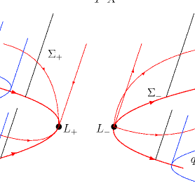
Figure 2. The components $\Sigma_{\hbar,\pm}$ of the semiclassical characteristic set in $\overline{T}^{*}X$, which are now two-dimensional in the figure. The cosphere bundle is the horizontal plane at the bottom of the picture; the intersection of this figure with the cosphere bundle is what is shown on Figure 1. The submanifolds $L_{\pm}$ are still points, with $L_{-}$ a source, $L_{+}$ a sink. The red lines are bicharacteristics, with the thick ones inside $S^{*}X=\partial\overline{T}^{*}X$. The blue regions near the edges show the absorbing region, i.e. the support of $q$. For $P_{h,z}-\imath Q_{h,z}$, the estimates are always propagated away from $L_{\pm}$ towards the support of $q$, so in the direction of the Hamilton flow in $\Sigma_{\hbar,-}$, and in the direction opposite of the Hamilton flow in $\Sigma_{\hbar,+}$; for $P_{h,z}^{*}+\imath Q_{h,z}^{*}$, the directions are reversed.

Microlocal results analogous to the classical results also exist in the semiclassical setting. In the interior of $\overline{T}^{*}X$, i.e. in $T^{*}X$, only the microlocal elliptic, real principal type and complex absorption estimates are relevant. At $L_{\pm}\subset S^{*}X$ we in addition need the analogue of Propositions 2.2-2.3. As these are the only non-standard estimates, though they are very similar to estimates of [56], where, however, only global estimates were stated, we explicitly state these here and indicate the very minor changes needed in the proof compared to Propositions 2.2-2.3.

Proposition 2.9.

For all $N$, for $s\geq m>(k-1-\beta\operatorname{Im}\sigma)/2$, $\sigma=h^{-1}z$, and for all $A,B,G\in\Psi_{\hbar}^{0}(X)$ such that $\mathrm{WF}_{h}^{\prime}(G)\cap\mathrm{WF}_{h}^{\prime}(Q_{\sigma})=\emptyset$, $A$ elliptic at $L_{\pm}$, and forward (or backward) bicharacteristics from $\mathrm{WF}_{h}^{\prime}(B)$ tend to $L_{\pm}$, with closure in the elliptic set of $G$, one has estimates

(2.23) $$Au\in H^{m}_{h}\Rightarrow\|Bu\|_{H^{s}_{h}}\leq C(h^{-1}\|GP_{h,z}u\|_{H^{s-k+1}_{h}}+h\|u\|_{H^{-N}_{h}}),$$

where, as usual, $GP_{h,z}u\in H^{s-k+1}_{h}$ and $u\in H^{-N}_{h}$ are assumptions implied by the right hand side.

Proposition 2.10.

For $s<(k-1-\beta\operatorname{Im}\sigma)/2$, for all $N$, $\sigma=h^{-1}z$, and for all $A,B,G\in\Psi_{\hbar}^{0}(X)$ such that $\mathrm{WF}_{h}^{\prime}(G)\cap\mathrm{WF}_{h}^{\prime}(Q_{\sigma})=\emptyset$, $B,G$ elliptic at $L_{\pm}$, and forward (or backward) bicharacteristics from $\mathrm{WF}_{h}^{\prime}(B)\setminus L_{\pm}$ reach $\mathrm{WF}_{h}^{\prime}(A)$, while remaining in the elliptic set of $G$, one has estimates

(2.24) $$\|Bu\|_{H^{s}_{h}}\leq C(h^{-1}\|GP_{h,z}^{*}u\|_{H^{s-k+1}_{h}}+\|Au\|_{H^{s}_{h}}+h\|u\|_{H^{-N}_{h}}).$$

Proof.

We just need to localize in $\tilde{\rho}$ in addition to $\rho_{0}$; such a localization in the classical setting is implied by working on $S^{*}X$ or with homogeneous symbols. We achieve this by modifying the localizer $\phi$ in the commutant constructed in the proof of Propositions 2.2-2.3. As already remarked, the proof is much like at radial points in semiclassical scattering on asymptotically Euclidean spaces, studied by Vasy and Zworski [56], but we need to be more careful about localization in $\rho_{0}$ and $\tilde{\rho}$ as we are assuming less about the structure.

First, note that $L_{\pm}$ is defined by $\tilde{\rho}=0$, $\rho_{0}=0$, so $\tilde{\rho}^{2}+\rho_{0}$ is a quadratic defining function of $L_{\pm}$. Thus, let $\phi\in\mathcal{C}^{\infty}_{c}(\mathbb{R})$ be identically $1$ near $0$, $\phi^{\prime}\leq 0$ and $\phi$ supported sufficiently close to $0$ so that

$$\begin{split}&\tilde{\rho}^{2}+\rho_{0}\in\operatorname{supp}d\phi\Rightarrow\mp\tilde{\rho}^{k-1}(\mathsf{H}_{p}\rho_{0}+2\tilde{\rho}\mathsf{H}_{p}\tilde{\rho})>0\end{split}$$

and

$$\begin{split}&\tilde{\rho}^{2}+\rho_{0}\in\operatorname{supp}\phi\Rightarrow\mp\tilde{\rho}^{k-2}\mathsf{H}_{p}\tilde{\rho}>0.\end{split}$$

Such $\phi$ exists by (2.3) and (2.4) as

$$\mp\tilde{\rho}(\mathsf{H}_{p}\rho_{0}+2\tilde{\rho}\mathsf{H}_{p}\tilde{\rho})\geq\beta_{1}\rho_{0}+2\beta_{0}\tilde{\rho}^{2}-\mathcal{O}((\tilde{\rho}^{2}+\rho_{0})^{3/2}).$$

Then let $c$ be given by

$$c=\phi(\rho_{0}+\tilde{\rho}^{2})\tilde{\rho}^{-s+(k-1)/2},\qquad c_{\epsilon}=c(1+\epsilon\tilde{\rho}^{-1})^{-\delta}.$$

The rest of the proof proceeds exactly as for Propositions 2.2-2.3. ∎

We first show that under extra assumptions, giving semiclassical ellipticity for $\operatorname{Im}z$ bounded away from $0$, we have non-trapping estimates. So assume that for $|\operatorname{Im}z|>\epsilon>0$, $p_{\hbar,z}$ is semiclassically elliptic on $T^{*}X$ (but not necessarily at $S^{*}X=\partial\overline{T}^{*}X$, where the standard principal symbol $p$ already describes the behavior). Also assume that $\pm\operatorname{Im}p_{\hbar,z}\geq 0$ near the classical characteristic set $\Sigma_{\hbar,\pm}\subset S^{*}X$. Assume also that $p_{\hbar,z}-\imath q_{\hbar,z}$ is elliptic for $|\operatorname{Im}z|>\epsilon>0$, $h^{-1}z\in\Omega$, and $\mp\operatorname{Re}q_{\hbar,z}\geq 0$ near the classical characteristic set $\Sigma_{\hbar,\pm}\subset S^{*}X$. Then the semiclassical version of the classical results (with ellipticity in $T^{*}X$ making these trivial except at $S^{*}X$) apply. Let $H^{s}_{h}$ denote the usual semiclassical function spaces. Then, on the one hand, for any $s\geq m>(k-1-\beta\operatorname{Im}z/h)/2$, $h<h_{0}$,

(2.25) $$\|u\|_{H^{s}_{h}}\leq Ch^{-1}(\|(P_{h,z}-\imath Q_{h,z})u\|_{H^{s-k+1}_{h}}+h^{2}\|u\|_{H^{m}_{h}}),$$

and on the other hand, for any $N$ and for any $s<(k-1+\beta\operatorname{Im}z/h)/2$, $h<h_{0}$,

(2.26) $$\|u\|_{H^{s}_{h}}\leq Ch^{-1}(\|(P_{h,z}^{*}+\imath Q_{h,z}^{*})u\|_{H^{s-k+1}_{h}}+h^{2}\|u\|_{H^{-N}_{h}}).$$

The $h^{2}$ term can be absorbed in the left hand side for sufficiently small $h$, so we automatically obtain invertibility of $P_{h,z}-\imath Q_{h,z}$.

In particular, $P_{h,z}-\imath Q_{h,z}$ is invertible for $h^{-1}z\in\Omega$ with $\operatorname{Im}z>\epsilon>0$ and $h$ small, i.e. $P_{\sigma}-\imath Q_{\sigma}$ is such for $\sigma\in\Omega$ in a cone bounded away from the real axis with $\operatorname{Im}\sigma$ sufficiently large, proving the meromorphy of $P_{\sigma}-\imath Q_{\sigma}$ under these extra assumptions. Note also that for instance

$$\|u\|^{2}_{H_{|\sigma|^{-1}}^{1}}=\|u\|_{L^{2}}^{2}+|\sigma|^{-2}\|du\|_{L^{2}}^{2},\qquad\|u\|_{H_{|\sigma|^{-1}}^{0}}=\|u\|_{L^{2}},$$

(with the norms with respect to any positive definite inner product).

Theorem 2.11.

Let $P_{\sigma}$, $Q_{\sigma}$, $\beta$, $\mathbb{C}_{s}$ be as above, and $\mathcal{X}^{s}$, $\mathcal{Y}^{s}$ as in (2.20). Then, for $\sigma\in\mathbb{C}_{s}\cap\Omega$,

$$P_{\sigma}-\imath Q_{\sigma}:\mathcal{X}^{s}\to\mathcal{Y}^{s}$$

has a meromorphic inverse

$$R(\sigma):\mathcal{Y}^{s}\to\mathcal{X}^{s}.$$

Moreover, for all $\epsilon>0$ there is $C>0$ such that it is invertible in $\operatorname{Im}\sigma>C+\epsilon|\operatorname{Re}\sigma|$, $\sigma\in\Omega$, and non-trapping estimates hold:

$$\|R(\sigma)f\|_{H^{s}_{|\sigma|^{-1}}}\leq C^{\prime}|\sigma|^{-k+1}\|f\|_{H^{s-1}_{|\sigma|^{-1}}}.$$

Remark 2.12.

In fact, the large $\operatorname{Im}\sigma$ behavior of $P_{\sigma}-\imath Q_{\sigma}$ does not matter for our main results, except the support conclusion of the existence part of Lemma 3.1, and the analogous statement in its consequences, Proposition 3.5 and Corollary 3.10. In particular, when the solution is known to exist in a weighted b-Sobolev space, the large $\operatorname{Im}\sigma$ behavior is not used at all; for existence the only loss would be that the solution would not have the stated support property (which is desirable to have in the wave equation setting). The behavior when $\operatorname{Im}\sigma$ is bounded, but $\operatorname{Re}\sigma$ goes to infinity, which we now discuss, is, on the other hand, more crucial, and depends on the more delicate Hamiltonian dynamics (but not on the ellipticity for non-real $z$ which we just discussed).

To deal with estimates for $z$ (almost) real, we need additional assumptions. We make the non-trapping assumption into a definition:

Definition 2.13.

We say that $p_{\hbar,z}-\imath q_{\hbar,z}$ is semiclassically non-trapping if the bicharacteristics from any point in $\Sigma_{\hbar}\setminus(L_{+}\cup L_{-})$ flow to $\mathrm{ell}(q_{\hbar,z})\cup L_{+}$ (i.e. either enter $\mathrm{ell}(q_{\hbar,z})$ at some finite time, or tend to $L_{+}$) in the forward direction, and to $\mathrm{ell}(q_{\hbar,z})\cup L_{-}$ in the backward direction.

Remark 2.14.

The part of the semiclassically non-trapping property on $S^{*}X$ is just the classical non-trapping property; thus, the point is its extension into to the interior $T^{*}X$ of $\overline{T}^{*}X$. Since the classical principal symbol is assumed real, there did not need to be any additional restrictions on $\operatorname{Im}p_{\hbar,z}$ there.

The semiclassical version of all of the above estimates are then applicable for $\operatorname{Im}z\geq-Ch$, and one obtains on the one hand that for any $s\geq m>(k-1-\beta\operatorname{Im}z/h)/2$, $h<h_{0}$,

(2.27) $$\|u\|_{H^{s}_{h}}\leq Ch^{-1}(\|(P_{h,z}-\imath Q_{h,z})u\|_{H^{s-k+1}_{h}}+h^{2}\|u\|_{H^{m}_{h}}),$$

On the other hand, for any $N$ and for any $s<(k-1+\beta\operatorname{Im}z/h)/2$, $h<h_{0}$,

(2.28) $$\|u\|_{H^{s}_{h}}\leq Ch^{-1}(\|(P_{h,z}^{*}+\imath Q_{h,z}^{*})u\|_{H^{s-k+1}_{h}}+h^{2}\|u\|_{H^{-N}_{h}}),$$

The $h^{2}$ term can again be absorbed in the left hand side for sufficiently small $h$, so we automatically obtain invertibility of $P_{h,z}-\imath Q_{h,z}$.

Translated into the classical setting this gives

Theorem 2.15.

Let $P_{\sigma}$, $Q_{\sigma}$, $\mathbb{C}_{s}$, $\beta$ be as above, in particular semiclassically non-trapping, and $\mathcal{X}^{s}$, $\mathcal{Y}^{s}$ as in (2.20). Let $C>0$. Then there exists $\sigma_{0}$ such that

$$R(\sigma):\mathcal{Y}^{s}\to\mathcal{X}^{s},$$

is holomorphic in $\{\sigma\in\Omega:\ \operatorname{Im}\sigma>-C,\ |\operatorname{Re}\sigma|>\sigma_{0}\}$, assumed to be a subset of $\mathbb{C}_{s}$, and non-trapping estimates

$$\|R(\sigma)f\|_{H^{s}_{|\sigma|^{-1}}}\leq C^{\prime}|\sigma|^{-k+1}\|f\|_{H^{s-k+1}_{|\sigma|^{-1}}}$$

hold. For $s=1$, $k=2$ this states that for $|\operatorname{Re}\sigma|>\sigma_{0}$, $\operatorname{Im}\sigma>-C$,

$$\|R(\sigma)f\|_{L^{2}}^{2}+|\sigma|^{-2}\|dR(\sigma)\|_{L^{2}}^{2}\leq C^{\prime\prime}|\sigma|^{-2}\|f\|_{L^{2}}^{2}.$$

Analogous results work for other Sobolev spaces; $H^{1}_{h}$ was chosen above for simplicity.

Remark 2.16.

We emphasize that if semiclassical non-trapping assumptions are made, but not ellipticity for $z$ non-real, meromorphy still follows by taking $h$ small and $z>0$, say, to get a point of invertibility. This is useful because one can eliminate the need to conjugate by a factor to induce such ellipticity when the resulting estimate is irrelevant. (Mostly estimates in strips for $h^{-1}z$, i.e. $\mathcal{O}(h)$ estimates for $z$, matter.) However, there is a cost: while only finitely many poles can lie in any strip $|\operatorname{Im}\sigma|<C$, there is no need for this statement to hold if we allow $\operatorname{Im}\sigma>-C$. Since, for the application to the wave equation, $\operatorname{Im}\sigma$ depends on the a priori growth rate of the solution $u$ which we are Mellin transforming, this would mean that depending on the a priori growth rate one could get more (faster growing) terms in the expansion of $u$ if one relaxes the growth condition on $u$.

While we stated just the global results here, of course one has microlocal estimates for the solution. In particular we have the following, stated in the semiclassical language, as immediate from the estimates used to derive from the Fredholm property:

Theorem 2.17.

Let $P_{\sigma}$, $Q_{\sigma}$, $\beta$ be as above, in particular semiclassically non-trapping, and $\mathcal{X}^{s}$, $\mathcal{Y}^{s}$ as in (2.20).

For $\operatorname{Re}z>0$ and $s^{\prime}>s$, the resolvent $R_{h,z}$ is semiclassically outgoing with a loss of $h^{-1}$ in the sense that if $\alpha\in\overline{T}^{*}X\cap\Sigma_{\hbar,\pm}$, and if for the forward ($+$), resp. backward ($-$), bicharacteristic $\gamma_{\pm}$, from $\alpha$, $\mathrm{WF}_{h}^{s^{\prime}-k+1}(f)\cap\overline{\gamma_{\pm}}=\emptyset$ then $\alpha\notin\mathrm{WF}_{h}^{s^{\prime}}(hR_{h,z}f)$.

In fact, for any $s^{\prime}\in\mathbb{R}$, the resolvent $R_{h,z}$ extends to $f\in H^{s^{\prime}}_{h}(X)$, with non-trapping bounds, provided that $\mathrm{WF}_{h}^{s}(f)\cap(L_{+}\cup L_{-})=\emptyset$. The semiclassically outgoing with a loss of $h^{-1}$ result holds for such $f$ and $s^{\prime}$ as well.

Proof.

The only part that is not immediate by what has been discussed is the last claim. This follows immediately, however, by microlocal solvability in arbitrary ordered Sobolev spaces away from the radial points (i.e. solvability modulo $\mathcal{C}^{\infty}$, with semiclassical estimates), combined with our preceding results to deal with this smooth remainder plus the contribution near $L_{+}\cup L_{-}$, which are assumed to be in $H^{s}_{h}(X)$. ∎

This result is needed for gluing constructions as in [15], namely polynomially bounded trapping with appropriate microlocal geometry can be glued to our resolvent. Furthermore, it gives non-trapping estimates microlocally away from the trapped set provided the overall (trapped) resolvent is polynomially bounded as shown by Datchev and Vasy [16].

Definition 2.18.

Suppose $K_{\pm}\subset T^{*}X$ is compact, and $O_{\pm}$ is a neighborhood of $K$ with compact closure and $O_{\pm}\cap\Sigma_{\hbar}\subset\Sigma_{\hbar,\pm}$. We say that $p_{\hbar,z}$ is semiclassically locally mildly trapping of order $\varkappa$ in a $C_{0}$-strip if

1. there is a function $F\in\mathcal{C}^{\infty}(T^{*}X)$, $F\geq 2$ on $K_{\pm}$, $F\leq 1$ on $T^{*}X\setminus O_{\pm}$, and for $\alpha\in(O_{\pm}\setminus K_{\pm})\cap\Sigma_{\hbar,\pm}$, $(\mathsf{H}_{p_{\hbar,z}}F)(\alpha)=0$ implies $(\mathsf{H}_{p_{\hbar,z}}^{2}F)(\alpha)<0$; and

2. there exists $\tilde{Q}_{h,z}\in\Psi_{\hbar}(X)$ with $\mathrm{WF}_{h}^{\prime}(\tilde{Q}_{h,z})\cap K_{\pm}=\emptyset$, $\mp\tilde{q}_{\hbar,z}\geq 0$ near $\Sigma_{\hbar,\pm}$, $\tilde{q}_{\hbar,z}$ elliptic on $\Sigma_{\hbar}\setminus(O_{+}\cup O_{-})$ and $h_{0}>0$ such that if $\operatorname{Im}z>-C_{0}h$ and $h<h_{0}$ then

   (2.29) $$\|(P_{h,z}-\imath\tilde{Q}_{h,z})^{-1}f\|_{H^{s}_{h}}\leq Ch^{-\varkappa-1}\|f\|_{H^{s-k+1}_{h}},\ f\in H^{s-k+1}_{h}.$$

We say that $p_{\hbar,z}-\imath q_{\hbar,z}$ is semiclassically mildly trapping of order $\varkappa$ in a $C_{0}$-strip if it is semiclassically locally mildly trapping of order $\varkappa$ in a $C_{0}$-strip and if the bicharacteristics from any point in $\Sigma_{\hbar,+}\setminus(L_{+}\cup K_{+})$ flow to $\{q_{\hbar,z}<0\}\cup O_{+}$ in the backward direction and to $\{q_{\hbar,z}<0\}\cup O_{+}\cup L_{+}$ in the forward direction, while the bicharacteristics from any point in $\Sigma_{\hbar,-}\setminus(L_{-}\cup K_{-})$ flow to $\{q_{\hbar,z}>0\}\cup O_{-}\cup L_{-}$ in the backward direction and to $\{q_{\hbar,z}>0\}\cup O_{-}$ in the forward direction.

An example of locally mild trapping is hyperbolic trapping, studied by Wunsch and Zworski [60], which is of order $\varkappa$ for some $\varkappa>0$. Note that (i) states that the sets $K_{c}=\{F\geq c\}$, $1<c<2$, are bicharacteristically convex in $O_{\pm}$, for by (i) any critical points of $F$ along a bicharacteristic are strict local maxima.

As a corollary, we have:

Theorem 2.19.

Let $P_{\sigma}$, $Q_{\sigma}$, $\mathbb{C}_{s}$, $\beta$ be as above, satisfying mild trapping assumptions with order $\varkappa$ estimates in a $C_{0}$-strip, and $\mathcal{X}^{s}$, $\mathcal{Y}^{s}$ as in (2.20). Then there exists $\sigma_{0}$ such that

$$R(\sigma):\mathcal{Y}^{s}\to\mathcal{X}^{s},$$

is holomorphic in $\{\sigma\in\Omega:\operatorname{Im}\sigma>-C_{0},\ |\operatorname{Re}\sigma|>\sigma_{0}\}$, assumed to be a subset of $\mathbb{C}_{s}$, and

(2.30) $$\|R(\sigma)f\|_{H^{s}_{|\sigma|^{-1}}}\leq C^{\prime}|\sigma|^{\varkappa-k+1}\|f\|_{H^{s-k+1}_{|\sigma|^{-1}}}.$$

Further, if one has logarithmic loss in (2.29), i.e. if $h^{-\varkappa}$ can be replaced by $\log(h^{-1})$, for $\sigma\in\mathbb{R}$, (2.30) also holds with a logarithmic loss, i.e. $|\sigma|^{\varkappa}$ can be replaced by $\log|\sigma|$ for $\sigma$ real.

Proof.

This is an almost immediate consequence of [15]. To get into that setting, we replace $Q_{h,z}$ by $Q^{\prime}_{h,z}$ with $\mathrm{WF}_{h}^{\prime}(Q_{h,z}-Q^{\prime}_{h,z})\subset O_{+}\cup O_{-}$ and $Q^{\prime}_{h,z}$ elliptic on $K_{+}\cup K_{-}$, with $\mp q^{\prime}_{\hbar,z}\geq 0$ on $\Sigma_{\hbar,\pm}$. Then $P_{h,z}-\imath Q^{\prime}_{h,z}$ is semiclassically non-trapping in the sense discussed earlier, so all of our estimates apply. With the polynomial resolvent bound assumption on $P_{h,z}-\imath\tilde{Q}_{h,z}$, and the function $F$ in place of $x$ used in [15], the results of [15] apply, taking into account Theorem 2.17 and [15, Lemma 5.1]. Note that the results of [15] are stated in a slightly different context for convenience, namely the function $x$ is defined on the manifold $X$ and not on $T^{*}X$, but this is a minor issue: the results and proofs apply verbatim in our setting. ∎

3. Mellin transform and Lorentzian b-metrics

3.1. The Mellin transform

In this section we discuss the basics of Melrose’s b-analysis on an $n$-dimensional manifold with boundary $\bar{M}$, where the boundary is denoted by $X$. We refer to [43] as a general reference. In the main cases of interest here, the b-geometry is trivial, and $\bar{M}=X\times[0,\infty)_{\tau}$ with respect to some (almost) canonical (to the problem) product decomposition. Thus, the reader should feel comfortable in trivializing all the statements below with respect to this decomposition. In this trivial case, the main result on the Mellin transform, Lemma 3.1 is fairly standard, with possibly different notation of the function spaces; we include it here for completeness.

First, recall that the Lie algebra of b-vector fields, $\mathcal{V}_{\mathrm{b}}(\bar{M})$ consists of $\mathcal{C}^{\infty}$ vector fields on $\bar{M}$ tangent to the boundary. In local coordinates $(\tau,y)$, such that $\tau$ is a boundary defining function, they are of the form $a_{n}\tau\partial_{\tau}+\sum_{j=1}^{n-1}a_{j}\partial_{y_{j}}$, with $a_{j}$ arbitrary $\mathcal{C}^{\infty}$ functions. Correspondingly, they are the set of all smooth sections of a $\mathcal{C}^{\infty}$ vector bundle, ${}^{{\mathrm{b}}}T\bar{M}$, with local basis $\tau\partial_{\tau},\partial_{y_{1}},\ldots,\partial_{y_{n-1}}$. The dual bundle, ${}^{{\mathrm{b}}}T^{*}\bar{M}$, thus has a local basis given by $\frac{d\tau}{\tau},dy_{1},\ldots,dy_{n-1}$. All tensorial constructions, such as form and density bundles, go through as usual.

The natural bundles related to the boundary are reversed in the b-setting. Thus, the b-normal bundle of the boundary $X$ is well-defined as the span of $\tau\partial_{\tau}$ defined using any coordinates, or better yet, as the kernel of the natural map $\iota:{}^{{\mathrm{b}}}T_{m}\bar{M}\to T_{m}\bar{M}$, $m\in X$, induced via the inclusion $\mathcal{V}_{\mathrm{b}}(\bar{M})\to\mathcal{V}(\bar{M})$, so

$$a_{n}\tau\partial_{\tau}+\sum_{j=1}^{n-1}a_{j}\partial_{y_{j}}\mapsto\sum_{j=1}^{n-1}a_{j}\partial_{y_{j}},\qquad a_{j}\in\mathbb{R}.$$

Its annihilator in ${}^{{\mathrm{b}}}T^{*}_{m}\bar{M}$ is called the b-cotangent bundle of the boundary; in local coordinates $(\tau,y)$ it is spanned by $dy_{1},\ldots,dy_{n-1}$. Invariantly, it is the image of $T^{*}_{m}\bar{M}$ in ${}^{{\mathrm{b}}}T^{*}_{m}\bar{M}$ under the adjoint of the tangent bundle map $\iota$; as this has kernel $N^{*}_{m}X$, ${}^{{\mathrm{b}}}T^{*}_{m}\bar{M}$ is naturally identified with $T^{*}_{m}X=T^{*}_{m}\bar{M}/N^{*}_{m}X$.

The algebra of differential operators generated by $\mathcal{V}_{\mathrm{b}}(\bar{M})$ over $\mathcal{C}^{\infty}(\bar{M})$ is denoted $\mathrm{Diff}_{\mathrm{b}}(\bar{M})$; in local coordinates as above, elements of $\mathrm{Diff}_{\mathrm{b}}^{k}(\bar{M})$ are of the form

$$\mathcal{P}=\sum_{j+|\alpha|\leq k}a_{j\alpha}(\tau D_{\tau})^{j}D_{y}^{\alpha}$$

in the usual multiindex notation, $\alpha\in\mathbb{N}^{n-1}$, with $a_{j\alpha}\in\mathcal{C}^{\infty}(\bar{M})$. Writing b-covectors as

$$\sigma\,\frac{d\tau}{\tau}+\sum_{j=1}^{n-1}\eta_{j}\,dy_{j},$$

we obtain canonically dual coordinates to $(\tau,y)$, namely $(\tau,y,\sigma,\eta)$ are local coordinates on ${}^{{\mathrm{b}}}T^{*}\bar{M}$. The principal symbol of $\mathcal{P}$ is

(3.1) $$\tilde{p}=\sigma_{{\mathrm{b}},k}(\mathcal{P})=\sum_{j+|\alpha|=k}a_{j\alpha}\sigma^{j}\eta^{\alpha};$$

it is a $\mathcal{C}^{\infty}$ function, which is a homogeneous polynomial of degree $k$ in the fibers, on ${}^{{\mathrm{b}}}T^{*}\bar{M}$. Its Hamilton vector field, $\mathsf{H}_{\tilde{p}}$, is a $\mathcal{C}^{\infty}$ vector field, which is just the extension of the standard Hamilton vector field from $\bar{M}^{\circ}$, is homogeneous of degree $k-1$, on ${}^{{\mathrm{b}}}T^{*}\bar{M}$, and it is tangent to ${}^{{\mathrm{b}}}T^{*}_{X}\bar{M}$. Explicitly, as a change of variables shows, in local coordinates,

(3.2) $$\mathsf{H}_{\tilde{p}}=(\partial_{\sigma}\tilde{p})(\tau\partial_{\tau})+\sum_{j}(\partial_{\eta_{j}}\tilde{p})\partial_{y_{j}}-(\tau\partial_{\tau}\tilde{p})\partial_{\sigma}-\sum_{j}(\partial_{y_{j}}\tilde{p})\partial_{\eta_{j}},$$

so the restriction of $\mathsf{H}_{\tilde{p}}$ to $\tau=0$ is

(3.3) $$\mathsf{H}_{\tilde{p}}|_{{}^{{\mathrm{b}}}T^{*}_{X}\bar{M}}=\sum_{j}(\partial_{\eta_{j}}\tilde{p})\partial_{y_{j}}-\sum_{j}(\partial_{y_{j}}\tilde{p})\partial_{\eta_{j}},$$

and is thus tangent to the fibers (identified with $T^{*}X$) of ${}^{{\mathrm{b}}}T^{*}_{X}M$ over ${}^{{\mathrm{b}}}T^{*}_{X}M/T^{*}X$ (identified with $\mathbb{R}_{\sigma}$).

We next want to define normal operator of $\mathcal{P}\in\mathrm{Diff}_{\mathrm{b}}^{k}(\bar{M})$, obtained by freezing coefficients at $X=\partial\bar{M}$. To do this naturally, we want to extend the ‘frozen operator’ to one invariant under dilations in the fibers of the inward pointing normal bundle ${}_{+}N(X)$ of $X$; see [43, Equation (4.91)]. The latter can always be trivialized by the choice of an inward-pointing vector field $V$, which in turn fixes the differential of a boundary defining function $\tau$ at $X$ by $V\tau|_{X}=1$; given such a choice we can identify ${}_{+}N(X)$ with a product

$$\bar{M}_{\infty}=X\times[0,\infty)_{\tau},$$

with the normal operator being invariant under dilations in $\tau$. Then for $m=(x,\tau)$, ${}^{{\mathrm{b}}}T_{m}\bar{M}_{\infty}$ is identified with ${}^{{\mathrm{b}}}T_{(x,0)}\bar{M}$.

On $\bar{M}_{\infty}$ operators of the form

$$\sum_{j+|\alpha|\leq k}a_{j\alpha}(y)(\tau D_{\tau})^{j}D_{y}^{\alpha},$$

i.e. $a_{j\alpha}\in\mathcal{C}^{\infty}(X)$, are invariant under the $\mathbb{R}^{+}$-action on $[0,\infty)_{\tau}$; its elements are denoted by $\mathrm{Diff}_{{\mathrm{b}},I}(\bar{M}_{\infty})$. The normal operator of $\mathcal{P}\in\mathrm{Diff}_{\mathrm{b}}^{k}(\bar{M})$ is given by freezing the coefficients at $X$:

$$N(\mathcal{P})=\sum_{j+|\alpha|\leq k}a_{j\alpha}(0,y)(\tau D_{\tau})^{j}D_{y}^{\alpha}\in\mathrm{Diff}_{{\mathrm{b}},I}^{k}(\bar{M}_{\infty}).$$

The normal operator family is then defined as

$$\hat{N}(\mathcal{P})(\sigma)=P_{\sigma}=\sum_{j+|\alpha|\leq k}a_{j\alpha}(0,y)\sigma^{j}D_{y}^{\alpha}\in\mathrm{Diff}_{{\mathrm{b}},I}^{k}(\bar{M}_{\infty}).$$

Note also that we can identify a neighborhood of $X$ in $\bar{M}$ with a neighborhood of $X\times\{0\}$ in $\bar{M}_{\infty}$ (this depends on choices), and then transfer $\mathcal{P}$ to an operator (still denoted by $\mathcal{P}$) on $\bar{M}_{\infty}$, extended in an arbitrary smooth manner; then $\mathcal{P}-N(\mathcal{P})\in\tau\mathrm{Diff}_{\mathrm{b}}^{k}(\bar{M}_{\infty})$.

The principal symbol $p$ of the normal operator family, including in the high energy (or, after rescaling, semiclassical) sense, is given by $\sigma_{{\mathrm{b}},k}(\mathcal{P})|_{{}^{{\mathrm{b}}}T^{*}_{X}\bar{M}}$. Correspondingly, the Hamilton vector field, including in the high-energy sense, of $p$ is given by $\mathsf{H}_{\sigma_{{\mathrm{b}},k}(\mathcal{P})}|_{{}^{{\mathrm{b}}}T^{*}_{X}\bar{M}}$; see (3.3). It is useful to note that via this restriction we drop information about $\mathsf{H}_{\sigma_{{\mathrm{b}},k}(\mathcal{P})}$ as a b-vector field, namely the $\tau\partial_{\tau}$ component is neglected. Correspondingly, the dynamics (including at high energies) for the normal operator family is the same at radial points of the Hamilton flow regardless of the behavior of the $\tau\partial_{\tau}$ component, thus whether on ${}^{{\mathrm{b}}}S^{*}\bar{M}=({}^{{\mathrm{b}}}T^{*}\bar{M}\setminus o)/\mathbb{R}^{+}$, with the $\tau$ variable included, we have a source/sink, or a saddle point, with the other (stable/unstable) direction being transversal to the boundary. This is reflected by the same normal operator family showing up in both de Sitter space and in Minkowski space, even though in de Sitter space (and also in Kerr-de Sitter space) in the full b-sense the radial points are saddle points, while in Minkowski space they are sources/sinks (with a neutral direction along the conormal bundle of the event horizon/light cone inside the boundary in both cases).

We now translate our results to solutions of $(\mathcal{P}-\imath\mathcal{Q})u=f$ when $P_{\sigma}-\imath Q_{\sigma}$ is the normal operator family of the b-operator $\mathcal{P}-\imath\mathcal{Q}$. A typical application is when $\mathcal{P}={\square}_{g}$ is the d’Alembertian of a Lorentzian b-metric on $\bar{M}$, discussed in Subsection 3.2.

Thus, consider the Mellin transform in $\tau$, i.e. consider the map

(3.4) $$\mathcal{M}:u\mapsto\hat{u}(\sigma,.)=\int_{0}^{\infty}\tau^{-\imath\sigma}u(\tau,.)\,\frac{d\tau}{\tau},$$

with inverse transform

(3.5) $$\mathcal{M}^{-1}:v\mapsto\check{v}(\tau,.)=\frac{1}{2\pi}\int_{\mathbb{R}+\imath\alpha}\tau^{\imath\sigma}v(\sigma,.)\,d\sigma,$$

with $\alpha$ chosen in the region of holomorphy. Note that for polynomially bounded (in $\tau$) $u$ (with values in a space, such as $\mathcal{C}^{\infty}(X)$, $L^{2}(X)$, $\mathcal{C}^{-\infty}(X)$), for $u$ supported near $\tau=0$, $\mathcal{M}u$ is holomorphic in $\operatorname{Im}\sigma>C$, $C>0$ sufficiently large, with values in the same space (such as $\mathcal{C}^{\infty}(X)$, etc). We discuss more precise statements below. The Mellin transform is described in detail in [43, Section 5], but it is also merely a renormalized Fourier transform, so the results below are simply those for the Fourier transform (often of Paley-Wiener type) after suitable renormalization.

First, Plancherel’s theorem is that if $\nu$ is a smooth non-degenerate density on $X$ and $r_{c}$ denotes restriction to the line $\operatorname{Im}\sigma=c$, then

(3.6) $$r_{-\alpha}\circ\mathcal{M}:\tau^{\alpha}L^{2}(X\times[0,\infty);\frac{|d\tau|}{\tau}\nu)\to L^{2}(\mathbb{R};L^{2}(X;\nu))$$

is an isomorphism. We are interested in functions $u$ supported near $\tau=0$, in which case, with $r_{(c_{1},c_{2})}$ denoting restriction to the strip $c_{1}<\operatorname{Im}\sigma<c_{2}$, for $N>0$,

(3.7) $$\begin{split}&r_{-\alpha,-\alpha+N}\circ\mathcal{M}:\tau^{\alpha}(1+\tau)^{-N}L^{2}(X\times[0,\infty);\frac{|d\tau|}{\tau}\nu)\\ &\qquad\to\Big{\{}v:\mathbb{R}\times\imath(-\alpha,-\alpha+N)\ni\sigma\to v(\sigma)\in L^{2}(X;\nu);\\ &\qquad\qquad v\ \text{is holomorphic in}\ \sigma\ \text{and}\ \sup_{-\alpha<r<-\alpha+N}\|v(.+\imath r,.)\|_{L^{2}(\mathbb{R};L^{2}(X;\nu))}<\infty\Big{\}},\end{split}$$

see [43, Lemma 5.18]. Note that in accordance with (3.6), $v$ in (LABEL:eq:Mellin-range-L2) extends continuously to the boundary values, $r=-\alpha$ and $r=-\alpha-N$, with values in the same space as for holomorphy. Moreover, for functions supported in, say, $\tau<1$, one can take $N$ arbitrary.

Analogous results also hold for the b-Sobolev spaces $H_{{\mathrm{b}}}^{s}(X\times[0,\infty))$. For $s\geq 0$, these can be defined as in [43, Equation (5.41)]:

(3.8) $$\begin{split}&r_{-\alpha}\circ\mathcal{M}:\tau^{\alpha}H_{{\mathrm{b}}}^{s}(X\times[0,\infty);\frac{|d\tau|}{\tau}\nu)\\ &\to\Big{\{}v\in L^{2}(\mathbb{R};H^{s}(X;\nu)):\ v\in(1+|\sigma|^{2})^{s/2}v\in L^{2}(\mathbb{R};L^{2}(X;\nu))\Big{\}},\end{split}$$

with the analogue of (LABEL:eq:Mellin-range-L2) also holding; for $s<0$ one needs to use the appropriate dual statements. See also [43, Equations (5.41)-(5.42)] for differential versions for integer order spaces. Note that the right hand side of (LABEL:eq:b-Sobolev-iso) is equivalent to

(3.9) $$\langle|\sigma|\rangle^{s/2}v\in L^{2}(\mathbb{R};H^{s}_{\langle|\sigma|\rangle^{-1}}(X;\nu)),$$

where the space on the right hand side is the standard semiclassical Sobolev space and $\langle|\sigma|\rangle=(1+|\sigma|^{2})^{1/2}$; indeed, for $s\geq 0$ integer both are equivalent to the statement that for all $\alpha$ with $|\alpha|\leq s$, $\langle|\sigma|\rangle^{s-|\alpha|}D_{y}^{\alpha}v\in L^{2}(\mathbb{R};L^{2}(X;\nu))$. Here by equivalence we mean not only the membership of a set, but also that of the standard norms corresponding to these spaces. Note that by dualization, (3.9) holds for all $s\in\mathbb{R}$.

If $\mathcal{P}-\imath\mathcal{Q}$ is invariant under dilations in $\tau$ on $\bar{M}_{\infty}=X\times[0,\infty)$ then $N(\mathcal{P}-\imath\mathcal{Q})$ can be identified with $\mathcal{P}-\imath\mathcal{Q}$ and we have the following simple lemma:

Lemma 3.1.

Suppose $\mathcal{P}-\imath\mathcal{Q}$ is invariant under dilations in $\tau$ for functions supported near $\tau=0$, and the normal operator family $\hat{N}(\mathcal{P}-\imath\mathcal{Q})$ is of the form $P_{\sigma}-\imath Q_{\sigma}$ satisfying the conditions of Section 2, including semiclassical non-trapping. Let $\sigma_{j}$ be the poles of the meromorphic family $(P_{\sigma}-\imath Q_{\sigma})^{-1}$. Then for $\ell<\beta^{-1}(2s-k+1)$, $\ell\neq-\operatorname{Im}\sigma_{j}$ for any $j$, $(\mathcal{P}-\imath\mathcal{Q})u=f$, $u$ tempered, supported near $\tau=0$, $f\in\tau^{\ell}H_{{\mathrm{b}}}^{s-k+1}(\bar{M}_{\infty})$, $u$ has an asymptotic expansion

(3.10) $$u=\sum_{j}\sum_{\kappa\leq m_{j}}\tau^{\imath\sigma_{j}}(\log|\tau|)^{\kappa}a_{j\kappa}+u^{\prime}$$

with $a_{j\kappa}\in\mathcal{C}^{\infty}(X)$ and $u^{\prime}\in\tau^{\ell}H_{{\mathrm{b}}}^{s}(\bar{M}_{\infty})$.

If instead $N(\mathcal{P}-\imath\mathcal{Q})$ is semiclassically mildly trapping of order $\varkappa$ in a $C_{0}$-strip then for $\ell<C_{0}$ (still with $\ell<\beta^{-1}(2s-k+1)$, $\ell\neq-\operatorname{Im}\sigma_{j}$ for any $j$) and $f\in\tau^{\ell}H_{{\mathrm{b}}}^{s-k+1+\varkappa}(\bar{M}_{\infty})$ one has

(3.11) $$u=\sum_{j}\sum_{\kappa\leq m_{j}}\tau^{\imath\sigma_{j}}(\log|\tau|)^{\kappa}a_{j\kappa}+u^{\prime}$$

with $a_{j\kappa}\in\mathcal{C}^{\infty}(X)$ and $u^{\prime}\in\tau^{\ell}H_{{\mathrm{b}}}^{s}(\bar{M}_{\infty})$.

Conversely, given $f$ in the indicated spaces, with $f$ supported near $\tau=0$, a solution $u$ of $(\mathcal{P}-\imath\mathcal{Q})u=f$ of the form (3.10), resp. (3.11), supported near $\tau=0$ exists.

In either case, the coefficients $a_{j\kappa}$ are given by the Laurent coefficients of $(\mathcal{P}-\imath\mathcal{Q})^{-1}$ at the poles $\sigma_{j}$ applied to $f$, with simple poles corresponding to $m_{j}=0$.

If $f=\sum_{j}\sum_{\kappa\leq m^{\prime}_{j}}\tau^{\alpha_{j}}(\log|\tau|)^{\kappa}b_{j\kappa}+f^{\prime}$, with $f^{\prime}$ in the spaces indicated above for $f$, and $b_{j\kappa}\in H^{s-k+1}(X)$, analogous results hold when the expansion of $f$ is added to the form of (3.10) and (3.11), in the sense of the extended union of index sets, see [43, Section 5.18].

Further, the result is stable under sufficiently small dilation-invariant perturbations in the b-sense, i.e. if $\mathcal{P}^{\prime}$ and $\mathcal{Q}^{\prime}$ are sufficiently close to $\mathcal{P}$ and $\mathcal{Q}$ in $\Psi_{\mathrm{b}}^{k}(\bar{M}_{\infty})$ with $P^{\prime}_{\sigma}$ and $Q^{\prime}_{\sigma}$ possessing real principal symbols, and that of $Q^{\prime}_{\sigma}$ is non-negative, then there is a similar expansion for solutions of $(\mathcal{P}^{\prime}-\imath\mathcal{Q}^{\prime})u=f$.

For $\mathcal{P}^{*}+\imath\mathcal{Q}^{*}$ in place of $\mathcal{P}-\imath\mathcal{Q}$, analogous results apply, but we need $\ell<-\beta^{-1}(2s-k+1)$, and the $a_{j\kappa}$ are not smooth, rather have wave front set in the Lagrangians $\Lambda_{\pm}$.

Remark 3.2.

Thus, for $\mathcal{P}-\imath\mathcal{Q}$, the more terms we wish to obtain in an expansion, the better Sobolev space we need to work in. For $\mathcal{P}^{*}+\imath\mathcal{Q}^{*}$, dually, we need to be in a weaker Sobolev space under the same circumstances. However, these spaces only need to be worse at the radial points, so under better regularity assumptions on $f$ we still get the expansion in better Sobolev spaces away from the radial points — in particular in elliptic regions. This is relevant in our description of Minkowski space.

Remark 3.3.

If the large $\operatorname{Im}\sigma$, i.e. $\operatorname{Im}z\neq 0$, assumptions in Subsection 2.8 are not satisfied (but the assumptions corresponding to a strip, i.e. roughly real $z$, still are), the proof of this lemma still goes through apart from the support conclusion in the existence part. For the existence argument, one can then pick any $\alpha<\ell$ with $(P_{\sigma}-\imath Q_{\sigma})^{-1}$ having no poles on the line $\operatorname{Im}\sigma=-\alpha$; different choices of $\alpha$ result in different solutions. See also Remark 2.12.

Proof.

First consider the expansion. Suppose $\alpha,r\in\mathbb{R}$ are such that $u\in\tau^{\alpha}H_{{\mathrm{b}}}^{r}(\bar{M}_{\infty})$ and $(P_{\sigma}-\imath Q_{\sigma})^{-1}$ has no poles on the line $\operatorname{Im}\sigma=-\alpha$; note that the vanishing of $u$ for $\tau>1$ and the absence of poles of $(P_{\sigma}-\imath Q_{\sigma})^{-1}$ near infinity inside strips (by the semiclassical non-trapping/mildly trapping assumptions) means that this can be arranged, and then also $u\in\tau^{\alpha}(1+\tau)^{-N}H_{{\mathrm{b}}}^{r}(\bar{M}_{\infty})$ for all $N$. The Mellin transform of the PDE, a priori on $\operatorname{Im}\sigma=-\alpha$, is $(P_{\sigma}-\imath Q_{\sigma})\mathcal{M}u=\mathcal{M}f$. Thus,

(3.12) $$\mathcal{M}u=(P_{\sigma}-\imath Q_{\sigma})^{-1}\mathcal{M}f$$

there. If $f\in\tau^{\ell}H_{{\mathrm{b}}}^{s-k+1}(\bar{M}_{\infty})$, then shifting the contour of integration to $\operatorname{Im}\sigma=-\ell$, we obtain contributions from the poles of $(P_{\sigma}-\imath Q_{\sigma})^{-1}$, giving the expansion in (3.10) and (3.11) by Cauchy’s theorem. The error term $u^{\prime}$ is what one obtains by integrating along the new contour in view of the high energy bounds on $(P_{\sigma}-\imath Q_{\sigma})^{-1}$ (which differ as one changes one’s assumption from non-trapping to mild trapping), and the assumptions on $f$.

Conversely, to obtain existence, let $\alpha<\min(\ell,-\sup\operatorname{Im}\sigma_{j})$ and define $u\in\tau^{\alpha}H_{{\mathrm{b}}}^{s}(\bar{M}_{\infty})$ by (3.12) using the inverse Mellin transform with $\operatorname{Im}\sigma=-\alpha$. Then $u$ solves the PDE, hence the expansion follows by the first part of the argument. The support property of $u$ follows from Paley-Wiener, taking into account holomorphy in $\operatorname{Im}\sigma>-\alpha$, and the estimates on $\mathcal{M}f$ and $(P_{\sigma}-\imath Q_{\sigma})^{-1}$ there.

Finally, stability of the expansion follows from Subsection 2.7 since the meromorphy and the large $\sigma$ estimates are stable under such a perturbation. Note that the condition on the principal symbol of $P^{\prime}_{\sigma}$ and $Q^{\prime}_{\sigma}$ to be independent of $\sigma$ is automatically satisfied, for this is just the principal symbol in $\Psi_{\mathrm{b}}^{k}(\bar{M}_{\infty})$ (which stands for one-step, or classical b-pseudodifferential operators) of $\mathcal{P}^{\prime}$ and $\mathcal{Q}^{\prime}$ evaluated at $\sigma=0$ (or any other finite constant), cf. the large parameter discussion at the end of Subsection 2.1. ∎

Remark 3.4.

One actually gets estimates for the coefficients $a_{j\kappa}$ and $u^{\prime}$ in (3.10)-(3.11). Indeed, in view of the isomorphism (3.9) and the contour deformation after (3.12), $u^{\prime}$ is bounded in $\tau^{\ell}H_{{\mathrm{b}}}^{s}(\bar{M}_{\infty})$ by $f$ in $\tau^{\ell}H_{{\mathrm{b}}}^{s-k+1}(\bar{M}_{\infty})$ in the non-trapping case, with the $\varkappa$ shift in the mildly trapping case. Then, in the nontrapping case, the norm of $f$ in $\tau^{\ell}H_{{\mathrm{b}}}^{s-k+1}(\bar{M}_{\infty})$ gives a bound for the norm of $\mathcal{M}f$ on the line $\operatorname{Im}\sigma=-\ell$ in $\langle|\sigma|\rangle^{-(s-k+1)}L^{2}(\mathbb{R};H_{\langle|\sigma|\rangle^{-1}}^{s-k+1}(X))$; now the non-trapping bounds for $(P_{\sigma}-\imath Q_{\sigma})^{-1}$ imply that $(P_{\sigma}-\imath Q_{\sigma})^{-1}\mathcal{M}f$ is bounded in $\langle|\sigma|\rangle^{-s}L^{2}(\mathbb{R};H_{\langle|\sigma|\rangle^{-1}}^{s}(X))$, and thus $u^{\prime}$ is bounded in $\tau^{\ell}H_{{\mathrm{b}}}^{s}(\bar{M}_{\infty})$. One gets similar bounds for the $a_{j\kappa}$; indeed only the norm of $f$ in slightly less weighted spaces (i.e. with a weight $\ell^{\prime}<\ell$) corresponding to the location of the poles of $(P_{\sigma}-\imath Q_{\sigma})^{-1}$ is needed to estimate these. In the case of mild trapping, one needs stronger norms on $f$ corresponding to $\varkappa$ in view of the bounds on $(P_{\sigma}-\imath Q_{\sigma})^{-1}$ then.

One can iterate this to obtain a full expansion even when $\mathcal{P}-\imath\mathcal{Q}$ is not dilation invariant. Note that in most cases considered below, Lemma 3.1 suffices; the exception is if we allow general, non-stationary, b-perturbations of Kerr-de Sitter or Minkowski metrics.

Proposition 3.5.

Suppose $(\mathcal{P}-\imath\mathcal{Q})u=f$, and the normal operator family $\hat{N}(\mathcal{P}-\imath\mathcal{Q})$ is of the form $P_{\sigma}-\imath Q_{\sigma}$ satisfying the conditions of Section 2, including semiclassical non-trapping. Then for $\ell<\beta^{-1}(2(s-|\ell-\alpha|)-k+1)$, $\ell\notin-\operatorname{Im}\sigma_{j}+\mathbb{N}$ for any $j$, $u\in\tau^{\alpha}H_{{\mathrm{b}}}^{r}(\bar{M}_{\infty})$ supported near $0$, $(\mathcal{P}-\imath\mathcal{Q})u=f$, $f\in\tau^{\ell}H_{{\mathrm{b}}}^{s-k+1}(\bar{M}_{\infty})$, $u$ has an asymptotic expansion

(3.13) $$u=\sum_{j}\sum_{l}\sum_{\kappa\leq m_{jl}}\tau^{\imath\sigma_{j}+l}(\log|\tau|)^{\kappa}a_{j\kappa l}+u^{\prime}$$

with $a_{j\kappa}\in\mathcal{C}^{\infty}(X)$ and $u^{\prime}\in\tau^{\ell}H_{{\mathrm{b}}}^{s-[\ell-\alpha]}(\bar{M}_{\infty})$, $[\ell-\alpha]$ being the integer part of $\ell-\alpha$.

If instead $N(\mathcal{P}-\imath\mathcal{Q})$ is semiclassically mildly trapping of order $\varkappa$ in a $C_{0}$-strip then for $\ell<C_{0}$ and $f\in\tau^{\ell}H_{{\mathrm{b}}}^{s-k+1+\varkappa}(\bar{M}_{\infty})$ one has

(3.14) $$u=\sum_{j}\sum_{l}\sum_{\kappa\leq m_{jl}}\tau^{\imath\sigma_{j}+l}(\log|\tau|)^{\kappa}a_{j\kappa l}+u^{\prime}$$

with $a_{j\kappa l}\in\mathcal{C}^{\infty}(X)$ and $u^{\prime}\in\tau^{\ell}H_{{\mathrm{b}}}^{s-[\ell-\alpha]}(\bar{M}_{\infty})$.

If $f=\sum_{j}\sum_{\kappa\leq m^{\prime}_{j}}\tau^{\alpha_{j}}(\log|\tau|)^{\kappa}b_{j\kappa}+f^{\prime}$, with $f^{\prime}$ in the spaces indicated above for $f$, and $b_{j\kappa}\in H^{s-k+1}(X)$, analogous results hold when the expansion of $f$ is added to the form of (3.13) and (3.14) in the sense of the extended union of index sets, see [43, Section 5.18].

If $\sigma_{{\mathrm{b}},k}(\mathcal{P}-\imath\mathcal{Q})$ vanishes on the characteristic set of $N(\mathcal{P}-\imath\mathcal{Q})$ to infinite order in Taylor series at $\tau=0$, then there are no losses in the order of $u^{\prime}$, i.e. one can replace $u^{\prime}\in\tau^{\ell}H_{{\mathrm{b}}}^{s-[\ell-\alpha]}(\bar{M}_{\infty})$ by $u^{\prime}\in\tau^{\ell}H_{{\mathrm{b}}}^{s}(\bar{M}_{\infty})$, and $\ell<\beta^{-1}(2(s-|\ell-\alpha|)-k+1)$ by $\ell<\beta^{-1}(2s-k+1)$, giving the same form as in Lemma 3.1.

Conversely, under the characteristic assumption in the previous paragraph, given $f$ in the indicated spaces, with $f$ supported near $\tau=0$, a solution $u$ of $(\mathcal{P}-\imath\mathcal{Q})u=f+f^{\sharp}$ of the form (3.10), resp. (3.11), $f^{\sharp}\in\tau^{\infty}H_{{\mathrm{b}}}^{s-k+1}(\bar{M}_{\infty})$, resp. $H_{{\mathrm{b}}}^{s-k+1+\varkappa}(\bar{M}_{\infty})$, supported near $\tau=0$, exists.

Again, the result is stable under sufficiently small perturbations, in the b-sense, of $\mathcal{P}$ and $\mathcal{Q}$, in the same sense, apart from dilation invariance, as stated in Lemma 3.1.

Remark 3.6.

The losses in the regularity of $u^{\prime}$ without further assumptions are natural due to the lack of ellipticity. Specifically, if, for instance, $u$ is conormal to a hypersurface $S$ transversal to $X$, as is the case in many interesting examples, the orbits of the $\mathbb{R}^{+}$-action on $\bar{M}_{\infty}$ must be tangent to $S$ to avoid losses of regularity in the Taylor series expansion.

In particular, there are no losses if $(\mathcal{P}-\imath\mathcal{Q})-N(\mathcal{P}-\imath\mathcal{Q})\in\tau\mathrm{Diff}_{\mathrm{b}}^{k-1}(\bar{M}_{\infty})$, rather than merely in $\tau\mathrm{Diff}_{\mathrm{b}}^{k}(\bar{M}_{\infty})$.

We only stated the converse result under the extra characteristic assumption to avoid complications with the Sobolev orders. Global solvability depends on more than the normal operator, which is why we do not state such a result here.

Proof.

One proceeds as in Lemma 3.1, Mellin transforming the problem, but replacing $\mathcal{P}-\imath\mathcal{Q}$ by $N(\mathcal{P}-\imath\mathcal{Q})$. Note that $(\mathcal{P}-\imath\mathcal{Q})-N(\mathcal{P}-\imath\mathcal{Q})\in\tau\mathrm{Diff}_{\mathrm{b}}^{k}(\bar{M}_{\infty})$. We treat

$$\tilde{f}=((\mathcal{P}-\imath\mathcal{Q})-N(\mathcal{P}-\imath\mathcal{Q}))u$$

as part of the right hand side, subtracting it from $f$, so

$$N(\mathcal{P}-\imath\mathcal{Q})u=f-\tilde{f}.$$

If $u\in\tau^{\alpha}H_{{\mathrm{b}}}^{r}(\bar{M}_{\infty})$ is supported near $0$, then $\tilde{f}\in\tau^{\alpha+1}H_{{\mathrm{b}}}^{r}(\bar{M}_{\infty})$, so Lemma 3.1 is applicable with $\ell$ replaced by $\min(\ell,\alpha+1)$. If $\ell\leq\alpha+1$, we are done, otherwise we repeat the argument. Indeed, we now know that $u$ is given by an expansion giving rise to poles of $\mathcal{M}u$ in $\operatorname{Im}\sigma>\alpha+1$ plus an element of $\tau^{\alpha+1}H_{{\mathrm{b}}}^{s}(\bar{M}_{\infty})$, so we also have better information on $\tilde{f}$, namely it is also given by a partial expansion, plus an element of $\tau^{\alpha+2}H_{{\mathrm{b}}}^{s-k}(\bar{M}_{\infty})$, or indeed $\tau^{\alpha+2}H_{{\mathrm{b}}}^{s-k+1}(\bar{M}_{\infty})$ under the characteristic assumption on $\mathcal{P}-\imath\mathcal{Q}$. Using the $f$ with a partial expansion part of Lemma 3.1 to absorb the $\tilde{u}$ terms, we can work with $\ell$ replaced by $\min(\ell,\alpha+2)$. It is this step that starts generating the sum over $l$ in (3.13) and (3.14). The iteration stops in a finite number of steps, completing the proof.

For the existence, define a zeroth approximation $u_{0}$ to $u$ using $N(\mathcal{P}-\imath\mathcal{Q})$ in Lemma 3.1, and iterate away the error $\tilde{f}=((\mathcal{P}-\imath\mathcal{Q})u-N(\mathcal{P}-\imath\mathcal{Q}))u_{0}-f$ in Taylor series. ∎

3.2. Lorentzian metrics

We now review common properties of Lorentzian b-metrics $g$ on $\bar{M}$. Lorentzian b-metrics are symmetric non-degenerate bilinear forms on ${}^{{\mathrm{b}}}T_{m}\bar{M}$, $m\in\bar{M}$, of signature $(1,n-1)$, i.e. the maximal dimension of a subspace on which $g$ is positive definite is exactly 1, which depend smoothly on $m$. In other words, they are symmetric sections of ${}^{{\mathrm{b}}}T^{*}\bar{M}\otimes{}^{{\mathrm{b}}}T^{*}\bar{M}$ which are in addition non-degenerate of Lorentzian signature. Usually it is more convenient to work with the dual metric $G$, which is then a symmetric section of ${}^{{\mathrm{b}}}T\bar{M}\otimes{}^{{\mathrm{b}}}T\bar{M}$ which is in addition non-degenerate of Lorentzian signature.

By non-degeneracy there is a nowhere vanishing b-density associated to the metric, $|dg|$, which in local coordinates $(\tau,y)$ is given by $\sqrt{|\det g|}\frac{|d\tau|}{\tau}\,|dy|$, and which gives rise to a Hermitian (positive definite!) inner product on functions. There is also a non-degenerate, but not positive definite, inner product on the fibers of the b-form bundle, ${}^{{\mathrm{b}}}\Lambda\bar{M}$, and thus, when combined with the aforementioned Hermitian inner product on functions, an inner product on differential forms which is not positive definite only due to the lack of definiteness of the fiber inner product. Thus, $A^{*}$ is defined, as a formal adjoint, for any differential operator $A\in\mathrm{Diff}_{\mathrm{b}}^{k}(\bar{M};{}^{{\mathrm{b}}}\Lambda\bar{M})$ acting on sections of the b-form bundle, such as the exterior derivative, $d$. Thus, $g$ gives rise to the d’Alembertian,

$${\square}_{g}=d^{*}d+dd^{*}\in\mathrm{Diff}_{\mathrm{b}}^{2}(\bar{M};\Lambda\bar{M}),$$

which preserves form degrees. The d’Alembertian on functions is also denoted by ${\square}_{g}$. The principal symbol of ${\square}_{g}$ is

$$\sigma_{{\mathrm{b}},2}({\square}_{g})=G.$$

As discussed above, the normal operator of ${\square}_{g}$ on $\bar{M}$ is $N({\square}_{g})\in\mathrm{Diff}_{{\mathrm{b}},I}(\bar{M}_{\infty})$, $\bar{M}_{\infty}=X\times[0,\infty)_{\tau}$. If $\bar{M}=\bar{M}_{\infty}$ (i.e. it is a product space to start with) and if ${\square}_{g}$ already has this invariance property under a product decomposition, then the normal operator can be identified with ${\square}_{g}$ itself. Taking the Mellin transform in $\tau$, we obtain a family of operators, $P_{\sigma}$, on $X$, depending analytically on $\sigma$, the b-dual variable of $\tau$. The semiclassical principal symbol of $P_{h,z}=h^{2}P_{h^{-1}z}$ is just the dual metric $G$ on the complexified cotangent bundle ${}^{{\mathrm{b}},\mathbb{C}}T^{*}_{m}\bar{M}$, $m=(x,\tau)$, evaluated on covectors $\varpi+z\,\frac{d\tau}{\tau}$, where $\varpi$ is in the (real) span $\Pi$ of the ‘spatial variables’ $T^{*}_{x}X$; thus $\Pi$ and $\frac{d\tau}{\tau}$ are linearly independent. In general,

(3.15) $$\begin{split}&\langle\varpi+z\,\frac{d\tau}{\tau},\varpi+z\,\frac{d\tau}{\tau}\rangle_{G}\\ &=\langle\varpi+\operatorname{Re}z\,\frac{d\tau}{\tau},\varpi+\operatorname{Re}z\,\frac{d\tau}{\tau}\rangle_{G}-(\operatorname{Im}z)^{2}\langle\frac{d\tau}{\tau},\frac{d\tau}{\tau}\rangle_{G}\\ &\qquad+2\imath\operatorname{Im}z\langle\varpi+\operatorname{Re}z\frac{d\tau}{\tau},\frac{d\tau}{\tau}\rangle_{G}.\end{split}$$

For $\operatorname{Im}z\neq 0$, the vanishing of the imaginary part states that $\langle\varpi+\operatorname{Re}z\,\frac{d\tau}{\tau},\frac{d\tau}{\tau}\rangle_{G}=0$; the real part is the first two terms on the right hand side of (LABEL:eq:Lorentz-metric-img).

In the setting of Subsection 2.8 we want that when $\operatorname{Im}z\neq 0$ and $\operatorname{Im}p_{\hbar,z}$ vanishes then $\operatorname{Re}p_{\hbar,z}$ does not vanish, i.e. that on the orthocomplement of the span of $\frac{d\tau}{\tau}$ the metric should have the opposite sign as that of $\langle\frac{d\tau}{\tau},\frac{d\tau}{\tau}\rangle_{G}$. For a Lorentzian metric this is only possible if $\frac{d\tau}{\tau}$ is time-like (note that $\varpi+\operatorname{Re}z\,\frac{d\tau}{\tau}$ spans the whole fiber of the b-cotangent bundle as $\operatorname{Re}z$ and $\varpi\in\Pi$ vary), when, however, this is automatically the case, namely the metric is negative definite on this orthocomplement. From now on we always assume that $\frac{d\tau}{\tau}$ is time-like for $G$.

Furthermore, for $z$ real, non-zero, the characteristic set of $p_{\hbar,z}$ cannot intersect the hypersurface $\langle\varpi+\operatorname{Re}z\frac{d\tau}{\tau},\frac{d\tau}{\tau}\rangle_{G}=0$, for $G$ is negative definite on covectors satisfying this equality, so if the intersection were non-empty, $\varpi+\operatorname{Re}z\frac{d\tau}{\tau}$ would vanish there, which cannot happen for $\varpi\in\Pi$ since $\operatorname{Re}z\neq 0$ by assumption. Correspondingly, we can divide the semiclassical characteristic set in two parts by

(3.16) $$\Sigma_{\hbar,\pm}\cap T^{*}X=\{\varpi\in\Sigma_{\hbar}\cap T^{*}X:\pm\langle\varpi+\operatorname{Re}z\frac{d\tau}{\tau},\frac{d\tau}{\tau}\rangle_{G}>0\};$$

note that by the definiteness of the quadratic form on this hypersurface, in fact this separation holds on the fiber-compactified bundle, $\overline{T}^{*}X$. In general, one of the ‘components’ $\Sigma_{\hbar,\pm}$ may be empty. However, in any case, when $\operatorname{Im}z\geq 0$, the sign of the imaginary part of $p_{\hbar,z}$ on $\Sigma_{\hbar,\pm}$ is given by $\pm\operatorname{Im}p_{\hbar,z}\geq 0$, as needed for the propagation of estimates: in $\Sigma_{\hbar,+}$ we can propagate estimates backwards, in $\Sigma_{\hbar,-}$ we can propagate estimates forward. For $\operatorname{Im}z\leq 0$, the direction of propagation is reversed.

Moreover, for $m\in\bar{M}$, and with $\Pi$ denoting the ‘spatial’ hyperplane in the real cotangent bundle, ${}^{{\mathrm{b}}}T^{*}_{m}\bar{M}$, the Lorentzian nature of $G$ means that for $z$ real and non-zero, the intersection of $\Pi+z\frac{d\tau}{\tau}$ with the zero-set of $G$ in ${}^{{\mathrm{b}}}T^{*}_{q}\bar{M}$, i.e. the characteristic set, has two components if $G|_{\Pi}$ is Lorentzian, and one component if it is negative definite (i.e. Riemannian, up to the sign). Further, in the second case, on the only component $\langle\varpi+\operatorname{Re}z\frac{d\tau}{\tau},\frac{d\tau}{\tau}\rangle_{G}$ and $\langle\operatorname{Re}z\frac{d\tau}{\tau},\frac{d\tau}{\tau}\rangle_{G}$ have the same sign, so only $\Sigma_{\hbar,\operatorname{sgn}(\operatorname{Re}z)}$ can enter the elliptic region.

We also need information about $p_{\hbar,z}-\imath q_{\hbar,z}$, i.e. when the complex absorption has been added, with $q_{\hbar,z}$ defined for $z$ in an open set $\tilde{\Omega}\subset\mathbb{C}$. Here we need to choose $q_{\hbar,z}$ in such a way as to ensure that $p_{\hbar,z}-\imath q_{\hbar,z}$ does not vanish when $\operatorname{Im}z>0$, but for real $z\neq 0$, $q_{\hbar,z}$ is real and for $z$ sufficiently close to $\mathbb{R}$ with $\operatorname{Im}z\geq 0$, $\mp\operatorname{Re}q_{\hbar,z}\geq 0$ on $\Sigma_{\hbar,\pm}$ (as well as an ellipticity condition that we discuss below (3.17)). In order to arrange this, we take

(3.17) $$\begin{split}q_{\hbar,z}=-\chi f_{z}\langle\varpi+z\frac{d\tau}{\tau},\frac{d\tau}{\tau}\rangle_{G},\qquad&\operatorname{Re}f_{z}\geq 0,\ z\in\mathbb{R}\Rightarrow f_{z}\ \text{is real},\\ &\chi\geq 0,\ \text{independent of}\ z;\end{split}$$

note that if in addition $f_{z}$ is bounded away from $0$ when $z$ is bounded away from $0$ in $\mathbb{R}$, then the above conditions for real $z$ are then automatically satisfied in view of (3.16). In addition, at points where $\chi>0$, $p_{\hbar,z}-\imath q_{\hbar,z}$ does not vanish for $z$ real, since the imaginary part, $q_{\hbar,z}$, is non-zero except when $\langle\varpi+z\frac{d\tau}{\tau},\frac{d\tau}{\tau}\rangle_{G}=0$, but in that case the real part satisfies $p_{\hbar,z}<0$ by (3.16).

Note that $\langle\varpi+z\frac{d\tau}{\tau},\frac{d\tau}{\tau}\rangle_{G}$ rather than the function $\langle\varpi+\operatorname{Re}z\frac{d\tau}{\tau},\frac{d\tau}{\tau}\rangle_{G}$ appearing above is used in the definition of $q_{\hbar,z}$ to make sure that $q_{\hbar,z}$ is holomorphic in $z$ (if $f_{z}$ is such). Thus, if we ensure that for $\operatorname{Im}z>0$,

(3.18) $$\operatorname{Im}\left(\langle\varpi+z\frac{d\tau}{\tau},\frac{d\tau}{\tau}\rangle_{G}^{-1}p_{\hbar,z}\right)>0,$$

then $\operatorname{Im}(\imath f)\geq 0$ shows that $p_{\hbar,z}-\imath q_{\hbar,z}\neq 0$ as desired. We note that the imaginary part of $\langle\varpi+z\frac{d\tau}{\tau},\frac{d\tau}{\tau}\rangle_{G}$ is $\operatorname{Im}z\langle\frac{d\tau}{\tau},\frac{d\tau}{\tau}\rangle_{G}$, and thus is non-zero as $\frac{d\tau}{\tau}$ is time-like and $\operatorname{Im}z>0$. But the expression inside the imaginary part on the left hand side of (3.18) is a positive multiple of $\langle\varpi+\overline{z}\frac{d\tau}{\tau},\frac{d\tau}{\tau}\rangle_{G}p_{\hbar,z}$, so it suffices to consider the latter, whose imaginary part is, with $\beta=\varpi+\operatorname{Re}z\frac{d\tau}{\tau}$,

(3.19) $$\begin{split}&-\operatorname{Im}z\langle\frac{d\tau}{\tau},\frac{d\tau}{\tau}\rangle_{G}\left(\langle\beta,\beta\rangle_{G}-(\operatorname{Im}z)^{2}\langle\frac{d\tau}{\tau},\frac{d\tau}{\tau}\rangle_{G}\right)+\langle\beta,\frac{d\tau}{\tau}\rangle_{G}(2\operatorname{Im}z)\langle\beta,\frac{d\tau}{\tau}\rangle_{G}\\ &=\operatorname{Im}z\left(-\langle\beta,\beta\rangle_{G}\langle\frac{d\tau}{\tau},\frac{d\tau}{\tau}\rangle_{G}+2\langle\beta,\frac{d\tau}{\tau}\rangle_{G}^{2}+(\operatorname{Im}z)^{2}\langle\frac{d\tau}{\tau},\frac{d\tau}{\tau}\rangle_{G}^{2}\right).\end{split}$$

Now, as $\frac{d\tau}{\tau}$ time-like, the first two terms inside the parentheses on the right hand side give twice the positive definite stress-energy tensor; the positive definite character is easily checked by writing $\beta=\gamma+\lambda\frac{d\tau}{\tau}$ with $\langle\gamma,\frac{d\tau}{\tau}\rangle_{G}=0$, for then these terms give

(3.20) $$\langle\frac{d\tau}{\tau},\frac{d\tau}{\tau}\rangle_{G}\left(-\langle\gamma,\gamma\rangle_{G}+\lambda^{2}\langle\frac{d\tau}{\tau},\frac{d\tau}{\tau}\rangle_{G}\right),$$

and the Lorentzian character of $G$ then implies that $-G$ is positive definite on the orthocomplement of the span of $\frac{d\tau}{\tau}$. In view of the third term, $(\operatorname{Im}z)^{2}\langle\frac{d\tau}{\tau},\frac{d\tau}{\tau}\rangle_{G}^{2}$, on the right hand side of (LABEL:eq:p-iq-rotate), we actually conclude that (3.18) holds (i.e. the inequality is strict) when $\operatorname{Im}z>0$.

In fact, typically $p_{\hbar,z}$ itself is not globally defined, so we need to extend it beyond the domain where it is defined. Typically one has a function $\mu$ on $X$ with $d\mu$ time-like for $\mu$ near $\mu_{1}\in\mathbb{R}$, and $p_{\hbar,z}$ is given by a Lorentzian b-metric in $\mu\geq\mu_{1}$, but we need to extend $p_{\hbar,z}$ to $\mu<\mu_{1}$. For this purpose, we first let $\tilde{H}$ to be a Riemannian metric on $X$, and then for some $j\geq 1$ integer we let

$$\hat{p}_{\hbar,z}=\left(\|\varpi\|^{2j}_{\tilde{H}}+z^{2j}\right)^{1/j};$$

thus the case of $j=1$ actually corresponds to a Riemannian b-metric in which $\frac{d\tau}{\tau}$ and $\varpi\in T^{*}_{x}X$ are orthogonal, unlike in the case of $G$. Here we choose the branch of the $j$th root function which is positive along the positive reals and has a branch cut along the negative reals, and take as the domain of $\hat{p}_{\hbar,z}$ the values of $\varpi$ and $z$ for which $\|\varpi\|^{2j}_{\tilde{H}}+z^{2j}$ lies outside the branch cut. Thus, the complement $\mathcal{D}_{j}$ of the rays $z=re^{i\pi(2k+1)/(2j)}$, $k$ an integer, $r\geq 0$, is always in the domain of $\hat{p}_{\hbar,z}$, and thus as $j$ varies, these domains cover any compact set of $\mathbb{C}$ disjoint from $0$. Now let $\mu_{0}>\mu_{0}^{\prime}>\mu_{1}^{\prime}>\mu_{1}$, and choose a partition of unity $\chi_{1}+\chi_{2}=1$, $\chi_{j}\geq 0$, with $\operatorname{supp}\chi_{1}\subset(\mu_{1}^{\prime},+\infty)$, $\operatorname{supp}\chi_{2}\subset(-\infty,\mu_{0}^{\prime})$. Further, with $\digamma>0$ a constant to be chosen, let $\chi\geq 0$ be identically $\digamma$ on $[\mu_{1}^{\prime},\mu_{0}^{\prime}]$ and supported in $(\mu_{1},\mu_{0})$, let

$$f_{z}=\left(\|\varpi\|^{2j}_{\tilde{H}}+z^{2j}\right)^{1/2j},$$

where again the branch cut for the $2j$th root is along the negative reals, so $\hat{p}_{\hbar,z}=f_{z}^{2}$. In particular, note that $\operatorname{Re}f_{z}>0$ with this choice, and even $\operatorname{Re}f_{z}^{2}>0$ if $j\geq 2$. Now, let

(3.21) $$\tilde{p}_{\hbar,z}=\chi_{1}p_{\hbar,z}-\chi_{2}\hat{p}_{\hbar,z},$$

and let $q_{\hbar,z}$ be defined by (3.17). We already know from the above discussion that where $\chi_{1}=1$, $\tilde{p}_{\hbar,z}-\imath q_{\hbar,z}$ satisfies our requirements. We claim that where either $\chi_{2}>0$ or $\chi>0$, $\tilde{p}_{\hbar,z}-\imath q_{\hbar,z}$ is actually elliptic; where $\chi_{2}=0$ but $\chi>0$, this was checked above. Note that as $\|\varpi\|_{\tilde{H}}\to\infty$ and $z$ in a compact set, semiclassical ellipticity becomes a statement (namely, that of ellipticity) for the standard principal symbol, $\tilde{p}-\imath q$, which is easy to check as

$$\tilde{p}-\imath q=\chi_{1}\langle\varpi,\varpi\rangle_{G}-\chi_{2}\|\varpi\|^{2}_{\tilde{H}}-\imath\chi\|\varpi\|_{\tilde{H}}\langle\varpi,\frac{d\tau}{\tau}\rangle,$$

homogeneous of degree $2$ in $\varpi$. Indeed, the imaginary part of $\tilde{p}-\imath q$ only vanishes (for $\varpi\neq 0$) when either $\chi$ or $\langle\varpi,\frac{d\tau}{\tau}\rangle$ does. In the former case, $\chi_{2}=1$ and $\chi_{1}=0$, so $\tilde{p}-\imath q<0$. In the latter case, $\langle\varpi,\varpi\rangle_{G}$ is negative definite, so the real part does not vanish as $\chi_{1}+\chi_{2}=1$. Hence, for sufficiently large $\varpi$, $\tilde{p}_{\hbar,z}-\imath q_{\hbar,z}$ is elliptic in this region; we only need to consider whether it vanishes for finite $\varpi$. Next, if $z$ is real, $z\neq 0$, then $f_{z}>0$,

$$\tilde{p}_{\hbar,z}-\imath q_{\hbar,z}=\chi_{1}\langle\varpi+z\frac{d\tau}{\tau},\varpi+z\frac{d\tau}{\tau}\rangle_{G}-\chi_{2}f_{z}^{2}-\imath\chi f_{z}\langle\varpi+z\frac{d\tau}{\tau},\frac{d\tau}{\tau}\rangle,$$

so again the imaginary part only vanishes if either $\chi$ or $\langle\varpi+z\frac{d\tau}{\tau},\frac{d\tau}{\tau}\rangle$ does. In the former case, $\chi_{2}=1$ and $\chi_{1}=0$ so $\tilde{p}_{\hbar,z}-\imath q_{\hbar,z}<0$. In the latter case, $\langle\varpi+z\frac{d\tau}{\tau},\varpi+z\frac{d\tau}{\tau}\rangle_{G}$ is negative definite, so the real part of $\tilde{p}_{\hbar,z}-\imath q_{\hbar,z}$ is negative. Thus, it remains to consider finite $\varpi$ and non-real $z$, and show that $\tilde{p}_{\hbar,z}-\imath q_{\hbar,z}$ does not vanish then; we have a priori that for $K\subset\mathcal{D}_{j}$ compact (thus disjoint from the branch cuts), there exist $C>0$ and $\delta>0$ such that for $z\in K$ either one of $\|\varpi\|_{\tilde{H}}\geq C$, resp. $|\operatorname{Im}z|\leq\delta$, implies non-vanishing of $\tilde{p}_{\hbar,z}-\imath q_{\hbar,z}$.

To see the remaining cases, i.e. when both $\operatorname{Im}z>\delta$ and $\|\varpi\|_{\tilde{H}}<C$, first assume that $\chi_{2}=1$, so $\chi_{1}=0$. Then

$$\tilde{p}_{\hbar,z}-\imath q_{\hbar,z}=f_{z}\left(-\chi_{2}f_{z}+\imath\chi\langle\varpi+z\frac{d\tau}{\tau},\frac{d\tau}{\tau}\rangle_{G}\right),$$

and the real part of the second factor on the right hand side is

$$-\chi_{2}\operatorname{Re}f_{z}-(\operatorname{Im}z)\chi\langle\frac{d\tau}{\tau},\frac{d\tau}{\tau}\rangle_{G},$$

which is $<0$ as $\chi_{2}>0$ and $\operatorname{Im}z\geq 0$, showing ellipticity.

Now, if neither $\chi_{1}$ nor $\chi_{2}$ vanish, then $\chi>0$. First, suppose that, with $\beta=\varpi+\operatorname{Re}z\frac{d\tau}{\tau}$ as above, $\langle\beta,\frac{d\tau}{\tau}\rangle_{G}=0$, and thus $\langle\beta,\beta\rangle\leq 0$, with the inequality strict if $\beta\neq 0$. Then

$$\tilde{p}_{\hbar,z}-\imath q_{\hbar,z}=\chi_{1}\langle\beta,\beta\rangle_{G}-\chi_{1}(\operatorname{Im}z)^{2}\langle\frac{d\tau}{\tau},\frac{d\tau}{\tau}\rangle_{G}-\chi_{2}f_{z}^{2}-f_{z}\chi(\operatorname{Im}z)\langle\frac{d\tau}{\tau},\frac{d\tau}{\tau}\rangle_{G},$$

so if $\operatorname{Re}f_{z}^{2}>0$, the real part is negative, thus showing ellipticity. On the other hand, if $\langle\beta,\frac{d\tau}{\tau}\rangle_{G}\neq 0$, then we compute

$$\langle\varpi+\overline{z}\frac{d\tau}{\tau},\frac{d\tau}{\tau}\rangle_{G}(\tilde{p}_{\hbar,z}-\imath q_{\hbar,z}).$$

For the $p_{\hbar,z}$ part this is the computation performed in (LABEL:eq:p-iq-rotate) (with an extra factor, $\chi_{1}$, now); on the other hand,

$$\begin{split}\langle\varpi+\overline{z}\frac{d\tau}{\tau},\frac{d\tau}{\tau}\rangle_{G}(-\chi_{2}\hat{p}_{\hbar,z}-\imath q_{\hbar,z})=&-\chi_{2}f_{z}^{2}\left(\langle\beta,\frac{d\tau}{\tau}\rangle_{G}-\imath\operatorname{Im}z\langle\frac{d\tau}{\tau},\frac{d\tau}{\tau}\rangle_{G}\right)\\ &\qquad+\imath\chi f_{z}\left(\langle\beta,\frac{d\tau}{\tau}\rangle_{G}^{2}+(\operatorname{Im}z)^{2}\langle\frac{d\tau}{\tau},\frac{d\tau}{\tau}\rangle_{G}^{2}\right).\end{split}$$

Thus,

$$\begin{split}&\operatorname{Im}\left(\langle\varpi+\overline{z}\frac{d\tau}{\tau},\frac{d\tau}{\tau}\rangle_{G}(-\chi_{2}\hat{p}_{\hbar,z}-\imath q_{\hbar,z})\right)\\ &\qquad=\chi_{2}\operatorname{Re}(f_{z}^{2})\operatorname{Im}z\langle\frac{d\tau}{\tau},\frac{d\tau}{\tau}\rangle_{G}-\chi_{2}\operatorname{Im}(f_{z}^{2})\langle\beta,\frac{d\tau}{\tau}\rangle_{G}\\ &\qquad\qquad+\chi\operatorname{Re}f_{z}\left(\langle\beta,\frac{d\tau}{\tau}\rangle_{G}^{2}+(\operatorname{Im}z)^{2}\langle\frac{d\tau}{\tau},\frac{d\tau}{\tau}\rangle_{G}^{2}\right)\end{split}$$

Combining this with (LABEL:eq:p-iq-rotate) we note that the only term in

$$\begin{split}\operatorname{Im}\Big{(}\langle\varpi+\overline{z}\frac{d\tau}{\tau},\frac{d\tau}{\tau}\rangle_{G}(\tilde{p}_{\hbar,z}-\imath q_{\hbar,z})\Big{)}\end{split}$$

that is not automatically non-negative provided $\operatorname{Im}z\geq 0$, $\operatorname{Re}f_{z}>0$, $\operatorname{Re}(f_{z}^{2})>0$ is $-\chi_{2}\operatorname{Im}(f_{z}^{2})\langle\beta,\frac{d\tau}{\tau}\rangle_{G}$. Thus, if we arrange that

$$2|\chi_{2}|\,|\operatorname{Im}f_{z}|\,|\langle\beta,\frac{d\tau}{\tau}\rangle_{G}|<\frac{\digamma}{2}(\operatorname{Im}z)^{2}\langle\frac{d\tau}{\tau},\frac{d\tau}{\tau}\rangle_{G}^{2},$$

which is guaranteed by choosing $\digamma>0$ sufficiently large as $\operatorname{Im}z>\delta$ and $\beta$ is in a compact set, then in view of the actual positivity of $\chi\operatorname{Re}f_{z}(\operatorname{Im}z)^{2}\langle\frac{d\tau}{\tau},\frac{d\tau}{\tau}\rangle_{G}^{2}$, this imaginary part does not vanish, completing the proof of ellipticity.

In summary, we have shown that if $\frac{d\tau}{\tau}$ is time-like then the assumptions on imaginary part of $p_{\hbar,z}$, as well as on the ellipticity of $p_{\hbar,z}-\imath q_{\hbar,z}$ for non-real $z$, in Section 2 are automatically satisfied in the Lorentzian setting if $q_{\hbar,z}$ is given by (3.17). Further, if we extend $p_{\hbar,z}$ to a new symbol, $\tilde{p}_{\hbar,z}$ across a hypersurface, $\mu=\mu_{1}$, in the manner (3.21), then with $\chi$, $\chi_{1}$ and $\chi_{2}$ as discussed there, $\tilde{p}_{\hbar,z}-\imath q_{\hbar,z}$ satisfies the requirements for $p_{\hbar,z}-\imath q_{\hbar,z}$, and in addition it is elliptic in the extended part of the domain. We usually write $p_{\hbar,z}-\imath q_{\hbar,z}$ for this extension. Thus, these properties need not be checked individually in specific cases.

We remark that $f_{z}$ as above arises from the standard quantization $F_{\sigma}$ of

$$\left(\|\varpi\|^{2j}_{\tilde{H}}+\sigma^{2j}+C^{2j}\right)^{1/2j},$$

for $C>0$ arbitrarily chosen; the large-parameter rescaling $hF_{h^{-1}z}$ of this has the semiclassical principal symbol $f_{z}$. Then for the induced operators $P_{\sigma}-\imath Q_{\sigma}$, the operators are holomorphic in the domain $\Omega_{j,C}$ given with $\mathbb{C}$ with the half-lines $e^{i\pi(2k+1)/(2j)}[C,+\infty)$, $k$ an integer, removed, and thus as $j$ and $C$ vary, these domains cover $\mathbb{C}$.

It is useful to note the following explicit calculation regarding the time-like character of $\frac{d\tau}{\tau}$ if we are given a Lorentzian b-metric $g$ that, with respect to some local boundary defining function ${\tilde{\tau}}$ and local product decomposition $U\times[0,\delta)_{\tilde{\tau}}$ of $\bar{M}$ near $U\subset X$ open, is of the form $G=({\tilde{\tau}}\partial_{{\tilde{\tau}}})^{2}-\tilde{G}$ on $U\times[0,\delta)_{\tilde{\tau}}$, $\tilde{G}$ a Riemannian metric on $U$. In this case, if we define $\tau={\tilde{\tau}}e^{\phi}$, $\phi$ a function on $X$, so $\frac{d\tau}{\tau}=\frac{d{\tilde{\tau}}}{{\tilde{\tau}}}+d\phi$, then

$$\langle\frac{d\tau}{\tau},\frac{d\tau}{\tau}\rangle_{G}=\langle\frac{d{\tilde{\tau}}}{{\tilde{\tau}}},\frac{d{\tilde{\tau}}}{{\tilde{\tau}}}\rangle_{G}-\langle d\phi,d\phi\rangle_{G}=1-\langle d\phi,d\phi\rangle_{\tilde{G}},$$

so $\frac{d\tau}{\tau}$ is time-like if $|d\phi|_{\tilde{G}}<1$. Note that the effect of such a coordinate change on the Mellin transform of the normal operator of ${\square}_{g}$ is conjugation by $e^{-\imath\sigma\phi}$ since ${\tilde{\tau}}^{-\imath\sigma}=\tau^{-\imath\sigma}e^{\imath\sigma\phi}$. Such a coordinate change is useful when $G$ has a product structure on $U\times[0,\delta)_{\tilde{\tau}}$, but ${\tilde{\tau}}$ is only a local boundary defining function on $U\times[0,\delta)_{\tilde{\tau}}$ (the product structure might not extend smoothly beyond $U$), in which case it is useful to see if one can conserve the time-like nature of $\frac{d{\tilde{\tau}}}{{\tilde{\tau}}}$ for a global boundary defining function. This is directly relevant for the study of conformally compact spaces in Subsection 4.9.

Finally, we remark that if $\frac{d\tau}{\tau}$ is time-like and $f$ is supported in $\tau<\tau_{0}$, the forward problem for the wave equation,

$${\square}_{g}u=f,\ u|_{\tau>\tau_{0}}=0,$$

is uniquely solvable on $\bar{M}\setminus X$ near $X$ by standard energy estimates (a priori, without more structure, with no estimates on growth at $X$), see e.g. [32, Chapter 23]. Applying Lemma 3.1 in this case, assuming that the normal operator family has the structure stated there, gives another solution, which must be equal to $u$ by uniqueness. Thus, $u$ has the expansion stated in the lemma.

3.3. Wave equation localization

In this section we recall energy estimates and their consequences when $P_{\sigma}\in\mathrm{Diff}^{2}(X)$ is the wave operator to leading order in a region $\mathcal{O}\subset X$, i.e. when for a Lorentzian metric $h$ on $\mathcal{O}$, $P_{\sigma}-{\square}_{h}\in\mathrm{Diff}^{1}(\mathcal{O})$, and indeed when an analogous statement holds in the ‘large parameter’ sense as well, with the latter naturally arising by Mellin transforming b-wave equations. These results are not needed for the Fredholm properties, but are very useful in describing the asymptotics of the solutions of the wave equation on Kerr-de Sitter space as they show that certain terms arising from cutoffs do not affect the solution. These are also useful for giving an alternative explanation why the choice of the extension of the modified Laplacian across the boundary is unimportant on an (asymptotically) hyperbolic space.

So assume that one is also given a function $t:\mathcal{O}\to(t_{0},t_{1})$ with $dt$ time-like and with $t$ proper on $\mathcal{O}$. Then one has the standard energy estimate; see e.g. [51, Section 2.8] for a version of these estimates (in a slightly different setup):

Proposition 3.7.

Assume $t_{0}<T_{0}<T_{0}^{\prime}<T_{1}$. Then

$$\|u\|_{H^{1}(t^{-1}([T_{0}^{\prime},T_{1}]))}\leq C\left(\|u\|_{H^{1}(t^{-1}([T_{0},T_{0}^{\prime}]))}+\|P_{\sigma}u\|_{L^{2}(t^{-1}([T_{0},T_{1}]))}\right).$$

We also note that in the various estimates in Subsections 2.3-2.5 though the error terms were stated globally as $\|u\|_{H^{-N}}$, in fact they can be localized to any neighborhood $U$ of the projection to the base $X$ of $\mathrm{WF}^{\prime}(G)$.

For us, even more important is a semiclassical version of this estimate. The setup is more conveniently formulated in the large parameter setting, where the large parameter is interpreted as the dual variable of an extra variable of which the operator is independent. So with $\mathcal{O}$ as above, consider the family $P_{\sigma}\in\mathrm{Diff}^{2}(\mathcal{O})$ with large parameter dependence, and assume that the large parameter principal symbol of $P_{\sigma}$, $p_{\sigma}$, is the dual metric function $G$ on $T^{*}\mathcal{O}\times{}^{{\mathrm{b}}}T^{*}\overline{\mathbb{R}^{+}_{\tau}}$ of an $\mathbb{R}^{+}$-invariant (acting as dilations in the second factor on $\mathcal{O}\times\mathbb{R}^{+}$) Lorentzian b-metric $g$, where $\sigma$ is the b-dual variable on ${}^{{\mathrm{b}}}T^{*}\overline{\mathbb{R}^{+}}$. Suppose moreover that, as above, we are also given a function $t:\mathcal{O}\to(t_{0},t_{1})$ with $dt$ time-like and with $t$ proper on $\mathcal{O}$. Then

Proposition 3.8.

Assume $t_{0}<T_{0}<T_{0}^{\prime}<T_{1}<t_{1}$. Then, with $P_{h,z}=h^{2}P_{h^{-1}z}$,

$$\|u\|_{H^{1}_{\hbar}(t^{-1}([T_{0}^{\prime},T_{1}]))}\leq C\left(\|u\|_{H^{1}_{\hbar}(t^{-1}([T_{0},T_{0}^{\prime}]))}+h^{-1}\|P_{h,z}u\|_{L^{2}(t^{-1}([T_{0},T_{1}]))}\right).$$

Proof.

We start by remarking that the $L^{2}$ norm on the right hand side is just the $H^{0}_{\hbar}$ norm, so this is a non-microlocal real principal type estimate except that there is no error term $h\|u\|_{H^{N}_{\hbar}(t^{-1}([T_{0},T_{1}]))}$ norm inside the parentheses on the right hand side (cf. the right hand side of (2.24); although this is stated at a radial point, the estimate has a similar form, without constraints on $s$, away from these), and except that one would usually expect that both $h^{-1}\|P_{h,z}u\|_{L^{2}(t^{-1}([T_{0},T_{1}]))}$ and $h\|u\|_{H^{-N}_{\hbar}(t^{-1}([T_{0},T_{1}]))}$ should in fact be taken on a larger set, such as $t^{-1}([T_{0},T^{\prime}_{1}])$, $T^{\prime}_{1}>T_{1}$. The point is thus to gain these improvements; this is done by a version of the classical energy estimates. We note that of these observations the only truly important part is the absence of a term $h\|u\|_{H^{-N}_{\hbar}(t^{-1}([T_{0},T_{1}^{\prime}]))}$, which is thus on a larger set – this would prevent the argument leading to Proposition 3.9 below.

The following is essentially the standard proof of energy estimates, see e.g. [51, Section 2.8], but in a different context. Here we phrase it as done in [55, Sections 3 and 4]. So consider $V_{\sigma}=-\imath Z_{\sigma}$, $Z_{\sigma}=\chi(t)W_{\sigma}$, and let $W_{\sigma}$ be given by $W=G(dt,.)$ considered as a first order differential operator on $\mathcal{O}$. That is, on $\mathcal{O}\times\mathbb{R}^{+}$, $G(dt,.)$ gives a vector field of the form $W=W^{\prime}+a\,\tau\partial_{\tau}$, with $W^{\prime}$ a vector field on $\mathcal{O}$ and $a$ a function on $\mathcal{O}$ (both independent of $\tau$), and via the Mellin transform one can consider $W$ as $W_{\sigma}=W^{\prime}+a\sigma$, a $\sigma$-dependent first order differential operator on $\mathcal{O}$, with standard large-parameter dependence. Let ${\square}$ be the d’Alembertian of $g$, and let ${\square}_{\sigma}$ be its Mellin conjugate, so $P_{\sigma}-{\square}_{\sigma}$ is first order, even in the large parameter sense, on $\mathcal{O}$. As usual in energy estimates, we want to consider the ‘commutator’

(3.22) $$-\imath(V^{*}_{\sigma}{\square}_{\sigma}-{\square}_{\sigma}V_{\sigma}).$$

While this can easily be computed directly, in order to connect it to the wave equation, we first recall the computation of $-\imath(V^{*}{\square}-{\square}V)$ on $\mathcal{O}\times\mathbb{R}^{+}$, rephrase this in terms of $\mathrm{Diff}_{\mathrm{b}}(\mathcal{O}\times[0,\infty))$; note that ${\square},V\in\mathrm{Diff}_{\mathrm{b}}(\mathcal{O}\times[0,\infty))$ so

$$-\imath(V^{*}{\square}-{\square}V)\in\mathrm{Diff}_{\mathrm{b}}^{2}(\mathcal{O}\times[0,\infty)).$$

Since all operators here are $\mathbb{R}^{+}$-invariant, the b-expressions are mostly a matter of notation. We then Mellin transform to compute (3.22).

Then, the usual computation, see [55, Section 3] for it written down in this form, using the standard summation convention, yields

(3.23) $$\begin{split}&-\imath(V^{*}{\square}-{\square}V)=d^{*}Cd,\ C_{ij}=g_{i\ell}B_{\ell j}\\ &B_{ij}=-J^{-1}\partial_{k}(JZ^{k}G^{ij})+G^{ik}(\partial_{k}Z^{j})+G^{jk}(\partial_{k}Z^{i}),\end{split}$$

where $C_{ij}$ are the matrix entries of $C$ relative to the basis $\{dz_{\ell}\}$ of the fibers of the cotangent bundle (rather than the b-cotangent bundle), $z_{\ell}=y_{\ell}$ for $\ell\leq n-1$, the $y_{\ell}$ local coordinates on a chart in $\mathcal{O}$, $z_{n}=\tau$. Expanding $B$ using $Z=\chi W$, and separating the terms with $\chi$ derivatives, gives

(3.24) $$\begin{split}B_{ij}&=G^{ik}(\partial_{k}Z^{j})+G^{jk}(\partial_{k}Z^{i})-J^{-1}\partial_{k}(JZ^{k}G^{ij})\\ &=(\partial_{k}\chi)\big{(}G^{ik}W^{j}+G^{jk}W^{i}-G^{ij}W^{k}\big{)}\\ &\qquad\qquad\qquad+\chi\big{(}G^{ik}(\partial_{k}W^{j})+G^{jk}(\partial_{k}W^{i})-J^{-1}\partial_{k}(JW^{k}G^{ij})\big{)}.\end{split}$$

Multiplying the first term on the right hand side by $\alpha_{i}\,\overline{\alpha_{j}}$ (and summing over $i,j$; here $\alpha\in\mathbb{C}^{n}\simeq\mathbb{C}T^{*}_{q}(\mathcal{O}\times\mathbb{R}^{+})$, $q\in\mathcal{O}\times\mathbb{R}^{+}$) gives

(3.25) $$\begin{split}E_{W,d\chi}(\alpha)&=(\partial_{k}\chi)(G^{ik}W^{j}+G^{jk}W^{i}-G^{ij}W^{k})\alpha_{i}\,\overline{\alpha_{j}}\\ &=(\alpha,d\chi)_{G}\,\overline{\alpha(W)}+\alpha(W)\,(d\chi,\alpha)_{G}-d\chi(W)(\alpha,\alpha)_{G}=\chi^{\prime}(t)\,E_{W,dt},\\ E_{W,dt}&=(\alpha,dt)_{G}\,\overline{\alpha(W)}+\alpha(W)\,(dt,\alpha)_{G}-dt(W)(\alpha,\alpha)_{G}.\end{split}$$

Now, $E_{W,dt}$ is twice the sesquilinear stress-energy tensor associated to $\alpha$, $W$ and $dt$. This is well-known to be positive definite in $\alpha$, i.e. $E_{W,d\chi}(\alpha)\geq 0$, with vanishing if and only if $\alpha=0$, when $W$ and $dt$ are both forward time-like for smooth Lorentz metrics, see e.g. [51, Section 2.7] or [32, Lemma 24.1.2]; (3.20) provides the computation when $\alpha$ is real.

We change to a local basis of the b-cotangent bundle and use the b-differential ${}^{{\mathrm{b}}}d=(d_{X},\tau\partial_{\tau})$ and the local basis $\{dy_{1},\ldots,dy_{n-1},\frac{d\tau}{\tau}\}$ of the fibers of the b-cotangent bundle, $\hat{\partial}_{j}=\delta_{j}\partial_{j}$, $\delta_{j}=1$ for $j\leq n-1$, $\delta_{n}=\tau$, for the local basis of the fibers of the b-tangent bundle, $\hat{G}^{ij}$, $\hat{g}_{ij}$ the corresponding metric entries, $\hat{Z}^{i}$ the vector field components, yields

(3.26) $$\begin{split}&-\imath(V^{*}{\square}-{\square}V)={}^{{\mathrm{b}}}d^{*}\,\hat{C}\,{}^{{\mathrm{b}}}d,\ \hat{C}_{ij}=\hat{g}_{i\ell}\hat{B}_{\ell j}\\ &\hat{B}_{ij}=-J^{-1}\delta_{k}^{-1}\delta_{i}^{-1}\delta_{j}^{-1}\hat{\partial}_{k}(J\delta_{k}\hat{Z}^{k}\delta_{i}\delta_{j}\hat{G}^{ij})+\hat{G}^{ik}(\delta_{j}^{-1}\hat{\partial}_{k}\delta_{j}\hat{Z}^{j})+\hat{G}^{jk}(\delta_{i}^{-1}\hat{\partial}_{k}\delta_{i}\hat{Z}^{i}).\end{split}$$

While the $\delta$-factors may have non-vanishing derivatives in the above expresson for $\hat{B}$, if these are differentiated, $\chi$ in $\hat{Z}^{i}=\chi\hat{W}^{i}$ is not, so we conclude that

$$\begin{split}\hat{B}_{ij}=&(\hat{\partial}_{k}\chi)\big{(}\hat{G}^{ik}\hat{W}^{j}+\hat{G}^{jk}\hat{W}^{i}-\hat{G}^{ij}\hat{W}^{k}\big{)}\\ &\qquad+\chi\big{(}\hat{G}^{ik}\delta_{j}^{-1}(\hat{\partial}_{k}\delta_{j}W^{j})+G^{jk}\delta_{i}^{-1}(\hat{\partial}_{k}\delta_{i}W^{i})\\ &\qquad\qquad\qquad-J^{-1}\delta_{k}^{-1}\delta_{i}^{-1}\delta_{j}^{-1}\hat{\partial}_{k}(J\delta_{k}\delta_{i}\delta_{j}W^{k}G^{ij})\big{)},\end{split}$$

and so

$$\hat{C}=\chi^{\prime}A+\chi R,$$

with $A$ positive definite.

The Mellin transformed version of (LABEL:eq:b-B_ij-formula) finally computes (3.22); it reads as

$$-\imath(V^{*}_{\sigma}{\square}_{\sigma}-{\square}_{\sigma}V_{\sigma})=d^{*}_{\sigma}\hat{C}d_{\sigma},\ \hat{C}_{ij}=g_{i\ell}B_{\ell j},\ \hat{C}=\chi^{\prime}A+\chi R$$

where $d_{\sigma}=(d_{X},\sigma)$, with the last component being multiplication by $\sigma$, and $A$ is positive definite. Correspondingly,

(3.27) $$\begin{split}-\imath(V^{*}_{\sigma}P_{\sigma}-P_{\sigma}^{*}V_{\sigma})&=-\imath(V^{*}_{\sigma}{\square}_{\sigma}-{\square}_{\sigma}V_{\sigma})-\imath V^{*}_{\sigma}(P_{\sigma}-{\square}_{\sigma})+\imath(P_{\sigma}-{\square}_{\sigma})^{*}V_{\sigma}\\ &=d^{*}_{\sigma}\tilde{C}d_{\sigma}+\hat{E}\chi d_{\sigma}+d_{\sigma}^{*}\chi\hat{E}^{*},\end{split}$$

where $\hat{E}=(\hat{E}_{X},\hat{E}^{\prime})$, $\hat{E}_{X}\in\mathcal{C}^{\infty}(\mathcal{O};TX)$, $\hat{E}^{\prime}\in\mathcal{C}^{\infty}(\mathcal{O})$, and

$$\tilde{C}=\chi^{\prime}A+\chi\tilde{R},$$

since the contribution of $P_{\sigma}-{\square}_{\sigma}$ to second order terms in the large parameter sense is only via terms not differentiated in $\chi$. A standard argument, given below, making $\chi^{\prime}$ large relative to $\chi$, can be used to complete the proof.

Indeed, let $\chi_{0}(s)=e^{-1/s}$ for $s>0$, $\chi_{0}(s)=0$ for $s\leq 0$, $\chi_{1}\in\mathcal{C}^{\infty}(\mathbb{R})$ identically 1 on $[1,\infty)$, vanishing on $(-\infty,0]$, Thus, $s^{2}\chi_{0}^{\prime}(s)=\chi_{0}(s)$ for $s\in\mathbb{R}$. Now let $T_{1}^{\prime}\in(T_{1},t_{1})$, and consider

$$\chi(s)=\chi_{0}(-\digamma^{-1}(s-T^{\prime}_{1}))\chi_{1}((s-T_{0})/(T_{0}^{\prime}-T_{0})),$$

so

$$\operatorname{supp}\chi\subset[T_{0},T^{\prime}_{1}]$$

and

$$s\in[T^{\prime}_{0},T^{\prime}_{1}]\Rightarrow\chi^{\prime}=-\digamma^{-1}\chi_{0}^{\prime}(-\digamma^{-1}(s-T^{\prime}_{1})),$$

so

$$s\in[T^{\prime}_{0},T^{\prime}_{1}]\Rightarrow\chi=-\digamma^{-1}(s-T^{\prime}_{1})^{2}\chi^{\prime},$$

so for $\digamma>0$ sufficiently large, this is bounded by a small multiple of $\chi^{\prime}$, namely

(3.28) $$s\in[T^{\prime}_{0},T^{\prime}_{1}]\Rightarrow\chi\leq-\gamma\chi^{\prime},\ \gamma=(T^{\prime}_{1}-T^{\prime}_{0})^{2}\digamma^{-1}.$$

In particular, for sufficiently large $\digamma$,

$$-(\chi^{\prime}A+\chi R)\geq-\chi^{\prime}A/2$$

on $[T^{\prime}_{0},T^{\prime}_{1}]$. Thus,

$$\langle d^{*}_{\sigma}\tilde{C}d_{\sigma}u,u\rangle\geq-\frac{1}{2}\langle\chi^{\prime}Ad_{\sigma}u,d_{\sigma}u\rangle-C^{\prime}\|d_{\sigma}u\|^{2}_{L^{2}(t^{-1}([T_{0},T^{\prime}_{0}]))}.$$

So for some $c_{0}>0$, by (3.27),

(3.29) $$\begin{split}c_{0}&\|(-\chi^{\prime})^{1/2}d_{\sigma}u\|^{2}\leq-\frac{1}{2}\langle\chi^{\prime}Ad_{\sigma}u,d_{\sigma}u\rangle\\ &\leq C^{\prime}\|d_{\sigma}u\|^{2}_{L^{2}(t^{-1}([T_{0},T^{\prime}_{0}]))}+C^{\prime}\|\chi^{1/2}P_{\sigma}u\|\|\chi^{1/2}d_{\sigma}u\|+C^{\prime}\|\chi^{1/2}u\|\|\chi^{1/2}d_{\sigma}u\|\\ &\leq C^{\prime}\|d_{\sigma}u\|^{2}_{L^{2}(t^{-1}([T_{0},T^{\prime}_{0}]))}+C^{\prime}\|\chi^{1/2}P_{\sigma}u\|^{2}+2C^{\prime}\gamma\|(-\chi^{\prime})^{1/2}d_{\sigma}u\|^{2}\\ &\qquad\qquad\qquad\qquad\qquad\qquad+C^{\prime}\gamma^{-1}|\sigma|^{-1}\|(-\chi^{\prime})^{1/2}d_{\sigma}u\|^{2},\end{split}$$

where we used $\|\chi^{1/2}u\|\leq|\sigma|^{-1}\|\chi^{1/2}d_{\sigma}u\|$ (which holds in view of the last component of $d_{\sigma}$). Thus, choosing first $\digamma>0$ sufficiently large (thus $\gamma>0$ is sufficiently small), and then $|\sigma|$ sufficiently large, the last two terms on the right hand side can be absorbed into the left hand side. Rewriting in the semiclassical notation gives the desired result, except that $\|P_{h,z}u\|_{L^{2}_{\hbar}(t^{-1}([T_{0},T_{1}]))}$ is replaced by $\|P_{h,z}u\|_{L^{2}_{\hbar}(t^{-1}([T_{0},T^{\prime}_{1}]))}$ (or $\|\chi^{1/2}P_{h,z}u\|_{L^{2}_{\hbar}(t^{-1}([T_{0},T^{\prime}_{1}]))}$). This however is easily remedied by replacing $\chi$ by

$$\chi(s)=H(T_{1}-s)\chi_{0}(-\digamma^{-1}(s-T^{\prime}_{1}))\chi_{1}((s-T_{0})/(T_{0}^{\prime}-T_{0})),$$

where $H$ is the Heaviside step function (the characteristic function of $[0,\infty)$) so $\operatorname{supp}\chi\subset[T_{0},T_{1}]$. Now $\chi$ is not smooth, but either approximating $H$ by smooth bump functions and taking a limit, or indeed directly performing the calculation, integtating on the domain with boundary $t\leq T_{1}$, the contribution of the derivative of $H$ to $\chi^{\prime}$ is a delta distribution at $t=T_{1}$, corresponding to a boundary term on the domain, which has the same sign as the derivative of $\chi_{0}$. Thus, with $\mathcal{S}_{T_{1}}$ the hypersurface $\{t=T_{1}\}$, (3.29) holds in the form

$$\begin{split}c_{0}&\|d_{\sigma}u\|^{2}_{L^{2}(t^{-1}([T^{\prime}_{0},T_{1}]))}+c_{0}\|d_{\sigma}u\|^{2}_{L^{2}(\mathcal{S}_{T_{1}})}\\ &\leq C^{\prime}\|d_{\sigma}u\|^{2}_{L^{2}(t^{-1}([T_{0},T^{\prime}_{0}]))}+C^{\prime}\|\chi^{1/2}P_{\sigma}u\|^{2}+2C^{\prime}\gamma\|(-\chi^{\prime})^{1/2}d_{\sigma}u\|^{2}\\ &\qquad\qquad\qquad\qquad\qquad\qquad+C^{\prime}\gamma^{-1}|\sigma|^{-1}\|(-\chi^{\prime})^{1/2}d_{\sigma}u\|^{2}.\end{split}$$

Now one can simply drop the second term from the left hand side and proceed as above; the semiclassical rewriting now proves the claimed result. ∎

Suppose now that $t$ is a globally defined function on $X$, with $t|_{\mathcal{O}}$ having the properties discussed above, and such that $p_{\hbar,z}$ is semiclassically non-trapping, resp. mildly trapping, in $t^{-1}((-\infty,T_{1}])$, in the sense that in Definitions 2.13, resp. Definition 2.18, $\mathrm{ell}(q_{\hbar,z})$ is replaced by $\overline{T}^{*}_{t=T_{1}}X$ (and $X$ itself is replaced by $t^{-1}((-\infty,T_{1}])$). Proposition 3.8 can be used to show directly that when $\operatorname{Re}\sigma$ is large, $\sigma$ is in a strip, if $\operatorname{supp}P_{\sigma}u\subset t^{-1}([T_{1},+\infty))$, then $\operatorname{supp}u\subset t^{-1}([T_{1},+\infty))$. Indeed, by the discussion preceding Theorem 2.15, if $P_{\sigma}-\imath Q_{\sigma}$ is semiclassically non-trapping, we have, with $T_{0}^{\prime}<T_{0}^{\prime\prime}<T_{1}$, and suitably large $s$ (which we may take to satisfy $s\geq 1$),

$$\|u\|_{H^{s}_{\hbar}(t^{-1}(-\infty,T_{0}^{\prime}])}\leq C\big{(}h^{-1}\|P_{h,z}u\|_{H^{s-1}_{\hbar}(t^{-1}(-\infty,T_{0}^{\prime\prime}])}+h\|u\|_{H^{-N}_{\hbar}(t^{-1}(-\infty,T_{0}^{\prime\prime}))}\big{)}.$$

If instead $P_{\sigma}-\imath Q_{\sigma}$ is mildly trapping of order $\varkappa$ then

$$\|u\|_{H^{s}_{\hbar}(t^{-1}(-\infty,T_{0}^{\prime}])}\leq C\big{(}h^{-\varkappa-1}\|P_{h,z}u\|_{H^{s-1}_{\hbar}(t^{-1}(-\infty,T_{0}^{\prime\prime}])}+h\|u\|_{H^{-N}_{\hbar}(t^{-1}(-\infty,T_{0}^{\prime\prime}))}\big{)}.$$

Using this in combination with Proposition 3.8 yields

$$\|u\|_{H^{1}_{\hbar}(t^{-1}(-\infty,T_{1}])}\leq C\big{(}h^{-\varkappa-1}\|P_{h,z}u\|_{H^{s-1}_{\hbar}(t^{-1}(-\infty,T_{1}])}+h\|u\|_{H^{-N}_{\hbar}(t^{-1}(-\infty,T_{0}^{\prime\prime}])}\big{)}.$$

Now, for sufficiently small $h$, the second term on the right hand side can be absorbed into the left hand side to yield

(3.30) $$\|u\|_{H^{1}_{\hbar}(t^{-1}(-\infty,T_{1}])}\leq Ch^{-\varkappa-1}\|P_{h,z}u\|_{H^{s-1}_{\hbar}(t^{-1}(-\infty,T_{1}])}.$$

This shows that for $h$ sufficiently small, i.e. $\operatorname{Re}\sigma$ sufficiently large, the vanishing of $P_{\sigma}u$ in $\{t<T_{1}\}$ gives that of $u$ in the same region.

Moving now to the operator $P_{\sigma}-\imath Q_{\sigma}$, we thus conclude:

Proposition 3.9.

Suppose $\mathcal{O}$, $t$, $P_{\sigma}$ are as discussed before the statement of Proposition 3.8, with $t$ globally defined on $X$, and $P_{\sigma}$, $Q_{\sigma}$ as in Theorem 2.15 or as in Theorem 2.19. Suppose also that $p_{\hbar,z}$ is semiclassically mildly trapping in $t^{-1}((-\infty,T_{1}])$ in the sense discussed above. Finally, suppose that the Schwartz kernel of $Q_{\sigma}$ is supported in $t^{-1}((T_{1},+\infty))\times t^{-1}((T_{1},+\infty))$. If $\operatorname{supp}f\subset t^{-1}([T_{1},+\infty))$, then $\operatorname{supp}(P_{\sigma}-\imath Q_{\sigma})^{-1}f\subset t^{-1}([T_{1},+\infty))$.

Proof.

Note that $u=(P_{\sigma}-\imath Q_{\sigma})^{-1}f$ satisfies $(P_{\sigma}-\imath Q_{\sigma})u=f$, so in view of the support condition on $Q_{\sigma}$, $\operatorname{supp}P_{\sigma}u\subset t^{-1}([T_{1},+\infty))$. For $\sigma$ in a strip $|\operatorname{Im}\sigma|<C^{\prime}$ and with $\operatorname{Re}\sigma$ sufficiently large, the proposition then follows from (3.30). Thus, with $\psi$ supported in $t^{-1}((-\infty,T_{1}))$, $\phi$ supported in $t^{-1}((T_{1},+\infty))$, and $\sigma$ in this region, $\psi(P_{\sigma}^{-1}-\imath Q_{\sigma})\phi=0$. By the meromorphicity of $\psi(P_{\sigma}-\imath Q_{\sigma})^{-1}\phi$, $\psi(P_{\sigma}-\imath Q_{\sigma}^{-1})\phi=0$ follows for all $\sigma$. ∎

One reason this proposition is convenient is that it shows that for $\psi$ supported in $t^{-1}((-\infty,T_{1}))$, $\psi(P_{\sigma}-\imath Q_{\sigma}^{-1})$ is independent of the choice of $Q_{\sigma}$ (satisfying the general conditions); analogous results hold for modifying $P_{\sigma}$ in $t^{-1}((T_{1},+\infty))$. Indeed, let $Q^{\prime}_{\sigma}$ be another operator satisfying conditions analogous to those on $Q_{\sigma}$ for $\sigma$ in some open set $\Omega^{\prime}\subset\mathbb{C}$, and let $(\mathcal{X}^{\prime})^{s}\subset H^{s}$ be the corresponding function space in place of $\mathcal{X}^{s}$ (note that $\mathcal{Y}^{s}=H^{s-1}$ is independent of $Q_{\sigma}$); thus $(P_{\sigma}-\imath Q_{\sigma})^{-1}:\mathcal{Y}^{s}\to\mathcal{X}^{s}$ and $(P_{\sigma}-\imath Q^{\prime}_{\sigma})^{-1}\mathcal{Y}^{s}\to(\mathcal{X}^{\prime})^{s}$ are meromorphic on $\Omega\cap\Omega^{\prime}$. Then for $\sigma\in\Omega\cap\Omega^{\prime}$ which is not a pole of either $(P_{\sigma}-\imath Q_{\sigma})^{-1}$ or $(P_{\sigma}-\imath Q^{\prime}_{\sigma})^{-1}$, and for $f\in\mathcal{Y}^{s}$, let $u=(P_{\sigma}-\imath Q_{\sigma})^{-1}f$, $u^{\prime}=(P_{\sigma}-\imath Q^{\prime}_{\sigma})^{-1}f$. Then $(P_{\sigma}-\imath Q_{\sigma})u^{\prime}=f+\imath(Q_{\sigma}-Q^{\prime}_{\sigma})u^{\prime}\in H^{s-2}$, and thus, provided $s-1>(1-\beta\operatorname{Im}\sigma)/2$ (rather than this inequality holding merely for $s$),

$$u^{\prime}=(P_{\sigma}-\imath Q_{\sigma})^{-1}f+(P_{\sigma}-\imath Q_{\sigma})^{-1}\imath(Q_{\sigma}-Q^{\prime}_{\sigma})u^{\prime},$$

so

$$\psi(P_{\sigma}-\imath Q^{\prime}_{\sigma})^{-1}f=\psi(P_{\sigma}-\imath Q_{\sigma})^{-1}f$$

since $\psi(P_{\sigma}-\imath Q_{\sigma})^{-1}\imath(Q_{\sigma}-Q^{\prime}_{\sigma})=0$ in view of the support properties of $Q_{\sigma}$ and $Q^{\prime}_{\sigma}$. In particular, one may drop the particular choice of $Q_{\sigma}$ from the notation; note also that this also establishes the equality for $s>(1-\beta\operatorname{Im}\sigma)/2$ since $(P_{\sigma}-\imath Q_{\sigma})^{-1}$ is independent of $s$ in this range in the sense of Remark 2.8. This is particularly helpful if for $\sigma$ in various open subsets $\Omega_{j}$ of $\mathbb{C}$ we construct different operators $Q^{(j)}_{\sigma}$; if for instance for each $\Omega_{j}$, $(P_{\sigma}-\imath Q^{(j)}_{\sigma})^{-1}$ is meromorphic, resp. holomorphic, the same follows for the single operator family (independent of $j$) $\psi(P_{\sigma}-\imath Q_{\sigma})^{-1}$ where we now we write $Q_{\sigma}$ for any of the valid choices (i.e. $Q_{\sigma}=Q^{(j)}_{\sigma}$ for any one of the $j$’s such that $\sigma\in\Omega_{j}$). We then have the following extension of Lemma 3.1.

Corollary 3.10.

Suppose $\mathcal{P}$ is invariant under dilations in $\tau$ for functions supported near $\tau=0$, and the normal operator family $\hat{N}(\mathcal{P})$ is of the form $P_{\sigma}$ satisfying the conditions of Section 2, and such that there are is an open cover of $\mathbb{C}$ by sets $\Omega_{j}$, and for each $j$ there is an operator $Q^{(j)}_{\sigma}$ satisfying the conditions of Section 2, including semiclassical non-trapping. Let $t$ be as in Proposition 3.9, $\psi$ supported in $t^{-1}((-\infty,T_{1}))$, identically $1$ on $t<T_{1}^{\prime}$. Let $\sigma_{j}$ be the poles of the meromorphic family $\psi(P_{\sigma}-\imath Q_{\sigma})^{-1}$. Then for $\ell<\beta^{-1}(2s-k+1)$, $\ell\neq-\operatorname{Im}\sigma_{j}$ for any $j$, $\mathcal{P}u=f$ in $t<T_{1}$, $u$ tempered, supported near $\tau=0$, $f\in\tau^{\ell}H_{{\mathrm{b}}}^{s-k+1}(\bar{M}_{\infty})$, in $t<T_{1}^{\prime}$, $u$ has an asymptotic expansion

(3.31) $$u=\sum_{j}\sum_{\kappa\leq m_{j}}\tau^{\imath\sigma_{j}}(\log|\tau|)^{\kappa}a_{j\kappa}+u^{\prime}$$

with $a_{j\kappa}\in\mathcal{C}^{\infty}(X)$ and $u^{\prime}\in\tau^{\ell}H_{{\mathrm{b}}}^{s}(\bar{M}_{\infty})$.

If instead the family $P_{\sigma}-\imath Q_{\sigma}$ is semiclassically mildly trapping of order $\varkappa$ in a $C_{0}$-strip then for $\ell<C_{0}$ and $f\in\tau^{\ell}H_{{\mathrm{b}}}^{s-k+1+\varkappa}(\bar{M}_{\infty})$ one has, in $t<T_{1}^{\prime}$,

(3.32) $$u=\sum_{j}\sum_{\kappa\leq m_{j}}\tau^{\imath\sigma_{j}}(\log|\tau|)^{\kappa}a_{j\kappa}+u^{\prime}$$

with $a_{j\kappa}\in\mathcal{C}^{\infty}(X)$ and $u^{\prime}\in\tau^{\ell}H_{{\mathrm{b}}}^{s}(\bar{M}_{\infty})$.

Conversely, given $f$ in the indicated spaces, with $f$ supported near $\tau=0$, a solution $u$ of $\mathcal{P}u=f$ of the form (3.31), resp. (3.32), supported near $\tau=0$ exists in $t<T_{1}^{\prime}$.

In either case, the coefficients $a_{j\kappa}$ are given by the Laurent coefficients of $\psi(\mathcal{P}-\imath\mathcal{Q})^{-1}$ at the poles $\sigma_{j}$ applied to $f$, with simple poles corresponding to $m_{j}=0$.

If $f=\sum_{j}\sum_{\kappa\leq m^{\prime}_{j}}\tau^{\alpha_{j}}(\log|\tau|)^{\kappa}b_{j\kappa}+f^{\prime}$, with $f^{\prime}$ in the spaces indicated above for $f$, and $b_{j\kappa}\in H^{s-k+1}(X)$, analogous results hold when the expansion of $f$ is added to the form of (3.31) and (3.32), in the sense of the extended union of index sets, see [43, Section 5.18].

Further, the result is stable under sufficiently small dilation-invariant perturbations in the b-sense, i.e. if $\mathcal{P}^{\prime}$ is sufficiently close to $\mathcal{P}$ in $\Psi_{\mathrm{b}}^{k}(\bar{M}_{\infty})$ with real principal symbol, then there is a similar expansion for solutions of $\mathcal{P}^{\prime}u=f$ in $t<T_{1}^{\prime}$.

For $\mathcal{P}^{*}$ in place of $\mathcal{P}$, analogous results apply, but we need $\ell<-\beta^{-1}(2s-k+1)$, and the $a_{j\kappa}$ are not smooth, but have wave front set in the Lagrangians $\Lambda_{\pm}$.

Remark 3.11.

Proposition 3.5 has an analogous extension, but we do not state it here explicitly.

Further, estimates analogous to Remark 3.4 are applicable, with the norms of restrictions to $t<T^{\prime}_{1}$ bounded in terms of the norms of restrictions to $t<T_{1}$.

Proof.

We follow the proof of Lemma 3.1 closely. Again, we first consider the expansion, and let $\alpha,r\in\mathbb{R}$ be such that $u\in\tau^{\alpha}H_{{\mathrm{b}}}^{r}(\bar{M}_{\infty})$ and $\psi(P_{\sigma}-\imath Q_{\sigma})^{-1}$ has no poles on $\operatorname{Im}\sigma=-\alpha$. These $\alpha,r$ exist due to the vanishing of $u$ for $\tau>1$ and the absence of poles of $\psi(P_{\sigma}-\imath Q^{(j)}_{\sigma})^{-1}$ for $\operatorname{Re}\sigma$ large, $\sigma$ in a strip; then also $u\in\tau^{\alpha}(1+\tau)^{-N}H_{{\mathrm{b}}}^{r}(\bar{M}_{\infty})$ for all $N$. The Mellin transform of the PDE, a priori on $\operatorname{Im}\sigma=-\alpha$, is $P_{\sigma}\mathcal{M}u=\mathcal{M}f$, and thus $(P_{\sigma}-\imath Q_{\sigma})\mathcal{M}u=f-\imath Q_{\sigma}\mathcal{M}u$. Thus,

(3.33) $$\mathcal{M}u=(P_{\sigma}-\imath Q_{\sigma})^{-1}\mathcal{M}f-(P_{\sigma}-\imath Q_{\sigma})^{-1}\imath Q_{\sigma}\mathcal{M}u$$

there. Restricting to $t<T_{1}$, the last term vanishes by Proposition 3.9, so

$$\mathcal{M}u|_{t<T^{\prime}_{1}}=(P_{\sigma}-\imath Q_{\sigma})^{-1}\mathcal{M}f|_{t<T^{\prime}_{1}}$$

If $f\in\tau^{\ell}H_{{\mathrm{b}}}^{s-k+1}(\bar{M}_{\infty})$, then shifting the contour of integration to $\operatorname{Im}\sigma=-\ell$, we obtain contributions from the poles of $(P_{\sigma}-\imath Q_{\sigma})^{-1}$, giving the expansion in (3.31) and (3.32) by Cauchy’s theorem. The error term $u^{\prime}$ is what one obtains by integrating along the new contour in view of the high energy bounds on $(P_{\sigma}-\imath Q_{\sigma})^{-1}$ (which differ as one changes one’s assumption from non-trapping to mild trapping), and the assumptions on $f$.

Conversely, to obtain existence, let $\alpha<\min(\ell,-\sup\operatorname{Im}\sigma_{j})$ and define $u\in\tau^{\alpha}H_{{\mathrm{b}}}^{s}(\bar{M}_{\infty})$ by

$$\mathcal{M}u=(P_{\sigma}-\imath Q_{\sigma})^{-1}\mathcal{M}f,$$

using the inverse Mellin transform with $\operatorname{Im}\sigma=-\alpha$. Then

$$P_{\sigma}\mathcal{M}u=\mathcal{M}f+\imath Q_{\sigma}\mathcal{M}u,$$

and so $P_{\sigma}\mathcal{M}u|_{t<T_{1}}=\mathcal{M}f|_{t<T_{1}}$. Thus, the expansion follows by the first part of the argument. The support property of $u$ follows from Paley-Wiener, taking into account holomorphy in $\operatorname{Im}\sigma>-\alpha$, and the estimates on $\mathcal{M}f$ and $\psi(P_{\sigma}-\imath Q_{\sigma})^{-1}$ there.

Finally, stability under perturbations follows for the same reasons as those stated in Lemma 3.1 once one remarks that the $Q_{\sigma}^{(j)}$ used for $\mathcal{P}$ can actually be used for $\mathcal{P}^{\prime}$ as well provided these two are sufficiently close, since the relationship between $P_{\sigma}$ and $Q_{\sigma}^{(j)}$ is via ellipticity considerations, and these are preserved under small perturbations of $P_{\sigma}$. ∎

4. De Sitter space and conformally compact spaces

4.1. De Sitter space as a symmetric space

Rather than starting with the static picture of de Sitter space, we consider it as a Lorentzian symmetric space. We follow the treatment of [53] and [40]. De Sitter space $M$ is given by the hyperboloid

$$z_{1}^{2}+\ldots+z_{n}^{2}=z_{n+1}^{2}+1\ \text{in}\ \mathbb{R}^{n+1}$$

equipped with the pull-back $g$ of the Minkowski metric

$$dz_{n+1}^{2}-dz_{1}^{2}-\ldots-dz_{n}^{2}.$$

Introducing polar coordinates $(R,\theta)$ in $(z_{1},\ldots,z_{n})$, so

$$R=\sqrt{z_{1}^{2}+\ldots+z_{n}^{2}}=\sqrt{1+z_{n+1}^{2}},\ \theta=R^{-1}(z_{1},\ldots,z_{n})\in\mathbb{S}^{n-1},\ {\tilde{\tau}}=z_{n+1},$$

the hyperboloid can be identified with $\mathbb{R}_{\tilde{\tau}}\times\mathbb{S}^{n-1}_{\theta}$ with the Lorentzian metric

$$g=\frac{d{\tilde{\tau}}^{2}}{{\tilde{\tau}}^{2}+1}-({\tilde{\tau}}^{2}+1)\,d\theta^{2},$$

where $d\theta^{2}$ is the standard Riemannian metric on the sphere. For ${\tilde{\tau}}>1,$ set $x={\tilde{\tau}}^{-1}$, so the metric becomes

$$g=\frac{(1+x^{2})^{-1}\,dx^{2}-(1+x^{2})\,d\theta^{2}}{x^{2}}.$$

An analogous formula holds for ${\tilde{\tau}}<-1$, so compactifying the real line to an interval $[0,1]_{T}$, with $T=x={\tilde{\tau}}^{-1}$ for $x<\frac{1}{4}$ (i.e. ${\tilde{\tau}}>4$), say, and $T=1-|{\tilde{\tau}}|^{-1}$, ${\tilde{\tau}}<-4$, gives a compactification, $\hat{M},$ of de Sitter space on which the metric is conformal to a non-degenerate Lorentz metric. There is natural generalization, to asymptotically de Sitter-like spaces $\hat{M}$, which are diffeomorphic to compactifications $[0,1]_{T}\times Y$ of $\mathbb{R}_{\tilde{\tau}}\times Y$, where $Y$ is a compact manifold without boundary, and $\hat{M}$ is equipped with a Lorentz metric on its interior which is conformal to a Lorentz metric smooth up to the boundary. These space-times are Lorentzian analogues of the much-studied conformally compact (Riemannian) spaces. On this class of space-times the solutions of the Klein-Gordon equation were analyzed by Vasy in [53], and were shown to have simple asymptotics analogous to those for generalized eigenfunctions on conformally compact manifolds.

Theorem.

([53, Theorem 1.1.]) Set $s_{\pm}(\lambda)=\frac{n-1}{2}\pm\sqrt{\frac{(n-1)^{2}}{4}-\lambda}.$ If $s_{+}(\lambda)-s_{-}(\lambda)\notin\mathbb{N},$ any solution $u$ of the Cauchy problem for ${\square}-\lambda$ with $\mathcal{C}^{\infty}$ initial data at ${\tilde{\tau}}=0$ is of the form

$$u=x^{s_{+}(\lambda)}v_{+}+x^{s_{-}(\lambda)}v_{-},\ v_{\pm}\in\mathcal{C}^{\infty}(\hat{M}).$$

If $s_{+}(\lambda)-s_{-}(\lambda)$ is an integer, the same conclusion holds if $v_{-}\in\mathcal{C}^{\infty}(\hat{M})$ is replaced by $v_{-}=\mathcal{C}^{\infty}(\hat{M})+x^{s_{+}(\lambda)-s_{-}(\lambda)}\log x\,\mathcal{C}^{\infty}(\hat{M})$.

Figure 3. On the left, the compactification of de Sitter space with the backward light cone from $q_{+}=(1,0,0,0)$ and forward light cone from $q_{-}=(-1,0,0,0)$ are shown. $\Omega_{+}$, resp. $\Omega_{-}$, denotes the intersection of these light cones with $\tilde{\tau}>0$, resp. $\tilde{\tau}<0$. On the right, the blow up of de Sitter space at $q_{+}$ is shown. The interior of the light cone inside the front face $\mathrm{ff}_{q_{+}}$ can be identified with the spatial part of the static model of de Sitter space. The spatial and temporal coordinate lines for the static model are also shown.

One important feature of asymptotically de Sitter spaces is the following: a conformal factor, such as $x^{-2}$ above, does not change the image of null-geodesics, only reparameterizes them. More precisely, recall that null-geodesics are merely projections to $M$ of null-bicharacteristics of the metric function in $T^{*}M$. Since $p\mapsto\mathsf{H}_{p}$ is a derivation, $ap\mapsto a\mathsf{H}_{p}+p\mathsf{H}_{a}$, which is $a\mathsf{H}_{p}$ on the characteristic set of $p$. Thus, the null-geodesics of de Sitter space are the same (up to reparameterization) as those of the metric

$$(1+x^{2})^{-1}\,dx^{2}-(1+x^{2})\,d\theta^{2}$$

which is smooth on the compact space $\hat{M}$.

4.2. The static model of a part of de Sitter space

The simple structure of de Sitter metric (and to some extent of the asymptotically de Sitter-like metrics) can be hidden by blowing up certain submanifolds of the boundary of $\hat{M}$. In particular, the static model of de Sitter space arises by singling out a point on $\mathbb{S}^{n-1}_{\theta}$, e.g. $q_{0}=(1,0,\ldots,0)\in\mathbb{S}^{n-1}\subset\mathbb{R}^{n}$. Note that $(\theta_{2},\ldots,\theta_{n})\in\mathbb{R}^{n-1}$ are local coordinates on $\mathbb{S}^{n-1}$ near $q_{0}$. Now consider the intersection of the backward light cone from $q_{0}$ considered as a point $q_{+}$ at future infinity, i.e. where $T=0$, and the forward light cone from $q_{0}$ considered as a point $q_{-}$ at past infinity, i.e. where $T=1$. These intersect the equator $T=1/2$ (here ${\tilde{\tau}}=0$) in the same set, and together form a ‘diamond’, $\hat{\Omega}$, with a conic singularity at $q_{+}$ and $q_{-}.$ Explicitly $\hat{\Omega}$ is given by $z_{2}^{2}+\ldots+z_{n}^{2}\leq 1$ inside the hyperboloid. If $q_{+}$, $q_{-}$ are blown up, as well as the corner $\partial\Omega\cap\{{\tilde{\tau}}=0\}$, i.e. where the light cones intersect ${\tilde{\tau}}=0$ in $\hat{\Omega}$, we obtain a manifold $\bar{M}$, which can be blown down to (i.e. is a blow up of) the space-time product $[0,1]\times\mathbb{B}^{n-1}$, with $\mathbb{B}^{n-1}=\{Z\in\mathbb{R}^{n-1}:\ |Z|\leq 1\}$ on which the Lorentz metric has a time-translation invariant warped product form. Namely, first considering the interior $\Omega$ of $\hat{\Omega}$ we introduce the global (in $\Omega$) standard static coordinates $(\tilde{t},Z)$, given by (with the expressions involving $x$ valid near $T=0$)

$$\begin{split}(\mathbb{B}^{n-1})^{\circ}\ni Z&=(z_{2},\ldots,z_{n})=x^{-1}\sqrt{1+x^{2}}(\theta_{2},\ldots,\theta_{n}),\\ \sinh\tilde{t}&=\frac{z_{n+1}}{\sqrt{z_{1}^{2}-z_{n+1}^{2}}}=(x^{2}-(1+x^{2})(\theta_{2}^{2}+\ldots+\theta_{n}^{2}))^{-1/2}.\end{split}$$

It is convenient to rewrite these as well in terms of polar coordinates in $Z$ (valid away from $Z=0$):

$$\begin{split}r&=\sqrt{z_{2}^{2}+\ldots+z_{n}^{2}}=\sqrt{1+z_{n+1}^{2}-z_{1}^{2}}=x^{-1}\sqrt{1+x^{2}}\sqrt{\theta_{2}^{2}+\ldots+\theta_{n}^{2}},\\ \sinh\tilde{t}&=\frac{z_{n+1}}{\sqrt{z_{1}^{2}-z_{n+1}^{2}}}=(x^{2}-(1+x^{2})(\theta_{2}^{2}+\ldots+\theta_{n}^{2}))^{-1/2}=x^{-1}(1-r^{2})^{-1/2},\\ &\ \omega=r^{-1}(z_{2},\ldots,z_{n})=(\theta_{2}^{2}+\ldots+\theta_{n}^{2})^{-1/2}(\theta_{2},\ldots,\theta_{n})\in\mathbb{S}^{n-2}.\end{split}$$

In these coordinates the metric becomes

(4.1) $$(1-r^{2})\,d\tilde{t}^{2}-(1-r^{2})^{-1}dr^{2}-r^{2}\,d\omega^{2},$$

which is a special case of the de Sitter-Schwarzschild metrics with vanishing mass, $M=0$, and cosmological constant $\Lambda=3$, see Section 6. Correspondingly, the dual metric is

(4.2) $$(1-r^{2})^{-1}\partial_{\tilde{t}}^{2}-(1-r^{2})\partial_{r}^{2}-r^{-2}\partial_{\omega}^{2}.$$

We also rewrite this in terms of coordinates valid at the origin, namely $Y=r\omega$:

(4.3) $$(1-|Y|^{2})^{-1}\partial_{\tilde{t}}^{2}+(\sum_{j=1}^{n-1}Y_{j}\partial_{Y_{j}})^{2}-\sum_{j=1}^{n-1}\partial_{Y_{j}}^{2}.$$

4.3. Blow-up of the static model

We have already seen that de Sitter space has a smooth conformal compactification; the singularities in the metric of the form (4.1) at $r=1$ must thus be artificial. On the other hand, the metric is already well-behaved for $r<1$ bounded away from $1$, so we want the coordinate change to be smooth there — this means smoothness in valid coordinates ($Y$ above) at the origin as well. This singularity can be removed by a blow-up on an appropriate compactification. We phrase this at first in a way that is closely related to our treatment of Kerr-de Sitter space, and the Kerr-star coordinates. So let

$$t=\tilde{t}+h(r),\ h(r)=-\frac{1}{2}\log\mu,\ \mu=1-r^{2}.$$

Note that $h$ is smooth at the origin, A key feature of this change of coordinates is

$$h^{\prime}(r)=-\frac{r}{\mu}=-\frac{1}{\mu}+\frac{1}{1+r},$$

which is $-\mu^{-1}$ near $r=1$ modulo terms smooth at $r=1$. Other coordinate changes with this property would also work. Let

$$\tau=e^{-t}=\frac{e^{-\tilde{t}}}{\mu^{1/2}}.$$

Thus, if we compactify static space-time as $\mathbb{B}^{n-1}_{r\omega}\times[0,1]_{T}$, with $T=\tau$ for say $t>4$, then this procedure amounts to blowing up $T=0$, $\mu=0$ parabolically. (If we used $\tau=e^{-2t}$, everything would go through, except there would be many additional factors of $2$; then the blow-up would be homogeneous, i.e. spherical.) Then the dual metric becomes

$$-\mu\partial_{r}^{2}-2r\partial_{r}\tau\partial_{\tau}+\tau^{2}\partial_{\tau}^{2}-r^{-2}\partial_{\omega}^{2},$$

or

$$-4r^{2}\mu\partial_{\mu}^{2}+4r^{2}\tau\partial_{\tau}\partial_{\mu}+\tau^{2}\partial_{\tau}^{2}-r^{-2}\partial_{\omega}^{2},$$

which is a non-degenerate Lorentzian b-metric on $\mathbb{R}^{n-1}_{r\omega}\times[0,1)_{\tau}$, i.e. it extends smoothly and non-degenerately across the ‘event horizon’, $r=1$. Note that in coordinates valid near $r=0$ this becomes

$$(\sum_{j}Y_{j}\partial_{Y_{j}})^{2}-2(\sum_{j}Y_{j}\partial_{Y_{j}})\tau\partial_{\tau}+\tau^{2}\partial_{\tau}^{2}-\sum_{j}\partial_{Y_{j}}^{2}=(\tau\partial_{\tau}-\sum_{j}Y_{j}\partial_{Y_{j}})^{2}-\sum_{j}\partial_{Y_{j}}^{2}.$$

In slightly different notation, this agrees with the symbol of [53, Equation (7.3)].

We could have used other equivalent local coordinates; for instance replaced $e^{-\tilde{t}}$ by $(\sinh\tilde{t})^{-1}$, in which case the coordinates $(r,\tau,\omega)$ we obtained are replaced by

(4.4) $$r,\ \rho=(\sinh\tilde{t})^{-1}/(1-r^{2})^{1/2}=x,\ \omega.$$

As expected, in these coordinates the metric would still be a smooth and non-degenerate b-metric. These coordinates also show that Kerr-star-type coordinates are smooth in the interior of the front face on the blow-up of our conformal compactification of de Sitter space at $q_{+}$. In summary we have reproved (modulo a few details):

Lemma 4.1.

(See [40, Lemma 2.1] for a complete version.) The lift of $\hat{\Omega}$ to the blow up $[\hat{M};q_{+},q_{-}]$ is a $\mathcal{C}^{\infty}$ manifold with corners, $\bar{\Omega}$. Moreover, near the front faces $\mathrm{ff}_{q_{\pm}}$, $\bar{\Omega}$ is naturally diffeomorphic to a neighborhood of the temporal faces $\mathrm{tf}_{\pm}$ in the $\mathcal{C}^{\infty}$ manifold with corners obtained from $[0,1]_{T}\times\mathbb{B}^{n-1}$ by blowing up $\{0\}\times\partial\mathbb{B}^{n-1}$ and $\{1\}\times\partial\mathbb{B}^{n-1}$ in the parabolic manner indicated in (4.4); here $\mathrm{tf}_{\pm}$ are the lifts of $\{0\}\times\partial\mathbb{B}^{n-1}$ and $\{1\}\times\partial\mathbb{B}^{n-1}$.

It is worthwhile comparing the de Sitter space wave asymptotics of [53],

(4.5) $$u=x^{n-1}v_{+}+v_{-},\ v_{+}\in\mathcal{C}^{\infty}(\hat{M}),\ v_{-}\in\mathcal{C}^{\infty}(\hat{M})+x^{n-1}(\log x)\mathcal{C}^{\infty}(\hat{M}),$$

with our main result, Theorem 1.4. The fact that the coefficients in the de Sitter expansion are $\mathcal{C}^{\infty}$ on $\hat{M}$ means that on $\bar{M}$, the leading terms are constant. Thus, (4.5) implies (and is much stronger than) the statement that $u$ decays to a constant on $\bar{M}$ at an exponential rate.

4.4. D’Alembertian and its Mellin transform

Consider the d’Alembertian, ${\square}_{g}$, whose principal symbol, including subprincipal terms, is given by the metric function. Thus, writing b-covectors as

$$\xi\,d\mu+\sigma\,\frac{d\tau}{\tau}+\eta\,d\omega,$$

we have

(4.6) $$G=\sigma_{{\mathrm{b}},2}({\square})=-4r^{2}\mu\xi^{2}+4r^{2}\sigma\xi+\sigma^{2}-r^{-2}|\eta|^{2},$$

with $|\eta|^{2}_{\omega}$ denoting the dual metric function on the sphere. Note that there is a polar coordinate singularity at $r=0$; this is resolved by using actually valid coordinates $Y=r\omega$ on $\mathbb{R}^{n-1}$ near the origin; writing b-covectors as

$$\sigma\,\frac{d\tau}{\tau}+\zeta\,dY,$$

we have

(4.7) $$\begin{split}G=\sigma_{{\mathrm{b}},2}({\square})&=(Y\cdot\zeta)^{2}-2(Y\cdot\zeta)\sigma+\sigma^{2}-|\zeta|^{2}=(Y\cdot\zeta-\sigma)^{2}-|\zeta|^{2},\\ &\qquad Y\cdot\zeta=\sum_{j}Y_{j}\cdot\zeta_{j},\ |\zeta|^{2}=\sum_{j}\zeta_{j}^{2}.\end{split}$$

Since there are no interesting phenomena at the origin, we may ignore this point below.

Via conjugation by the (inverse) Mellin transform, see Subsection 3.1, we obtain a family of operators $P_{\sigma}$ depending on $\sigma$ on $\mathbb{R}^{n-1}_{r\omega}$ with both principal and high energy ($|\sigma|\to\infty$) symbol given by (4.6). Thus, the principal symbol of $P_{\sigma}\in\mathrm{Diff}^{2}(\mathbb{R}^{n-1})$, including in the high energy sense ($\sigma\to\infty$), is

(4.8) $$\begin{split}p_{{\mathrm{full}}}&=-4r^{2}\mu\xi^{2}+4r^{2}\sigma\xi+\sigma^{2}-r^{-2}|\eta|_{\omega}^{2}\\ &=(Y\cdot\zeta)^{2}-2(Y\cdot\zeta)\sigma+\sigma^{2}-|\zeta|^{2}=(Y\cdot\zeta-\sigma)^{2}-|\zeta|^{2}.\end{split}$$

The Hamilton vector field is

(4.9) $$\begin{split}\mathsf{H}_{p_{\mathrm{full}}}&=4r^{2}(-2\mu\xi+\sigma)\partial_{\mu}-r^{-2}\mathsf{H}_{|\eta|^{2}_{\omega}}-(4(1-2r^{2})\xi^{2}-4\sigma\xi-r^{-4}|\eta|^{2}_{\omega})\partial_{\xi}\\ &=2(Y\cdot\zeta-\sigma)(Y\cdot\partial_{Y}-\zeta\cdot\partial_{\zeta})-2\zeta\cdot\partial_{Y},\end{split}$$

with $\zeta\cdot\partial_{Y}=\sum\zeta_{j}\partial_{Y_{j}}$, etc. Thus, in the standard ‘classical’ sense, which effectively means letting $\sigma=0$, the principal symbol is

(4.10) $$\begin{split}p=\sigma_{2}(P_{\sigma})&=-4r^{2}\mu\xi^{2}-r^{-2}|\eta|_{\omega}^{2}\\ &=(Y\cdot\zeta)^{2}-|\zeta|^{2},\end{split}$$

while the Hamilton vector field is

(4.11) $$\begin{split}\mathsf{H}_{p}&=-8r^{2}\mu\xi\partial_{\mu}-r^{-2}\mathsf{H}_{|\eta|^{2}_{\omega}}-(4(1-2r^{2})\xi^{2}-r^{-4}|\eta|^{2}_{\omega})\partial_{\xi}\\ &=2(Y\cdot\zeta)(Y\cdot\partial_{Y}-\zeta\cdot\partial_{\zeta})-2\zeta\cdot\partial_{Y},\end{split}$$

Moreover, the imaginary part of the subprincipal symbol, given by the principal symbol of $\frac{1}{2\imath}(P_{\sigma}-P_{\sigma}^{*})$, is

$$\sigma_{1}(\frac{1}{2\imath}(P_{\sigma}-P_{\sigma}^{*}))=4r^{2}(\operatorname{Im}\sigma)\xi=-2(Y\cdot\zeta)\operatorname{Im}\sigma.$$

When comparing these with [53, Section 7], it is important to keep in mind that what is denoted by $\sigma$ there (which we refer to as $\tilde{\sigma}$ here to avoid confusion) is $\imath\sigma$ here corresponding to the Mellin transform, which is a decomposition in terms of $\tau^{\imath\sigma}\sim x^{\imath\sigma}$, being replaced by weights $x^{\tilde{\sigma}}$ in [53, Equation (7.4)].

One important feature of this operator is that

$$N^{*}\{\mu=0\}=\{(\mu,\omega,\xi,\eta):\ \mu=0,\ \eta=0\}$$

is invariant under the classical flow (i.e. effectively letting $\sigma=0$). Let

$$N^{*}S\setminus o=\Lambda_{+}\cup\Lambda_{-},\qquad\Lambda_{\pm}=N^{*}S\cap\{\pm\xi>0\},\qquad S=\{\mu=0\}.$$

Let $L_{\pm}$ be the image of $\Lambda_{\pm}$ in $S^{*}\mathbb{R}^{n-1}$. Next we analyze the flow at $\Lambda_{\pm}$. First,

(4.12) $$\mathsf{H}_{p}|\eta|^{2}_{\omega}=0$$

and

(4.13) $$\mathsf{H}_{p}\mu=-8r^{2}\mu\xi=-8\xi\mu+a\mu^{2}\xi$$

with $a$ being $\mathcal{C}^{\infty}$ in $T^{*}X$, and homogeneous of degree $0$. While, in the spirit of linearizations, we used an expression in (4.13) that is linear in the coordinates whose vanishing defines $N^{*}S$, the key point is that $\mu$ is an elliptic multiple of $p$ in a linearization sense, so one can simply use $\hat{p}=p/|\xi|^{2}$ (which is homogeneous of degree $0$, like $\mu$), in its place.

Figure 4. The cotangent bundle near the event horizon $S=\{\mu=0\}$. It is drawn in a fiber-radially compactified view. The boundary of the fiber compactificaton is the cosphere bundle $S^{*}\mathbb{R}^{n-1}$; it is the surface of the cylinder shown. $\Sigma_{\pm}$ are the components of the (classical) characteristic set containing $L_{\pm}$. They lie in $\mu\leq 0$, only meeting $S^{*}_{S}\mathbb{R}^{n-1}$ at $L_{\pm}$. Semiclassically, i.e. in the interior of $\overline{T}^{*}\mathbb{R}^{n-1}$, for $z=h^{-1}\sigma>0$, only the component of the semiclassical characteristic set containing $L_{+}$ can enter $\mu>0$. This is reversed for $z<0$.

It is convenient to rehomogenize (4.12) in terms of $\hat{\eta}=\eta/|\xi|$. To phrase this more invariantly, consider the fiber-compactification $\overline{T}^{*}\mathbb{R}^{n-1}$ of $T^{*}\mathbb{R}^{n-1}$, see Subsection 2.2. On this space, the classical principal symbol, $p$, is (essentially) a function on $\partial\overline{T}^{*}\mathbb{R}^{n-1}=S^{*}\mathbb{R}^{n-1}$. Then at fiber infinity near $N^{*}S$, we can take $(|\xi|^{-1},\hat{\eta})$ as coordinates on the fibers of the cotangent bundle, with ${\tilde{\rho}}=|\xi|^{-1}$ defining $S^{*}X$ in $\overline{T}^{*}X$. Then $|\xi|^{-1}\mathsf{H}_{p}$ is a $\mathcal{C}^{\infty}$ vector field in this region and

(4.14) $$|\xi|^{-1}\mathsf{H}_{p}|\hat{\eta}|^{2}=|\hat{\eta}|^{2}\mathsf{H}_{p}|\xi|^{-1}=-4(\operatorname{sgn}\xi)|\hat{\eta}|^{2}+\tilde{a},$$

where $\tilde{a}$ vanishes cubically at $N^{*}S$, i.e. (2.3) holds. In similar notation we have

(4.15) $$\begin{split}&\mathsf{H}_{p}|\xi|^{-1}=-4\operatorname{sgn}(\xi)+\tilde{a}^{\prime},\\ &|\xi|^{-1}\mathsf{H}_{p}\mu=-8(\operatorname{sgn}\xi)\mu.\end{split}$$

with $\tilde{a}^{\prime}$ smooth (indeed, homogeneous degree zero without the compactification) vanishing at $N^{*}S$. As the vanishing of $\hat{\eta},|\xi|^{-1}$ and $\mu$ defines $\partial N^{*}S$, we conclude that $L_{-}=\partial\Lambda_{-}$ is a source, while $L_{+}=\partial\Lambda_{+}$ is a sink, in the sense that all nearby bicharacteristics (in fact, including semiclassical (null)bicharacteristics, since $\mathsf{H}_{p}|\xi|^{-1}$ contains the additional information needed) converge to $L_{\pm}$ as the parameter along the bicharacteristic goes to $\pm\infty$. In particular, the quadratic defining function of $L_{\pm}$ given by

$$\rho_{0}=\widehat{\tilde{p}}+\hat{p}^{2},\ \text{where}\ \hat{p}=|\xi|^{-2}p,\ \widehat{\tilde{p}}=|\hat{\eta}|^{2},$$

satisfies (2.4).

The imaginary part of the subprincipal symbol at $L_{\pm}$ is given by

$$(4\operatorname{sgn}(\xi))\operatorname{Im}\sigma|\xi|;$$

here $(4\operatorname{sgn}(\xi))$ is pulled out due to (LABEL:eq:dS-Ham-2), namely its size relative to $\mathsf{H}_{p}|\xi|^{-1}$ matters, with a change of sign, see Subsection 2.2, thus (2.5)-(2.6) hold. This corresponds to the fact that $(\mu\pm\imath 0)^{\imath\sigma}$, which are Lagrangian distributions associated to $\Lambda_{\pm}$, solve the PDE modulo an error that is two orders lower than what one might a priori expect, i.e. $P_{\sigma}(\mu\pm\imath 0)^{\imath\sigma}\in(\mu\pm i0)^{\imath\sigma}\mathcal{C}^{\infty}(\mathbb{R}^{n-1})$. Note that $P_{\sigma}$ is second order, so one should lose two orders a priori; the characteristic nature of $\Lambda_{\pm}$ reduces the loss to $1$, and the particular choice of exponent eliminates the loss. This has much in common with $e^{\imath\lambda/x}x^{(n-1)/2}$ being an approximate solution in asymptotically Euclidean scattering. The precise situation for Kerr-de Sitter space is more delicate as the Hamilton vector field does not vanish at $L_{\pm}$, but this is irrelevant for our estimates: only a quantitative version of the source/sink statements and the imaginary part of the subprincipal symbol are relevant.

While $(\mu\pm\imath 0)^{\imath\sigma}$ is singular regardless of $\sigma$ apart from integer coincidences (when this should be corrected anyway), it is interesting to note that for $\operatorname{Im}\sigma>0$ this is not bounded at $\mu=0$, while for $\operatorname{Im}\sigma<0$ it vanishes there. This is interesting because if one reformulates the problem as one in $\mu\geq 0$, as was done for instance by Sá Barreto and Zworski [47], and later by Melrose, Sá Barreto and Vasy [40] for de Sitter-Schwarzschild space then one obtains an operator that is essentially (up to a conjugation and a weight, see below) the Laplacian on an asymptotically hyperbolic space at energy $\sigma^{2}+\frac{(n-2)^{2}}{4}$ — more precisely its normal operator (which encodes its behavior near $\mu=0$) is a multiple of that of the hyperbolic Laplacian. Then the growth/decay behavior corresponds to the usual scattering theory phenomena, but in our approach smooth extendability across $\mu=0$ is the distinguishing feature of the solutions we want, not growth/decay. See Remark 4.5 for more details.

4.5. Global behavior of the characteristic set

First remark that $\langle\frac{d\tau}{\tau},\frac{d\tau}{\tau}\rangle_{G}=1>0$, so $\frac{d\tau}{\tau}$ is time-like. Correspondingly all the results of Subsection 3.2 apply. In particular, (3.16) gives that the characteristic set is divided into two components with $\Lambda_{\pm}$ in different components. It is easy to make this explicit: points with $\xi=0$, or equivalently $Y\cdot\zeta=0$, cannot lie in the characteristic set. Thus,

$$\Sigma_{\pm}=\Sigma\cap\{\pm\xi>0\}=\Sigma\cap\{\mp(Y\cdot\zeta)>0\}.$$

While it is not important here since the characteristic set in $\mu\geq 0$ is localized at $N^{*}S$, hence one has a similar localization for nearby $\mu$, for global purposes (which we do not need here), we point out that $\mathsf{H}_{p}\mu=-8r^{2}\mu\xi$. Since $\xi\neq 0$ on $\Sigma$, and in $\Sigma$, $r=1$ can only happen at $N^{*}S$, i.e. only at the radial set, the $\mathcal{C}^{\infty}$ function $\mu$ provides a negative global escape function which is increasing on $\Sigma_{+}$, decreasing on $\Sigma_{-}$. Correspondingly, bicharacteristics in $\Sigma_{+}$ travel from infinity to $L_{+}$, while in $\Sigma_{-}$ they travel from $L_{-}$ to infinity.

4.6. High energy, or semiclassical, asymptotics

We are also interested in the high energy behavior, as $|\sigma|\to\infty$. For the associated semiclassical problem one obtains a family of operators

$$P_{h,z}=h^{2}P_{h^{-1}z},$$

with $h=|\sigma|^{-1}$, and $z$ corresponding to $\sigma/|\sigma|$ in the unit circle in $\mathbb{C}$. Then the semiclassical principal symbol $p_{\hbar,z}$ of $P_{h,z}$ is a function on $T^{*}\mathbb{R}^{n-1}$. As in Section 2, we are interested in $\operatorname{Im}z\geq-Ch$, which corresponds to $\operatorname{Im}\sigma\geq-C$. It is sometimes convenient to think of $p_{\hbar,z}$, and its rescaled Hamilton vector field, as objects on $\overline{T}^{*}\mathbb{R}^{n-1}$. Thus,

(4.16) $$\begin{split}p_{\hbar,z}=\sigma_{2,h}(P_{h,z})&=-4r^{2}\mu\xi^{2}+4r^{2}z\xi+z^{2}-r^{-2}|\eta|_{\omega}^{2}\\ &=(Y\cdot\zeta)^{2}-2(Y\cdot\zeta)z+z^{2}-|\zeta|^{2}=(Y\cdot\zeta-z)^{2}-|\zeta|^{2}.\end{split}$$

We make the general discussion of Subsection 3.2 explicit. First,

(4.17) $$\operatorname{Im}p_{\hbar,z}=2\operatorname{Im}z(2r^{2}\xi+\operatorname{Re}z)=-2\operatorname{Im}z(Y\cdot\zeta-\operatorname{Re}z).$$

In particular, for $z$ non-real, $\operatorname{Im}p_{\hbar,z}=0$ implies $2r^{2}\xi+\operatorname{Re}z=0$, i.e. $Y\cdot\zeta-\operatorname{Re}z=0$, which means that $\operatorname{Re}p_{\hbar,z}$ is

(4.18) $$-r^{-2}(\operatorname{Re}z)^{2}-(\operatorname{Im}z)^{2}-r^{-2}|\eta|^{2}_{\omega}=-(\operatorname{Im}z)^{2}-|\zeta|^{2}<0,$$

i.e. $p_{\hbar,z}$ is semiclassically elliptic on $T^{*}\mathbb{R}^{n-1}$, but not at fiber infinity, i.e. at $S^{*}\mathbb{R}^{n-1}$ (standard ellipticity is lost only in $r\geq 1$, of course). Explicitly, if we introduce for instance

$$(\mu,\omega,\nu,\hat{\eta}),\qquad\nu=|\xi|^{-1},\ \hat{\eta}=\eta/|\xi|,$$

as valid projective coordinates in a (large!) neighborhood of $L_{\pm}$ in $\overline{T}^{*}\mathbb{R}^{n-1}$, then

$$\begin{split}\nu^{2}p_{\hbar,z}=-4r^{2}\mu+4r^{2}(\operatorname{sgn}\xi)z\nu+z^{2}\nu^{2}-r^{-2}|\hat{\eta}|_{\omega}^{2}\end{split}$$

so

$$\nu^{2}\operatorname{Im}p_{\hbar,z}=4r^{2}(\operatorname{sgn}\xi)\nu\operatorname{Im}z+2\nu^{2}\operatorname{Re}z\operatorname{Im}z$$

which automatically vanishes at $\nu=0$, i.e. at $S^{*}\mathbb{R}^{n-1}$. Thus, for $\sigma$ large and pure imaginary, the semiclassical problem adds no complexity to the ‘classical’ quantum problem, but of course it does not simplify it. In fact, we need somewhat more information at the characteristic set, which is thus at $\nu=0$ when $\operatorname{Im}z$ is bounded away from $0$:

$$\begin{split}&\nu\ \text{small},\ \operatorname{Im}z\geq 0\Rightarrow(\operatorname{sgn}\xi)\operatorname{Im}p_{\hbar,z}\geq 0\Rightarrow\pm\operatorname{Im}p_{\hbar,z}\geq 0\ \text{near}\ \Sigma_{\hbar,\pm},\\ &\nu\ \text{small},\ \operatorname{Im}z\leq 0\Rightarrow(\operatorname{sgn}\xi)\operatorname{Im}p_{\hbar,z}\leq 0\Rightarrow\pm\operatorname{Im}p_{\hbar,z}\geq 0\ \text{near}\ \Sigma_{\hbar,\pm},\\ \end{split}$$

which, as we have seen, means that for $P_{h,z}$ with $\operatorname{Im}z>0$ one can propagate estimates forwards along the bicharacteristics where $\xi<0$ (in particular, away from $L_{-}$, as the latter is a source) and backwards where $\xi>0$ (in particular, away from $L_{+}$, as the latter is a sink), while for $P^{*}_{h,z}$ the directions are reversed. The directions are also reversed if $\operatorname{Im}z$ switches sign. This is important because it gives invertibility for $z=\imath$ (corresponding to $\operatorname{Im}\sigma$ large positive, i.e. the physical halfplane), but does not give invertibility for $z=-\imath$ negative.

We now return to the claim that even semiclassically, for $z$ almost real, the characteristic set can be divided into two components $\Sigma_{\hbar,\pm}$, with $L_{\pm}$ in different components. As explained in Subsection 3.2 the vanishing of the factor following $\operatorname{Im}z$ in (4.17) gives a hypersurface that separates $\Sigma_{\hbar}$ into two parts; this can be easily checked also by a direct computation. Concretely, this is the hypersurface given by

(4.19) $$0=2r^{2}\xi+\operatorname{Re}z=-(Y\cdot\zeta-\operatorname{Re}z),$$

and so

$$\Sigma_{\hbar,\pm}=\Sigma_{\hbar}\cap\{\mp(Y\cdot\zeta-\operatorname{Re}z)>0\}.$$

We finally need more information about the global semiclassical dynamics. Here all null-bicharacteristics go to either $L_{+}$ in the forward direction or to $L_{-}$ in the backward direction, and escape to infinity in the other direction. Rather than proving this at once, which depends on the global non-trapping structure on $\mathbb{R}^{n-1}$, we first give an argument that is local near the event horizon, and suffices for the extension discussed below for asymptotically hyperbolic spaces.

As stated above, first, we are only concerned about semiclassical dynamics in $\mu>\mu_{0}$, where $\mu_{0}<0$ might be close to $0$. To analyze this, we observe that the semiclassical Hamilton vector field is

(4.20) $$\begin{split}\mathsf{H}_{p_{\hbar,z}}&=4r^{2}(-2\mu\xi+z)\partial_{\mu}-r^{-2}\mathsf{H}_{|\eta|^{2}_{\omega}}-(4(1-2r^{2})\xi^{2}-4z\xi-r^{-4}|\eta|^{2}_{\omega})\partial_{\xi}\\ &=2(Y\cdot\zeta-z)(Y\cdot\partial_{Y}-\zeta\cdot\partial_{\zeta})-2\zeta\cdot\partial_{Y};\end{split}$$

here we are concerned about $z$ real. Thus,

$$\mathsf{H}_{p_{\hbar,z}}(Y\cdot\zeta)=-2|\zeta|^{2},$$

and $\zeta=0$ implies $p_{\hbar,z}=z^{2}$, so $\mathsf{H}_{p_{\hbar,z}}(Y\cdot\zeta)$ has a negative upper bound on the characteristic set in compact subsets of $T^{*}\{r<1\}$; note that the characteristic set is compact in $T^{*}\{r\leq r_{0}\}$ if $r_{0}<1$ by standard ellipticity. Thus, bicharacteristics have to leave $\{r\leq r_{0}\}$ for $r_{0}<1$ in both the forward and backward direction (as $Y\cdot\zeta$ is bounded over this region on the characteristic set). We already know the dynamics near $L_{\pm}$, which is the only place where the characteristic set intersects $S^{*}_{S}\mathbb{R}^{n-1}$, namely $L_{+}$ is a sink and $L_{-}$ is a source. Now, at $\mu=0$, $\mathsf{H}_{p_{\hbar,z}}\mu=z$, which is positive when $z>0$, so bicharacteristics can only cross $\mu=0$ in the inward direction. In view of our preceding observations, thus, once a bicharacteristic crossed $\mu=0$, it has to tend to $L_{+}$. As bicharacteristics in a neighborhood of $L_{+}$ (even in $\mu<0$) tend to $L_{+}$ since $L_{+}$ is a sink, it follows that in $\Sigma_{\hbar,+}$ the same is true in $\mu>\mu_{0}$ for some $\mu_{0}<0$. On the other hand, in a neighborhood of $L_{-}$ all bicharacteristics emanate from $L_{-}$ (but cannot cross into $\mu>0$ by our observations), so leave $\mu>\mu_{0}$ in the forward direction. These are all the relevant features of the bicharacteristic flow for our purposes as we shall place a complex absorbing potential near $\mu=\mu_{0}$ in the next subsection.

However, it is easy to see the global claim by noting that $\mathsf{H}_{p_{\hbar,z}}\mu=4r^{2}(-2\mu\xi+z)$, and this cannot vanish on $\Sigma_{\hbar}$ in $\mu<0$, since where it vanishes, a simple calculation gives $p_{\hbar,z}=4\mu\xi^{2}-r^{-2}|\eta|^{2}$. Thus, $\mathsf{H}_{p_{\hbar,z}}\mu$ has a constant sign on $\Sigma_{\hbar,\pm}$ in $\mu<0$, so combined with the observation above that all bicharacteristics escape to $\mu=\mu_{0}$ in the appropriate direction, it shows that all bicharacteristics in fact escape to infinity in that direction.

In fact, for applications, it is also useful to remark that for $\alpha\in T^{*}X$,

(4.22) $$0<\mu(\alpha)<1,\ p_{\hbar,z}(\alpha)=0\ \text{and}\ (\mathsf{H}_{p_{\hbar,z}}\mu)(\alpha)=0\Rightarrow(\mathsf{H}_{p_{\hbar,z}}^{2}\mu)(\alpha)<0.$$

Indeed, as $\mathsf{H}_{p_{\hbar,z}}\mu=4r^{2}(-2\mu\xi+z)$, the hypotheses imply $z=2\mu\xi$ and $\mathsf{H}_{p_{\hbar,z}}^{2}\mu=-8r^{2}\mu\mathsf{H}_{p_{\hbar,z}}\xi$, so we only need to show that $\mathsf{H}_{p_{\hbar,z}}\xi>0$ at these points. Since

$$\mathsf{H}_{p_{\hbar,z}}\xi=-4(1-2r^{2})\xi^{2}+4z\xi+r^{-4}|\eta|^{2}_{\omega}=4\xi^{2}+r^{-4}|\eta|^{2}_{\omega}=4r^{-2}\xi^{2},$$

where the second equality uses $\mathsf{H}_{p_{\hbar,z}}\mu=0$ and the third uses that in addition $p_{\hbar,z}=0$, this follows from $2\mu\xi=z\neq 0$, so $\xi\neq 0$. Thus, $\mu$ can be used for gluing constructions as in [15].

4.7. Complex absorption

The final step of fitting $P_{\sigma}$ into our general microlocal framework is moving the problem to a compact manifold, and adding a complex absorbing second order operator. We thus consider a compact manifold without boundary $X$ for which $X_{\mu_{0}}=\{\mu>\mu_{0}\}$, $\mu_{0}<0$, say, is identified as an open subset with smooth boundary; it is convenient to take $X$ to be the double of $X_{\mu_{0}}$.

It is convenient to separate the ‘classical’ (i.e. quantum!) and ‘semiclassical’ problems, for in the former setting trapping does not matter, while in the latter it does.

Figure 5. The cotangent bundle near the event horizon $S=\{\mu=0\}$. It is drawn in a fiber-radially compactified view, as in Figure 4. The circles on the left show the support of $q$; it has opposite signs on the two disks corresponding to the opposite directions of propagation relative to the Hamilton vector field.

Ultimately, we want to extend $P_{\sigma}$ to $X$ (as currently it is only defined near $X_{\mu_{0}}$), and introduce a complex absorbing operator $Q_{\sigma}\in\Psi_{\operatorname{cl}}^{2}(X)$ with principal symbol $q$, such that $h^{2}Q_{h^{-1}z}\in\Psi_{\hbar,\operatorname{cl}}^{2}(X)$ with semiclassical principal symbol $q_{\hbar,z}$, and such that $p\pm\imath q$ is elliptic near $\partial X_{\mu_{0}}$, i.e. near $\mu=\mu_{0}$, $Q_{\sigma}$ is supported there (say, in $\mu<\mu_{0}/2$) and which satisfies that the $\mp q\geq 0$ on $\Sigma_{\pm}$. In fact, it is convenient to also arrange that $p\pm\imath q$ are elliptic near $X\setminus X_{\mu_{0}}$; the region we added is thus irrelevant in the sense that it does not complicate the analysis. In view of Subsection 3.3, the solution in, say, $\mu>\mu_{0}/2$ is unaffected by thus modifying $P_{\sigma}$, i.e. working with $P_{\sigma}$ and $P_{\sigma}-\imath Q_{\sigma}$ is equivalent for this purpose, so the region we added is irrelevant in this sense as well.

First, for the ‘classical’ problem (i.e. completely ignoring the issue of uniform bounds as $\sigma\to\infty$), we can make $Q_{\sigma}$ actually independent of $\sigma$. Indeed, it is straightforward to write down $q$ with the required properties (so $q$ is independent of $\sigma$), as we now do; quantizing it in a standard $\sigma$-independent manner gives a desired $Q_{\sigma}$; now $Q_{\sigma}$ depends holomorphically on $\sigma$ (since there is no $\sigma$-dependence at all). Concretely, as discussed in Subsection 3.2, this can be achieved by defining $\tilde{p}=\chi_{1}p-\chi_{2}\hat{p}$, where $\hat{p}$ is a Riemannian metric function (or is simply a homogeneous degree 2, positive function), $\chi_{1}+\chi_{2}=1$, $\chi_{1}=1$ on $X_{\mu_{0}}$, is supported nearby, $\chi_{j}\geq 0$, letting $q=-2r^{2}\xi\tilde{p}^{1/2}\chi(\mu)=(Y\cdot\zeta)\tilde{p}^{1/2}\chi(\mu)$, $\chi\geq 0$ supported near $\mu_{0}$, identically equal to a positive constant where neither $\chi_{1}$ nor $\chi_{2}$ vanishes. As $p<0$ when $\xi=0$, on the set where $\chi=1$, $\tilde{p}\pm\imath q$ does not vanish (for the vanishing of $q$ there implies that $p<0$, and $-\hat{p}$ is always negative), while if $\chi_{2}=1$, $\tilde{p}<0$ so $\tilde{p}\pm\imath q$ does not vanish, and if $\chi_{1}=1$, $\tilde{p}\pm\imath q=p\pm\imath q$ behave the required way as $\mp q\geq 0$ on $\Sigma_{\pm}$. Thus, renaming $\tilde{p}$ as $p$ (since we consider it an extension of $p$) $p\pm\imath q$ satisfy our requirements.

An alternative to this extension would be simply adding a boundary at $\mu=\mu_{0}$; this is easy to do since this is a space-like hypersurface, but this is slightly unpleasant from the point of view of microlocal analysis as one has to work on a manifold with boundary (though as mentioned this is easily done, see Remark 2.5).

For the semiclassical problem we need to increase the requirements on $Q_{\sigma}$. As explained in Remarks 2.12 and 3.3, the main point is to ensure that the requirements for almost real $z$, i.e. $\operatorname{Im}z=\mathcal{O}(h)$ (corresponding to $\sigma$ in a strip) are satisfied. For this we need in addition, in the semiclassical notation, semiclassical ellipticity near $\mu=\mu_{0}$, i.e. that $p_{\hbar,z}\pm\imath q_{\hbar,z}$ are elliptic near $\partial X_{\mu_{0}}$, i.e. near $\mu=\mu_{0}$, and which satisfies that the $\mp q_{\hbar,z}\geq 0$ on $\Sigma_{\hbar,\pm}$. While this is extremely easy to arrange if we ignore holomorphy in $z$, a bit of care is required to ensure the latter. Following (3.17), and taking into account (4.17), we take

$$q_{\hbar,z}=-(2r^{2}\xi+z)f_{z}\chi(\mu)=(Y\cdot\zeta-z)f_{z}\chi(\mu),$$

with

$$f_{z}=(|\zeta|^{2j}+z^{2j})^{1/2j},$$

$\chi\in\mathcal{C}^{\infty}_{c}(\mathbb{R})$, $\chi\geq 0$ is supported near $\mu_{0}$, and is identically $1$ in a smaller neighborhood of $\mu_{0}$, $j\geq 1$ integer and the branch of the $2j$th root function is chosen so that it is defined on $\mathbb{C}\setminus(-\infty,0)$ and is non-negative when the argument is non-negative, thus the real part of this root is $\geq 0$ on $\mathbb{C}\setminus(-\infty,0)$ with vanishing only at the origin. In fact, we can make $Q_{\sigma}$ the (standard) quantization of

$$(Y\cdot\zeta-\sigma)(|\zeta|^{2j}+\sigma^{2j}+C^{2j})^{1/2j}\chi(\mu),$$

where $C>0$ is chosen suitably large; then $Q_{\sigma}$ is holomorphic away from the inverse images of the branch cuts, and in particular when $|\operatorname{Im}\sigma|<C\operatorname{Im}e^{\imath\pi/j}$. Here we can take even $j=1$ and then choose $C$ greater than the width of the strip we want to study. However, by allowing $j$ to vary, we obtain an open cover of $\mathbb{C}$ by domains $\Omega_{j}$ of holomorphy for $Q^{(j)}_{\sigma}$ as discussed in Subsection 3.3, and as $\operatorname{Re}f\geq 0$, Subsection 3.2 shows that $Q^{(j)}_{\sigma}$ in fact satisfies the required semiclassical properties in $\Omega_{j}$. Again, we extend $P_{\sigma}$ to $X$ ($Q_{\sigma}$ can already be considered as being defined on $X$ in view of $\operatorname{supp}\chi$), for instance in a manner analogous to the ‘classical’ one discussed above, i.e. replacing $p_{\hbar,z}$ by $\chi_{1}p_{\hbar,z}-\chi_{2}\hat{p}_{\hbar,z}$, with $\hat{p}=(\|\zeta\|^{2j}+z^{2j})^{1/j}$, with $\|.\|^{2}$ denoting a Riemannian metric function on $X$. Then $p\pm\imath q$ and $p_{\hbar,z}\pm\imath q_{\hbar,z}$ are elliptic near $X\setminus X_{\mu_{0}}$, as desired, as discussed in Subsection 3.2.

4.8. More general metrics

If the operator is replaced by one on a neighborhood of $Y_{y}\times(-\delta,\delta)_{\mu}$ with full principal symbol (including high energy terms)

(4.23) $$\begin{split}&-4(1+a_{1})\mu\xi^{2}+4(1+a_{2})\sigma\xi+(1+a_{3})\sigma^{2}-|\eta|_{h}^{2},\end{split}$$

and $h$ a family of Riemannian metrics on $Y$ depending smoothly on $\mu$, $a_{j}$ vanishing at $\mu=0$, then the local behavior of this operator $P_{\sigma}$ near the ‘event horizon’ $Y\times\{0\}$ is exactly as in the de Sitter setting. If we start with a compact manifold $X_{0}$ with boundary $Y$ and a neighborhood of the boundary identified with $Y\times[0,\delta)_{\mu}$ with the operator of the form above, and which is elliptic in $X_{0}$ (we only need to assume this away from $Y\times[0,\delta/2)$, say), including in the non-real high energy sense (i.e. for $z$ away from $\mathbb{R}$ when $\sigma=h^{-1}z$) then we can extend the operator smoothly to one on $X_{\mu_{0}}$, $\mu_{0}=-\delta$, which enjoys all the properties above, except semiclassical non-trapping. If we assume that $X_{0}^{\circ}$ is non-trapping in the usual sense, the semiclassical non-trapping property also follows. In addition, for $\mu>0$ sufficiently small, (4.22) also holds since $\eta$ is small when $\mathsf{H}_{p_{\hbar,z}}\mu=0$ and $p_{\hbar,z}=0$, for the former gives $z=2(1+a_{2})^{-1}(1+a_{1})\mu\xi$, and then the latter gives

$$4(1+a_{1})\left(1+\frac{(1+a_{1})(1+a_{3})}{(1+a_{2})^{2}}\mu\right)\mu\xi^{2}=|\eta|^{2}_{h},$$

so the contribution of $|\eta|_{h}^{2}$ to $\mathsf{H}_{p_{\hbar,z}}\xi$, which can be large elsewhere even at $\mu=0$, is actually small.

4.9. Results

The preceding subsections show that for the Mellin transform of ${\square}_{g}$ on $n$-dimensional de Sitter space, all the hypotheses needed in Section 2 are satisfied, thus analogues of the results stated for Kerr-de Sitter space in the introduction, Theorems 1.1-1.4, hold. It is important to keep in mind, however, that there is no trapping to remove, so Theorem 1.1 applies with $Q_{\sigma}$ supported outside the event horizon, and one does not need gluing or the result of Wunsch and Zworski [60]. In particular, Theorem 1.3 holds with arbitrary $C^{\prime}$, without the logarithmic or polynomial loss. As already mentioned when discussing [53, Theorem 1.1] at the beginning of this section, this is weaker than the result of [53, Theorem 1.1], since there one has smooth asymptotics without a blow-up of a boundary point.

We now reinterpret our results on the Mellin transform side in terms of $(n-1)$-dimensional hyperbolic space. Let $\mathbb{B}^{n-1}_{1/2}$ be $\mathbb{B}^{n-1}=\{r\leq 1\}$ with $\nu=\sqrt{\mu}$ added to the smooth structure. For the purposes of the discussion below, we identify the interior $\{r<1\}$ of $\mathbb{B}^{n-1}_{1/2}$ with the Poincaré ball model of hyperbolic $(n-1)$-space $(\mathbb{H}^{n-1},g_{\mathbb{H}^{n-1}})$. Using polar coordinates around the origin, let $\cosh\rho=\nu^{-1}$, $\rho$ is the distance from the origin. The Laplacian on $\mathbb{H}^{n-1}$ in these coordinates is

$$\Delta_{\mathbb{H}^{n-1}}=D_{\rho}^{2}-\imath(n-2)\coth\rho\,D_{\rho}+(\sinh\rho)^{-2}\Delta_{\omega}.$$

It is shown in [53, Lemma 7.10] that in $r<1$, and with $s$ be such that $2s=\imath\sigma-\frac{n}{2}$,

(4.24) $$\begin{split}&(1-r^{2})^{-s}P_{\sigma}(1-r^{2})^{s}=\nu^{\frac{n}{2}-\imath\sigma}P_{\sigma}\nu^{\imath\sigma-\frac{n}{2}}\\ &=-\nu^{-1}\left(\Delta_{\mathbb{H}^{n-1}}-\sigma^{2}-\left(\frac{n-2}{2}\right)^{2}-\nu^{2}\frac{n(n-2)}{4}\right)\nu^{-1}\\ &=-\cosh\rho\left(\Delta_{\mathbb{H}^{n-1}}-\sigma^{2}-\left(\frac{n-2}{2}\right)^{2}-(\cosh\rho)^{-2}\frac{n(n-2)}{4}\right)\cosh\rho.\end{split}$$

We thus deduce:

Proposition 4.2.

The inverse $\mathcal{R}(\sigma)$ of

$$\Delta_{\mathbb{H}^{n-1}}-\sigma^{2}-\left(\frac{n-2}{2}\right)^{2}-(\cosh\rho)^{-2}\frac{n(n-2)}{4}$$

has a meromorphic continuation from $\operatorname{Im}\sigma>0$ to $\mathbb{C}$ with poles with finite rank residues as a map $\mathcal{R}(\sigma):\dot{\mathcal{C}}^{\infty}(\mathbb{B}^{n-1})\to\mathcal{C}^{-\infty}(\mathbb{B}^{n-1})$, and with non-trapping estimates in every strip $|\operatorname{Im}\sigma|<C$, $|\operatorname{Re}\sigma|\gg 0$: $s>\frac{1}{2}+C$,

(4.25) $$\|(\cosh\rho)^{(n-2)/2-\imath\sigma}\mathcal{R}(\sigma)f\|_{H^{s}_{|\sigma|^{-1}}(\mathbb{B}^{n-1})}\leq C|\sigma|^{-1}\|(\cosh\rho)^{(n+2)/2-\imath\sigma}f\|_{H^{s-1}_{|\sigma|^{-1}}(\mathbb{B}^{n-1})},$$

where the Sobolev spaces are those on $\mathbb{B}^{n-1}$ (rather than $\mathbb{B}^{n-1}_{1/2}$). If $\operatorname{supp}f\subset(\mathbb{B}^{n-1})^{\circ}$, the $s-1$ norm on $f$ can be replaced by the $s-2$ norm.

The same conclusion holds for small even $\mathcal{C}^{\infty}$ perturbations, vanishing at $\partial\mathbb{B}^{n-1}_{1/2}$, of $g_{\mathbb{H}^{n-1}}$ in the class of conformally compact metrics, or the addition of (not necessarily small) $V\in\mu\mathcal{C}^{\infty}(\mathbb{B}^{n-1})$.

Proof.

By self-adjointness and positivity of $\Delta_{\mathbb{H}^{n-1}}$,

$$\left(\Delta_{\mathbb{H}^{n-1}}-\sigma^{2}-\left(\frac{n-2}{2}\right)^{2}-\nu^{2}\frac{n(n-2)}{4}\right)u=f\in\dot{\mathcal{C}}^{\infty}(\mathbb{B}^{n-1})$$

has a unique solution $u=\mathcal{R}(\sigma)f\in L^{2}(\mathbb{B}^{n-1}_{1/2},|dg_{\mathbb{H}^{n-1}}|)$ when when $\operatorname{Im}\sigma\gg 0$. On the other hand, let $\tilde{f}_{0}=\nu^{\imath\sigma-n/2}\nu^{-1}f$ in $r\leq 1$, and $\tilde{f}_{0}$ still vanishes to infinite order at $r=1$. Let $\tilde{f}$ be an arbitrary smooth extension of $\tilde{f}_{0}$ to the compact manifold $X$ on which $P_{\sigma}-\imath Q_{\sigma}$ is defined. Let $\tilde{u}=(P_{\sigma}-\imath Q_{\sigma})^{-1}\tilde{f}$, with $(P_{\sigma}-\imath Q_{\sigma})^{-1}$ given by our results in Section 2; this satisfies $(P_{\sigma}-\imath Q_{\sigma})\tilde{u}=\tilde{f}$ and $\tilde{u}\in\mathcal{C}^{\infty}(X)$. Thus, $u^{\prime}=\nu^{-\imath\sigma+n/2}\nu^{-1}\tilde{u}|_{r<1}$ satisfies $u^{\prime}\in\nu^{(n-2)/2-\imath\sigma}\mathcal{C}^{\infty}(\mathbb{B}^{n-1})$, and

$$\left(\Delta_{\mathbb{H}^{n-1}}-\sigma^{2}-\left(\frac{n-2}{2}\right)^{2}-\nu^{2}\frac{n(n-2)}{4}\right)u^{\prime}=f$$

by (LABEL:eq:conj-formula-dS) (as $Q_{\sigma}$ is supported in $r>1$). Since $u^{\prime}\in L^{2}(\mathbb{B}^{n-1},|dg_{\mathbb{H}^{n-1}}|)$ for $\operatorname{Im}\sigma>0$, by the aforementioned uniqueness, $u=u^{\prime}$.

To make the extension from $\mathbb{B}^{n-1}$ to $X$ more systematic, let $E_{s}:H^{s}(\mathbb{B}^{n-1})\to H^{s}(X)$ be a continuous extension operator, $R_{s}:H^{s}(X)\to H^{s}(\mathbb{B}^{n-1})$ the restriction map. Then, as we have just seen, for $f\in\dot{\mathcal{C}}^{\infty}(\mathbb{B}^{n-1})$,

(4.26) $$\mathcal{R}(\sigma)f=\nu^{-\imath\sigma+n/2}\nu^{-1}R_{s}(P_{\sigma}-\imath Q_{\sigma})^{-1}E_{s-1}\nu^{\imath\sigma-n/2}\nu^{-1}f.$$

Thus, the first half of the proposition (including the non-trapping estimate) follows immediately from the results of Section 2. Note also that this proves that every pole of $\mathcal{R}(\sigma)$ is a pole of $(P_{\sigma}-\imath Q_{\sigma})^{-1}$ (for otherwise (4.26) would show $\mathcal{R}(\sigma)$ does not have a pole either), but it is possible for $(P_{\sigma}-\imath Q_{\sigma})^{-1}$ to have poles which are not poles of $\mathcal{R}(\sigma)$. However, in the latter case, the Laurent coefficients of $(P_{\sigma}-\imath Q_{\sigma})^{-1}$ would be annihilated by multiplication by $R_{s}$ from the left, i.e. the resonant states (which are smooth) would be supported in $\mu\leq 0$, in particular vanish to infinite order at $\mu=0$.

In fact, a stronger statement can be made: by a calculation completely analogous to what we just performed, we can easily see that in $\mu<0$, $P_{\sigma}$ is a conjugate (times a power of $\mu$) of a Klein-Gordon-type operator on $(n-1)$-dimensional de Sitter space with $\mu=0$ being the boundary (i.e. where time goes to infinity). Thus, if $\sigma$ is not a pole of $\mathcal{R}(\sigma)$ and $(P_{\sigma}-\imath Q_{\sigma})\tilde{u}=0$ then one would have a solution $u$ of this Klein-Gordon-type equation near $\mu=0$, i.e. infinity, that rapidly vanishes at infinity. It is shown in [53, Proposition 5.3] by a Carleman-type estimate that this cannot happen; although there $\sigma^{2}\in\mathbb{R}$ is assumed, the argument given there goes through almost verbatim in general. Thus, if $Q_{\sigma}$ is supported in $\mu<c$, $c<0$, then $\tilde{u}$ is also supported in $\mu<c$. This argument can be iterated for Laurent coefficients of higher order poles; their range (which is finite dimensional) contains only functions supported in $\mu<c$.

We now turn to the perturbation. After the conjugation, division by $\mu^{1/2}$ from both sides, elements of $V\in\mu\mathcal{C}^{\infty}(\mathbb{B}^{n-1})$ can be extended to become elements of $\mathcal{C}^{\infty}(\mathbb{R}^{n-1})$, and they do not affect any of the structures discussed in Section 2, so the results automatically go through. Operators of the form $x^{2}L$, $L\in\mathrm{Diff}_{{\mathrm{b}},\mathrm{even}}(\mathbb{B}^{n-1}_{1/2})$, i.e. with even coefficients with respect to the local product structure, become elements of $\mathrm{Diff}_{\mathrm{b}}(\mathbb{B}^{n-1})$ after conjugation and division by $\mu^{1/2}$ from both sides. Hence, they can be smoothly extended across $\partial\mathbb{B}^{n-1}$, and they do not affect either the principal or the subprincipal symbol at $L_{\pm}$ in the classical sense. They do, however, affect the classical symbol elsewhere and the semiclassical symbol everywhere, thus the semiclassical Hamilton flow, but under the smallness assumption the required properties are preserved, since the dynamics is non-degenerate (the rescaled Hamilton vector field on $\overline{T}^{*}\mathbb{R}^{n-1}$ does not vanish) away from the radial points. ∎

Without the non-trapping estimate, this is a special case of a result of Mazzeo and Melrose [37], with improvements by Guillarmou [28]. The point is that first, we do not need the machinery of the zero calculus here, and second, the analogous result holds true on arbitary asymptotically hyperbolic spaces, with the non-trapping estimates holding under dynamical assumptions (namely, no trapping). The poles were actually computed in [53, Section 7] using special algebraic properties, within the Mazzeo-Melrose framework; however, given the Fredholm properties our methods here give, the rest of the algebraic computation in [53] go through. Indeed, the results are stable under perturbations, provided they fit into the framework after conjugation and the weights. In the context of the perturbations (so that the asymptotically hyperbolic structure is preserved) though with evenness conditions relaxed, the non-trapping estimate is almost the same as in [41], where it is shown by a parametrix construction; here the estimates are slightly stronger.

In fact, by the discussion of Subsection 4.8, we deduce a more general result, which in particular, for even metrics, generalizes the results of Mazzeo and Melrose [37], Guillarmou [28], and adds high-energy non-trapping estimates under non-degeneracy assumptions. It also adds the semiclassically outgoing property which is useful for resolvent gluing, including for proving non-trapping bounds microlocally away from trapping, provided the latter is mild, as shown by Datchev and Vasy [15, 16].

Theorem 4.3.

Suppose that $(X_{0},g_{0})$ is an $(n-1)$-dimensional manifold with boundary with an even conformally compact metric and boundary defining function $x$. Let $X_{0,\mathrm{even}}$ denote the even version of $X_{0}$, i.e. with the boundary defining function replaced by its square with respect to a decomposition in which $g_{0}$ is even. Then the inverse of

$$\Delta_{g_{0}}-\left(\frac{n-2}{2}\right)^{2}-\sigma^{2},$$

written as $\mathcal{R}(\sigma):L^{2}\to L^{2}$, has a meromorphic continuation from $\operatorname{Im}\sigma\gg 0$ to $\mathbb{C}$,

$$\mathcal{R}(\sigma):\dot{\mathcal{C}}^{\infty}(X_{0})\to\mathcal{C}^{-\infty}(X_{0}),$$

with poles with finite rank residues. If in addition $(X_{0},g_{0})$ is non-trapping, then non-trapping estimates hold in every strip $|\operatorname{Im}\sigma|<C$, $|\operatorname{Re}\sigma|\gg 0$: for $s>\frac{1}{2}+C$,

(4.27) $$\|x^{-(n-2)/2+\imath\sigma}\mathcal{R}(\sigma)f\|_{H^{s}_{|\sigma|^{-1}}(X_{0,\mathrm{even}})}\leq\tilde{C}|\sigma|^{-1}\|x^{-(n+2)/2+\imath\sigma}f\|_{H^{s-1}_{|\sigma|^{-1}}(X_{0,\mathrm{even}})}.$$

If $f$ is supported in $X_{0}^{\circ}$, the $s-1$ norm on $f$ can be replaced by the $s-2$ norm.

If instead $\Delta_{g_{0}}-\sigma^{2}$ satisfies mild trapping assumptions with order $\varkappa$ estimates in a $C_{0}$-strip, see Definition 2.18, then the mild trapping estimates hold, with $|\sigma|^{\varkappa-1}$ replacing $|\sigma|^{-1}$ on the right hand side of (4.27), as long as $C\leq C_{0}$.

Furthermore, for $\operatorname{Re}z>0$, $\operatorname{Im}z=\mathcal{O}(h)$, the resolvent $\mathcal{R}(h^{-1}z)$ is semiclassically outgoing with a loss of $h^{-1}$ in the sense that if $f$ has compact support in $X_{0}^{\circ}$, $\alpha\in T^{*}X$ is in the semiclassical characteristic set and if $\mathrm{WF}_{h}^{s-1}(f)$ is disjoint from the backward bicharacteristic from $\alpha$, then $\alpha\notin\mathrm{WF}_{h}^{s}(h^{-1}\mathcal{R}(h^{-1}z)f)$.

We remark that although in order to go through without changes, our methods require the evenness property, it is not hard to deduce more restricted results without this. Essentially one would have operators with coefficients that have a conormal singularity at the event horizon; as long as this is sufficiently mild relative to what is required for the analysis, it does not affect the results. The problems arise for the analytic continuation, when one needs strong function spaces ($H^{s}$ with $s$ large); these are not preserved when one multiplies by the singular coefficients.

Proof.

Suppose that $g_{0}$ is an even asymptotically hyperbolic metric. Then we may choose a product decomposition near the boundary such that

(4.28) $$g_{0}=\frac{dx^{2}+h}{x^{2}}$$

there, where $h$ is an even family of metrics; it is convenient to take $x$ to be a globally defined boundary defining function. Then

(4.29) $$\Delta_{g_{0}}=(xD_{x})^{2}+\imath(n-2+x^{2}\gamma)(xD_{x})+x^{2}\Delta_{h},$$

with $\gamma$ even. Changing to coordinates $(\mu,y)$, $\mu=x^{2}$, we obtain

(4.30) $$\Delta_{g_{0}}=4(\mu D_{\mu})^{2}+2\imath(n-2+\mu\gamma)(\mu D_{\mu})+\mu\Delta_{h},$$

Now we conjugate by $\mu^{-\imath\sigma/2+n/4}$ to obtain

$$\begin{split}&\mu^{\imath\sigma/2-n/4}(\Delta_{g_{0}}-\frac{(n-2)^{2}}{4}-\sigma^{2})\mu^{-\imath\sigma/2+n/4}\\ &=4(\mu D_{\mu}-\sigma/2-\imath n/4)^{2}+2\imath(n-2+\mu\gamma)(\mu D_{\mu}-\sigma/2-\imath n/4)\\ &\qquad\qquad\qquad\qquad+\mu\Delta_{h}-\frac{(n-2)^{2}}{4}-\sigma^{2}\\ &=4(\mu D_{\mu})^{2}-4\sigma(\mu D_{\mu})+\mu\Delta_{h}-4\imath(\mu D_{\mu})+2\imath\sigma-1+2\imath\mu\gamma(\mu D_{\mu}-\sigma/2-\imath n/4).\end{split}$$

Next we multiply by $\mu^{-1/2}$ from both sides to obtain

(4.31) $$\begin{split}&\mu^{-1/2}\mu^{\imath\sigma/2-n/4}(\Delta_{g_{0}}-\frac{(n-2)^{2}}{4}-\sigma^{2})\mu^{-\imath\sigma/2+n/4}\mu^{-1/2}\\ &=4\mu D_{\mu}^{2}-\mu^{-1}-4\sigma D_{\mu}-2\imath\sigma\mu^{-1}+\Delta_{h}-4\imath D_{\mu}+2\mu^{-1}+2\imath\sigma\mu^{-1}-\mu^{-1}\\ &\qquad\qquad+2\imath\gamma(\mu D_{\mu}-\sigma/2-\imath(n-2)/4)\\ &=4\mu D_{\mu}^{2}-4\sigma D_{\mu}+\Delta_{h}-4\imath D_{\mu}+2\imath\gamma(\mu D_{\mu}-\sigma/2-\imath(n-2)/4).\end{split}$$

This is certainly in $\mathrm{Diff}^{2}(X)$, and for $\sigma$ (almost) real, is equivalent to the form we want via conjugation by a smooth function, with exponent depending on $\sigma$. The latter would make no difference even semiclassically in the real regime as it is conjugation by an elliptic semiclassical FIO. However, in the non-real regime (where we would like ellipticity) it does; the present operator is not semiclassically elliptic at the zero section. So finally we conjugate by $(1+\mu)^{\imath\sigma/4}$ to obtain

(4.32) $$\begin{split}&4\mu D_{\mu}^{2}-4\sigma D_{\mu}-\sigma^{2}+\Delta_{h}-4\imath D_{\mu}+2\imath\gamma(\mu D_{\mu}-\sigma/2-\imath(n-2)/4)\end{split}$$

modulo terms that can be absorbed into the error terms in the negative of operators in the class (LABEL:eq:p-sig-symbol-ah).

We still need to check that $\mu$ can be appropriately chosen in the interior away from the region of validity of the product decomposition (4.28) (where we had no requirements so far on $\mu$). This only matters for semiclassical purposes, and (being smooth and non-zero in the interior) the factor $\mu^{-1/2}$ multiplying from both sides does not affect any of the relevant properties (semiclassical ellipticity and possible non-trapping properties), so can be ignored — the same is true for $\sigma$ independent powers of $\mu$.

To do so, it is useful to think of $({\tilde{\tau}}\partial_{\tilde{\tau}})^{2}-G_{0}$, $G_{0}$ the dual metric of $g_{0}$, as a Lorentzian b-metric on $X_{0}^{\circ}\times[0,\infty)_{{\tilde{\tau}}}$. From this perspective, we want to introduce a new boundary defining function $\tau={\tilde{\tau}}e^{\phi}$, with our $\sigma$ the b-dual variable of $\tau$ and $\phi$ a function on $X_{0}$, i.e. with our $\tau$ already given, at least near $\mu=0$, i.e. $\phi$ already fixed there, namely $e^{\phi}=\mu^{1/2}(1+\mu)^{-1/4}$. Recall from the end of Subsection 3.2 that such a change of variables amounts to a conjugation on the Mellin transform side by $e^{-\imath\sigma\phi}$. Further, properties of the Mellin transform are preserved provided $\frac{d\tau}{\tau}$ is globally time-like, which, as noted at the end of Subsection 3.2, is satisfied if $|d\phi|_{G_{0}}<1$. But, reading off the dual metric from the principal symbol of (4.30),

$$\frac{1}{4}\left|d(\log\mu-\frac{1}{2}\log(1+\mu))\right|^{2}_{G_{0}}=\left(1-\frac{\mu}{2(1+\mu)}\right)^{2}<1$$

for $\mu>0$, with a strict bound as long as $\mu$ is bounded away from $0$. Correspondingly, $\mu^{1/2}(1+\mu)^{-1/4}$ can be extended to a function $e^{\phi}$ on all of $X_{0}$ so that $\frac{d\tau}{\tau}$ is time-like, and we may even require that $\phi$ is constant on a fixed (but arbitrarily large) compact subset of $X_{0}^{\circ}$. Then, after conjugation by $e^{-\imath\sigma\phi}$ all of the semiclassical requirements of Section 2 are satisfied. Naturally, the semiclassical properties could be easily checked directly for the conjugate of $\Delta_{g_{0}}-\sigma^{2}$ by the so-extended $\mu$.

Thus, all of the results of Section 2 apply. The only part that needs some explanation is the direction of propagation for the semiclassically outgoing condition. For $\operatorname{Re}z>0$, as in the de Sitter case, null-bicharacteristics in $X_{0}^{\circ}$ must go to $L_{+}$, hence lie in $\Sigma_{\hbar,+}$. Theorem 2.17 states backward propagation of regularity for the operator considered there. However, the operator we just constructed is the negative of the class considered in (LABEL:eq:p-sig-symbol-ah), and under changing the sign of the operator, the Hamilton vector field also changes direction, so semiclassical estimates (or $\mathrm{WF}_{h}$) indeed propagate in the forward direction. ∎

Remark 4.4.

We note that if the dual metric $G_{1}$ on $X_{0}$ is of the form $\kappa^{2}G_{0}$, $G_{0}$ the dual of $g_{0}$ as in (4.28), then

$$\Delta_{G_{1}}-\kappa^{2}\frac{(n-2)^{2}}{4}-\sigma^{2}=\kappa^{2}(\Delta_{G_{0}}-\frac{(n-2)^{2}}{4}-(\sigma/\kappa)^{2}).$$

Thus, with $\mu$ as above, and with $\tilde{P}_{\sigma}$ the conjugate of $\Delta_{G_{0}}-\frac{(n-2)^{2}}{4}-(\sigma/\kappa)^{2}$, of the form (LABEL:eq:ah-final-conj-form) (modulo error terms as described there) then with $e^{\phi}=\mu^{1/(2\kappa)}(1+\mu)^{-1/(4\kappa)}$ extended into the interior of $X_{0}$ as above, we have

$$\begin{split}\mu^{-1/2}\mu^{n/4}e^{\imath\sigma\phi}(\Delta_{g_{1}}-\kappa^{2}\frac{(n-2)^{2}}{4}-\sigma^{2})e^{-\imath\sigma\phi}\mu^{n/4}\mu^{-1/2}=\kappa^{2}\tilde{P}_{\sigma/\kappa}.\end{split}$$

Now, $P_{\sigma}=\kappa^{2}\tilde{P}_{\sigma/\kappa}$ still satisfies all the assumptions of Section 2, thus directly conjugation by $e^{-\imath\sigma\phi}$ and multiplication from both sides by $\mu^{-1/2}$ gives an operator to which the results of Section 2 apply. This is relevant because if we have an asymptotically hyperbolic manifold with ends of different sectional curvature, the manifold fits into the general framework directly, including the semiclassical estimates. A particular example is de Sitter-Schwarzschild space, on which resonances and wave propagation were analyzed from this asymptotically hyperbolic perspective in [47, 5, 40]; this is a special case of the Kerr-de Sitter family discussed in Section 6. The stability of estimates for operators such as $P_{\sigma}$ under small smooth, in the b-sense, perturbations of the coefficients of the associated d’Alembertian means that all the properties of de Sitter-Schwarzschild obtained by this method are also valid for Kerr-de Sitter with sufficiently small angular momentum. However, working directly with Kerr-de Sitter space, and showing that it satisfies the assumptions of Section 2 on its own, gives a better result; we accomplish this in Section 6.

Remark 4.5.

We now return to our previous remarks regarding the fact that our solution disallows the conormal singularities $(\mu\pm i0)^{\imath\sigma}$ from the perspective of conformally compact spaces of dimension $n-1$. The two indicial roots on these spaces correspond to the asymptotics $\mu^{\pm\imath\sigma/2+(n-2)/4}$ in $\mu>0$. Thus for the operator

$$\mu^{-1/2}\mu^{\imath\sigma/2-n/4}(\Delta_{g_{0}}-\frac{(n-2)^{2}}{4}-\sigma^{2})\mu^{-\imath\sigma/2+n/4}\mu^{-1/2},$$

or indeed $P_{\sigma}$, they correspond to

$$\left(\mu^{-\imath\sigma/2+n/4}\mu^{-1/2}\right)^{-1}\mu^{\pm\imath\sigma/2+(n-2)/4}=\mu^{\imath\sigma/2\pm\imath\sigma/2}.$$

Here the indicial root $\mu^{0}=1$ corresponds to the smooth solutions we construct for $P_{\sigma}$, while $\mu^{\imath\sigma}$ corresponds to the conormal behavior we rule out. Back to the original Laplacian, thus, $\mu^{-\imath\sigma/2+(n-2)/4}$ is the allowed asymptotics and $\mu^{\imath\sigma/2+(n-2)/4}$ is the disallowed one. Notice that $\operatorname{Re}\imath\sigma=-\operatorname{Im}\sigma$, so the disallowed solution is growing at $\mu=0$ relative to the allowed one, as expected in the physical half plane, and the behavior reverses when $\operatorname{Im}\sigma<0$. Thus, in the original asymptotically hyperbolic picture one has to distinguish two different rates of growths, whose relative size changes. On the other hand, in our approach, we rule out the singular solution and allow the non-singular (smooth one), so there is no change in behavior at all for the analytic continuation.

Remark 4.6.

For even asymptotically de Sitter metrics on an $(n-1)$-dimensional manifold $X^{\prime}_{0}$ with boundary, the methods for asymptotically hyperbolic spaces work, except $P_{\sigma}-\imath Q_{\sigma}$ and $P_{\sigma}^{*}+\imath Q_{\sigma}^{*}$ switch roles, which does not affect Fredholm properties, see Remark 2.7. Again, evenness means that we may choose a product decomposition near the boundary such that

(4.33) $$g_{0}=\frac{dx^{2}-h}{x^{2}}$$

there, where $h$ is an even family of Riemannian metrics; as above, we take $x$ to be a globally defined boundary defining function. Then with ${\tilde{\mu}}=x^{2}$, so ${\tilde{\mu}}>0$ is the Lorentzian region, $\overline{\sigma}$ in place of $\sigma$ (recalling that our aim is to get to $P_{\sigma}^{*}+\imath Q_{\sigma}^{*}$) the above calculations for ${\square}_{g_{0}}-\frac{(n-2)^{2}}{4}-\overline{\sigma}^{2}$ in place of $\Delta_{g_{0}}-\frac{(n-2)^{2}}{4}-\sigma^{2}$ leading to (LABEL:eq:ah-prefinal-conj-form) all go through with $\mu$ replaced by ${\tilde{\mu}}$, $\sigma$ replaced by $\overline{\sigma}$ and $\Delta_{h}$ replaced by $-\Delta_{h}$. Letting $\mu=-{\tilde{\mu}}$, and conjugating by $(1+\mu)^{\imath\overline{\sigma}/4}$ as above, yields

(4.34) $$\begin{split}&-4\mu D_{\mu}^{2}+4\overline{\sigma}D_{\mu}+\overline{\sigma}^{2}-\Delta_{h}+4\imath D_{\mu}+2\imath\gamma(\mu D_{\mu}-\overline{\sigma}/2-\imath(n-2)/4),\end{split}$$

modulo terms that can be absorbed into the error terms in operators in the class (LABEL:eq:p-sig-symbol-ah), i.e. this is indeed of the form $P_{\sigma}^{*}+\imath Q_{\sigma}^{*}$ in the framework of Subsection 4.8, at least near ${\tilde{\mu}}=0$. If now $X^{\prime}_{0}$ is extended to a manifold without boundary in such a way that in ${\tilde{\mu}}<0$, i.e. $\mu>0$, one has a classically elliptic, semiclassically either non-trapping or mildly trapping problem, then all the results of Section 2 are applicable.

5. Minkowski space

Perhaps our simplest example is Minkowski space $M=\mathbb{R}^{n}$ with the metric

$$g_{0}=dz_{n}^{2}-dz_{1}^{2}-\ldots-dz_{n-1}^{2}.$$

Also, let $\hat{M}=\overline{\mathbb{R}^{n}}$ be the radial (or geodesic) compactification of space-time, see [39, Section 1]; thus $\hat{M}$ is the $n$-ball, with boundary $X=\mathbb{S}^{n-1}$. Writing $z^{\prime}=(z_{1},\ldots,z_{n-1})=r\omega$ in terms of Euclidean product coordinates, and $t=z_{n}$, local coordinates on $\hat{M}$ in $|z^{\prime}|>\epsilon|z_{n}|$, $\epsilon>0$, are given by

(5.1) $$s=\frac{t}{r},\ \rho=r^{-1},\ \omega,$$

while in $|z_{n}|>\epsilon|z^{\prime}|$, by

(5.2) $$\tilde{\rho}=|t|^{-1},\ Z=\frac{z^{\prime}}{|t|}.$$

Note that in the overlap, the curves given by $Z$ constant are the same as those given by $s,\omega$ constant, but the actual defining function of the boundary we used, namely $\tilde{\rho}$ vs. $\rho$, differs, and does so by a factor which is constant on each fiber. For some purposes it is useful to fix a global boundary defining function, such as $\hat{\rho}=(r^{2}+t^{2})^{-1/2}$. We remark that if one takes a Mellin transform of functions supported near infinity along these curves, and uses conjugation by the Mellin transform to obtain families of operators on $X=\partial\hat{M}$, the effect of changing the boundary defining function in this manner is conjugation by a non-vanishing factor which does not affect most relevant properties of the induced operator on the boundary, so one can use local defining functions when convenient.

The metric $g_{0}$ is a Lorentzian scattering metric in the sense of Melrose [39] (where, however, only the Riemannian case was discussed) in that it is a symmetric non-degenerate bilinear form on the scattering tangent bundle of $\hat{M}$ of Lorentzian signature. This would be the appropriate locus of analysis of the Klein-Gordon operator, ${\square}_{g_{0}}-\lambda$ for $\lambda>0$, but for $\lambda=0$ the scattering problem becomes degenerate at the zero section of the scattering cotangent bundle at infinity. However, one can convert ${\square}_{g_{0}}$ to a non-degenerate b-operator on $\hat{M}$: it is of the form $\hat{\rho}^{2}\tilde{P}$, $\tilde{P}\in\mathrm{Diff}_{\mathrm{b}}^{2}(X)$, where $\hat{\rho}$ is a defining function of the boundary. In fact, following Wang [59], we consider (taking into account the different notation for dimension)

(5.3) $$\begin{split}&\rho^{-2}\rho^{-(n-2)/2}{\square}_{g_{0}}\rho^{(n-2)/2}={\square}_{\tilde{g}_{0}}+\frac{(n-2)(n-4)}{4};\\ &\tilde{G}_{0}=(1-s^{2})\partial_{s}^{2}-2(s\partial_{s})(\rho\partial_{\rho})-(\rho\partial_{\rho})^{2}-\partial_{\omega}^{2},\end{split}$$

with $\tilde{G}_{0}$ being the dual metric of $\tilde{g}_{0}$. Again, this $\rho$ is not a globally valid defining function, but changing to another one does not change the properties we need where this is a valid defining function. It is then a straightforward calculation that the induced operator on the boundary is

$$P^{\prime}_{\sigma}=D_{s}(1-s^{2})D_{s}-\sigma(sD_{s}+D_{s}s)-\sigma^{2}-\Delta_{\omega}+\frac{(n-2)(n-4)}{4},$$

In the other coordinate region, where ${\tilde{\rho}}$ is a valid defining function, and $t>0$, it is even easier to compute

(5.4) $${\square}_{g_{0}}={\tilde{\rho}}^{2}\left(({\tilde{\rho}}D_{{\tilde{\rho}}})^{2}+2({\tilde{\rho}}D_{\tilde{\rho}})ZD_{Z}+(ZD_{Z})^{2}-\Delta_{Z}-\imath({\tilde{\rho}}D_{\tilde{\rho}})-\imath ZD_{Z}\right),$$

so after Mellin transforming ${\tilde{\rho}}^{-2}{\square}$, we obtain

$$\tilde{P}_{\sigma}=(\sigma-\imath/2)^{2}+\frac{1}{4}+2(\sigma-\imath/2)ZD_{Z}+(ZD_{Z})^{2}-\Delta_{Z}.$$

Conjugation by ${\tilde{\rho}}^{(n-2)/2}$ simply replaces $\sigma$ by $\sigma-\imath\frac{n-2}{2}$, yielding that the Mellin transform $P_{\sigma}$ of ${\tilde{\rho}}^{-(n-2)/2}{\tilde{\rho}}^{-2}{\square}_{g_{0}}{\tilde{\rho}}^{(n-2)/2}$ is

(5.5) $$\begin{split}P_{\sigma}&=(\sigma-\imath(n-1)/2)^{2}++\frac{1}{4}+2(\sigma-\imath(n-1)/2)ZD_{Z}+(ZD_{Z})^{2}-\Delta_{Z}\\ &=(ZD_{Z}+\sigma-\imath(n-1)/2)^{2}+\frac{1}{4}-\Delta_{Z}.\end{split}$$

Note that $P_{\sigma}$ and $P^{\prime}_{\sigma}$ are not the same operator in different coordinates; they are related by a $\sigma$-dependent conjugation. The operator $P_{\sigma}$ in (5.5) is almost exactly the operator arising from de Sitter space on the front face, see the displayed equation after [53, Equation 7.4] (the $\sigma$ in [53, Equation 7.4] is $\imath\sigma$ in our notation as already remarked in Section 4), with the only change that our $\sigma$ would need to be replaced by $-\sigma$, and we need to add $\frac{(n-1)^{2}}{4}-\frac{1}{4}$ to our operator. (Since replacing $t>0$ by $t<0$ in the region we consider reverses the sign when relating $D_{\rho}$ and $D_{t}$, the signs would agree with those from the discussion after [53, Equation 7.4] at the backward light cone.) However, we need to think of this as the adjoint of an operator of the type we considered in Section 4 up to Remark 4.6, or after [53, Equation 7.4] due to the way we need to propagate estimates. (This is explained below.) Thus, we think of $P_{\sigma}$ as the adjoint (with respect to $|dZ|$) of

$$\begin{split}P_{\sigma}^{*}&=(ZD_{Z}+\overline{\sigma}-\imath(n-1)/2)^{2}+\frac{1}{4}-\Delta_{Z}\\ &=(\overline{\sigma}-\imath(n-1)/2)^{2}+2(\overline{\sigma}-\imath(n-1)/2)ZD_{Z}+(ZD_{Z})^{2}+\frac{1}{4}-\Delta_{Z}\\ &=(ZD_{Z}+\overline{\sigma}-\imath(n-1))(ZD_{Z}+\overline{\sigma})-\Delta_{Z}+\frac{1}{4}-\frac{(n-1)^{2}}{4},\end{split}$$

which is like the de Sitter operator after [53, Equation 7.4], except, denoting $\sigma$ of that paper by $\check{\sigma}$, $\imath\check{\sigma}=\overline{\sigma}$, and we need to take $\lambda=\frac{(n-1)^{2}}{4}-\frac{1}{4}$ in [53, Equation 7.4]. Thus, all of the analysis of Section 4 applies.

In particular, note that $P_{\sigma}$ is elliptic inside the light cone, where $s>1$, and hyperbolic outside the light cone, where $s<1$. It follows from Subsection 4.9 that $P_{\sigma}$ is a conjugate of the hyperbolic Laplacian plus a potential (decaying quadratically in the usual conformally compact sense) inside the light cones, and of the Klein-Gordon operator plus a potential on de Sitter space outside the light cones: with $\nu=(1-|Z|^{2})^{1/2}=(\cosh\rho_{\mathbb{H}^{n-1}})^{-1}$,

$$\begin{split}&\nu^{\frac{n}{2}-\imath\sigma}P_{\sigma}\nu^{\imath\sigma-\frac{n}{2}}\\ &=-\nu^{-1}\left(\Delta_{\mathbb{H}^{n-1}}-\sigma^{2}-\frac{(n-2)^{2}}{4}-\nu^{2}\frac{n(n-2)-(n-1)^{2}}{4}\right)\nu^{-1}\\ &=-\cosh\rho_{\mathbb{H}^{n-1}}\left(\Delta_{\mathbb{H}^{n-1}}-\sigma^{2}-\frac{(n-2)^{2}}{4}+\frac{1}{4}(\cosh\rho_{\mathbb{H}^{n-1}})^{-2}\right)\cosh\rho_{\mathbb{H}^{n-1}}.\end{split}$$

We remark that in terms of dynamics on ${}^{{\mathrm{b}}}S^{*}\hat{M}$, as discussed in Subsection 3.1, there is a sign difference in the normal to the boundary component of the Hamilton vector field (normal in the b-sense, only), so in terms of the full b-dynamics (rather than normal family dynamics) the radial points here are sources/sinks, unlike the saddle points in the de Sitter case. This is closely related to the appearance of adjoints in the Minkowski problem (as compared to the de Sitter one).

This immediately assures that not only the wave equation on Minkowski space fits into our framework, wave propagation on it is stable under small smooth perturbation in $\mathrm{Diff}_{\mathrm{b}}^{2}(X)$ of $\hat{\rho}^{2}{\square}_{g_{0}}$ which have real principal symbol.

Further, it is shown in [53, Corollary 7.18] that the problem for $P_{\sigma}^{*}$ is invertible in the interior of hyperbolic space, but with the behavior that corresponds to our more global point of view at the boundary, unless

$$-\imath\overline{\sigma}=\check{\sigma}\in-\frac{n-1}{2}\pm\sqrt{\frac{(n-1)^{2}}{4}-\lambda}-\mathbb{N}=-\frac{n-1}{2}\pm\frac{1}{2}-\mathbb{N}=-\frac{n-2}{2}-\mathbb{N},$$

i.e.

(5.6) $$\sigma\in-\imath(\frac{n-2}{2}+\mathbb{N}).$$

Recall also from the proof of Proposition 4.2 that $(P_{\sigma}-\imath Q_{\sigma})^{-1}$ may have additional poles as compared to the resolvent of the asymptotically hyperbolic model, but the resonant states would vanish in a neighborhood of the event horizon and the elliptic region — with the vanishing valid in a large region, denoted by $\mu>c$, $c<0$, there, depending on the support of $Q_{\sigma}$. For $(P_{\sigma}^{*}+\imath Q_{\sigma}^{*})^{-1}$ the resonant states corresponding to these additional poles may have support in the elliptic region, but their coefficients are given by pairing with resonant states of $(P_{\sigma}-\imath Q_{\sigma})^{-1}$. Thus, if $f$ vanishes in $\mu<c$ then $(P_{\sigma}^{*}+\imath Q_{\sigma}^{*})^{-1}f$ only has the poles given by the asymptotically hyperbolic model.

To recapitulate, $P_{\sigma}$ is of the form described in Section 2, at least if we restrict away from the backward light cone. To be more precise, for the forward problem for the wave equation, the adjoint of the operator $P_{\sigma}$ we need to study satisfies the properties in Section 2, i.e. singularities are propagated towards the radial points at the forward light cone, which means that our solution lies in the ‘bad’ dual spaces – of course, these are just the singularities corresponding to the radiation field of Friedlander [25], see also [46], which is singular on the radial compactification of Minkowski space. However, by elliptic regularity or microlocal propagation of singularities, we of course automatically have estimates in better spaces away from the boundary of the light cone. We also need complex absorbtion supported, say, near $s=-1/2$ in the coordinates (5.1), as in Subsection 4.7 (i.e. the role of $\mu$ there is played by $s$). If we wanted to, we could instead add a boundary at $s=-1/2$, or indeed at $s=0$ (which would give the standard Cauchy problem), see Remark 2.5. By standard uniqueness results based on energy estimates, this does not affect the solution in $s>0$, say, when the forcing $f$ vanishes in $s<0$ and we want the solution $u$ to vanish there as well.

We thus deduce from Lemma 3.1 and the analysis of Section 2:

Theorem 5.1.

Let $K$ be a compact subset of the interior of the light cone at infinity on $\hat{M}$. Suppose that $g$ is a Lorentzian scattering metric and $\hat{\rho}^{2}{\square}_{g}$ is sufficiently close to $\hat{\rho}^{2}{\square}_{g_{0}}$ in $\mathrm{Diff}_{\mathrm{b}}^{2}(\hat{M})$, with $n$ the dimension of $\hat{M}$. Then solutions of the wave equation ${\square}_{g}u=f$ vanishing in $t<0$ and $f\in\dot{\mathcal{C}}^{\infty}(\hat{M})=\mathcal{S}(\mathbb{R}^{n})$ have a polyhomogeneous asymptotic expansion in the sense of [43] in $K$ of the form $\sim\sum_{j}\sum_{k\leq m_{j}}a_{jk}\hat{\rho}^{\delta_{j}}(\log|\hat{\rho}|)^{k}$, with $a_{jk}$ in $\mathcal{C}^{\infty}$, and with

$$\delta_{j}=\imath\sigma_{j}+\frac{n-2}{2},$$

with $\sigma_{j}$ being a point of non-invertibility of $P_{\sigma}$ on the appropriate function spaces. On Minkowski space, the exponents are given by

$$\delta_{j}=\imath(-\imath\frac{n-2}{2}-\imath j)+\frac{n-2}{2}=n-2+j,\ j\in\mathbb{N},$$

and they depend continuously on the perturbation if one perturbs the metric. A distributional version holds globally.

For polyhomogeneous $f$ the analogous conclusion holds, except that one has to add to the set of exponents (index set) the index set of $f$, increased by $2$ (corresponding factoring out $\hat{\rho}^{2}$ in (5.4)), in the sense of extended unions [43, Section 5.18].

Remark 5.2.

Here a compact $K$ is required since we allow drastic perturbations that may change where the light cone hits infinity. If one imposes more structure, so that the light cone at infinity is preserved, one can get more precise results.

As usual, the smallness of the perturbation is only relevant to the extent that rough properties of the global dynamics and the local dynamics at the radial points are preserved (so the analysis is only impacted via dynamics). There are no size restrictions on perturbations if one keeps the relevant features of the dynamics.

In a different class of spaces, namely asymptotically conic Riemannian spaces, analogous and more precise results exist for the induced product wave equation, see especially the work of Guillarmou, Hassell and Sikora [27]; the decay rate in their work is the same in odd dimensional space-time (i.e. even dimensional space). In terms of space-time, these spaces look like a blow-up of the ‘north and south poles’ $Z=0$ of Minkowski space, with product type structure in terms of space time, but general smooth dependence on $\omega$ (with the sphere in $\omega$ replaceable by another compact manifold). In that paper a parametrix is constructed for $\Delta_{g}$ at all energies by combining a series of preceding papers. Their conclusion in even dimensional space-time is one order better; this is presumably the result of a global (as opposed to local, via complex absorbing potentials near, say, $t/r=-1/2$) cancellation. It is a very interesting question whether our analysis can be extended to non-product versions of their setting.

Note that for the Mellin transform of ${\square}_{g_{0}}$ one can perform a more detailed analysis, giving Lagrangian regularity at the light cone, with high energy control. This would be preserved for other metrics that preserve the light cone at infinity to sufficiently high order. The result is an expansion on the $\hat{M}$ blown up at the boundary of the light cone, with the singularities corresponding to the Friedlander radiation field. However, in this relatively basic paper we do not pursue this further.

6. The Kerr-de Sitter metric

6.1. The basic geometry

We now give a brief description of the Kerr-de Sitter metric on

$$\begin{split}&M_{\delta}=X_{\delta}\times[0,\infty)_{\tau},\ X_{\delta}=(r_{-}-\delta,r_{+}+\delta)_{r}\times\mathbb{S}^{2},\\ &X_{+}=(r_{-},r_{+})_{r}\times\mathbb{S}^{2},\ X_{-}=\big{(}(r_{-}-\delta,r_{+}+\delta)_{r}\setminus[r_{-},r_{+}]_{r}\big{)}\times\mathbb{S}^{2},\end{split}$$

where $r_{\pm}$ are specified later. We refer the reader to the excellent treatments of the geometry by Dafermos and Rodnianski [13, 14] and Tataru and Tohaneanu [50, 49] for details, and Dyatlov’s paper [20] for the set-up and most of the notation we adopt.

Away from the north and south poles $q_{\pm}$ we use spherical coordinates $(\theta,\phi)$ on $\mathbb{S}^{2}$:

$$\mathbb{S}^{2}\setminus\{q_{+},q_{-}\}=(0,\pi)_{\theta}\times\mathbb{S}^{1}_{\phi}.$$

Thus, away from $[0,\infty)_{\tilde{\mu}}\times[0,\infty)_{\tau}\times\{q_{+},q_{-}\}$, the Kerr-de Sitter space-time is

$$(r_{-}-\delta,r_{+}+\delta)_{r}\times[0,\infty)_{\tau}\times(0,\pi)_{\theta}\times\mathbb{S}^{1}_{\phi}$$

with the metric we specify momentarily.

The Kerr-de Sitter metric has a very similar microlocal structure at the event horizon to de Sitter space. Rather than specifying the metric $g$, we specify the dual metric; it is

(6.1) $$\begin{split}G=-\rho^{-2}\Big{(}&{\tilde{\mu}}\partial_{r}^{2}+\frac{(1+\gamma)^{2}}{\kappa\sin^{2}\theta}(\alpha\sin^{2}\theta\partial_{\tilde{t}}+\partial_{\tilde{\phi}})^{2}+\kappa\partial_{\theta}^{2}\\ &\qquad-\frac{(1+\gamma)^{2}}{{\tilde{\mu}}}((r^{2}+\alpha^{2})\partial_{\tilde{t}}+\alpha\partial_{\tilde{\phi}})^{2}\Big{)}\end{split}$$

with $r_{s},\Lambda,\alpha$ constants, $r_{s},\Lambda\geq 0$,

$$\begin{split}&\rho^{2}=r^{2}+\alpha^{2}\cos^{2}\theta,\\ &{\tilde{\mu}}=(r^{2}+\alpha^{2})(1-\frac{\Lambda r^{2}}{3})-r_{s}r,\\ &\kappa=1+\gamma\cos^{2}\theta,\\ &\gamma=\frac{\Lambda\alpha^{2}}{3}.\end{split}$$

While $G$ is defined for all values of the parameters $r_{s},\Lambda,\alpha$, with $r_{s},\Lambda\geq 0$, we make further restrictions. Note that under the rescaling

$$r^{\prime}=\sqrt{\Lambda}r,\ \tilde{t}^{\prime}=\sqrt{\Lambda}\tilde{t},\ r_{s}^{\prime}=\sqrt{\Lambda}r_{s},\ \alpha^{\prime}=\sqrt{\Lambda}\alpha,\ \Lambda^{\prime}=1,$$

$\Lambda^{-1}G$ would have the same form, but with all the unprimed variables replaced by the primed ones. Thus, effectively, the general case $\Lambda>0$ is reduced to $\Lambda=1$.

Our first assumption is that ${\tilde{\mu}}(r)=0$ has two positive roots $r=r_{\pm}$, $r_{+}>r_{-}$, with

(6.2) $$\digamma_{\pm}=\mp\frac{\partial{\tilde{\mu}}}{\partial r}|_{r=r_{\pm}}>0;$$

$r_{+}$ is the de Sitter end, $r_{-}$ is the Kerr end. Since ${\tilde{\mu}}$ is a quartic polynomial, is $>0$ at $r=0$ if $|\alpha|>0$, and goes to $-\infty$ at $\pm\infty$, it can have at most 3 positive roots; the derivative requirements imply that these three positive roots exist, and $r_{\pm}$ are the larger two of these. If $\alpha=0$, (6.2) is satisfied if and only if $0<\frac{9}{4}r_{s}^{2}\Lambda<1$. Indeed, if (6.2) is satisfied, $\frac{\partial}{\partial r}(r^{-4}{\tilde{\mu}})$ must have a zero between $r_{-}$ and $r_{+}$, where ${\tilde{\mu}}$ must be positive; $\frac{\partial}{\partial r}(r^{-4}{\tilde{\mu}})=0$ gives $r=\frac{3}{2}r_{s}$, and then ${\tilde{\mu}}(r)>0$ gives $1>\frac{9}{4}r_{s}^{2}\Lambda$. Conversely, if $0<\frac{9}{4}r_{s}^{2}\Lambda<1$, then the cubic polynomial $r^{-1}{\tilde{\mu}}=r-\frac{\Lambda}{3}r^{3}-r_{s}$ is negative at $0$ and at $+\infty$, and thus will have exactly two positive roots if it is positive at one point, which is the case at $r=\frac{3}{2}r_{s}$. Indeed, note that $r^{-4}{\tilde{\mu}}=r^{-2}-\frac{\Lambda}{3}-r_{s}r^{-3}$ is a cubic polynomial in $r^{-1}$, and $\partial_{r}(r^{-4}{\tilde{\mu}})=-2r^{-3}\left(1-\frac{3r_{s}}{2r}\right)$, so $r^{-4}{\tilde{\mu}}$ has a non-degenerate critical point at $r=\frac{3}{2}r_{s}$, and if $0\leq\frac{9}{4}r_{s}^{2}\Lambda<1$, then the value of ${\tilde{\mu}}$ at this critical point is positive. Correspondingly, for small $\alpha$ (depending on $\frac{9}{4}r_{s}^{2}\Lambda$, but with uniform estimates in compact subintervals of $(0,1)$), $r_{\pm}$ satisfying (6.2) still exist.

We next note that for $\alpha$ not necessarily zero, if (6.2) is satisfied then $\frac{d^{2}{\tilde{\mu}}}{dr^{2}}=2-\frac{2}{3}\Lambda\alpha^{2}-4\Lambda r^{2}$ must have a positive zero, so we need

(6.3) $$0\leq\gamma=\frac{\Lambda\alpha^{2}}{3}<1,$$

i.e. (6.2) implies (6.3).

Physically, $\Lambda$ is the cosmological constant, $r_{s}=2M$ the Schwarzschild radius, with $M$ being the mass of the black hole, $\alpha$ the angular momentum. Thus, de Sitter-Schwarzschild space is the particular case with $\alpha=0$, while further de Sitter space is the case when $r_{s}=0$ in which limit $r_{-}$ goes to the origin and simply ‘disappears’, and Schwarzschild space is the case when $\Lambda=0$, in which case $r_{+}$ goes to infinity, and ‘disappears’, creating an asymptotically Euclidean end. On the other hand, Kerr is the special case $\Lambda=0$, with again $r_{+}\to\infty$, so the structure near the event horizon is unaffected, but the de Sitter end is replaced by a different, asymptotically Euclidean, end. One should note, however, that of the limits $\Lambda\to 0$, $\alpha\to 0$ and $r_{s}\to 0$, the only non-degenerate one is $\alpha\to 0$; in both other cases the geometry changes drastically corresponding to the disappearance of the de Sitter, resp. the black hole, ends. Thus, arguably, from a purely mathematical point of view, de Sitter-Schwarzschild space-time is the most natural limiting case. Perhaps the best way to follow this section then is to keep de Sitter-Schwarzschild space in mind. Since our methods are stable, this automatically gives the case of small $\alpha$; of course working directly with $\alpha$ gives better results.

In fact, from the point of view of our setup, all the relevant features are symbolic, including dependence on the Hamiltonian dynamics. Thus, the only not completely straightforward part in showing that our abstract hypotheses are satisfied is the semi-global study of dynamics. The dynamics of the rescaled Hamilton flow depends smoothly on $\alpha$, so it is automatically well-behaved for finite times for small $\alpha$ if it is such for $\alpha=0$; here rescaling is understood on the fiber-radially compactified cotangent bundle $\overline{T}^{*}X_{\delta}$ (so that one has a smooth dynamical system whose only non-compactness comes from that of the base variables). The only place where dynamics matters for unbounded times are critical points or trapped orbits of the Hamilton vector field. In $S^{*}X_{\delta}=\partial\overline{T}^{*}X_{\delta}$, one can analyze the structure easily for all $\alpha$, and show that for a specific range of $\alpha$, given below implicitly by (6.12), the only critical points/trapping is at fiber-infinity $SN^{*}Y$ of the conormal bundle of the event horizon $Y$. We also analyze the semiclassical dynamics (away from $S^{*}X_{\delta}=\partial\overline{T}^{*}X_{\delta}$) directly for $\alpha$ satisfying (6.22), which allows $\alpha$ to be comparable to $r_{s}$. We show that in this range of $\alpha$ (subject to (6.2) and (6.12)), the only trapping is hyperbolic trapping, which was analyzed by Wunsch and Zworski [60]; further, we also show that the trapping is normally hyperbolic for small $\alpha$, and is thus structurally stable then.

In summary, apart from the full analysis of semiclassical dynamics, we work with arbitrary $\alpha$ for which (6.2) and (6.12) holds, which are both natural constraints, since it is straightforward to check the requirements of Section 2 in this generality. Even in the semiclassical setting, we work under the relatively large $\alpha$ bound, (6.22), to show hyperbolicity of the trapping, and it is only for normal hyperbolicity that we deal with (unspecified) small $\alpha$.

We now put the metric (6.1) into a form needed for the analysis. Since the metric is not smooth b-type in terms of $r,\theta,\tilde{\phi},e^{-\tilde{t}}$, in order to eliminate the ${\tilde{\mu}}^{-1}$ terms we let

$$t=\tilde{t}+h(r),\ \phi=\tilde{\phi}+P(r)$$

with

(6.4) $$h^{\prime}(r)=\mp\frac{1+\gamma}{{\tilde{\mu}}}(r^{2}+\alpha^{2})\mp c,\qquad P^{\prime}(r)=\mp\frac{1+\gamma}{{\tilde{\mu}}}\alpha$$

near $r_{\pm}$. Here $c=c(r)$ is a smooth function of $r$ (unlike ${\tilde{\mu}}^{-1}$!), that is to be specified. One also needs to specify the behavior in ${\tilde{\mu}}>0$ bounded away from $0$, much like we did so in the asymptotically hyperbolic setting; this affects semiclassical ellipticity for $\sigma$ away from the reals as well as semiclassical propagation there. We at first focus on the ‘classical’ problem, however, for which the choice of $c$ is irrelevant. Then the dual metric becomes

$$\begin{split}G=-\rho^{-2}\Big{(}&{\tilde{\mu}}\big{(}\partial_{r}\mp c\partial_{t}\big{)}^{2}\mp 2(1+\gamma)(r^{2}+\alpha^{2})\big{(}\partial_{r}\mp c\partial_{t}\big{)}\partial_{t}\\ &\mp 2(1+\gamma)\alpha\big{(}\partial_{r}\mp c\partial_{t}\big{)}\partial_{\phi}+\kappa\partial_{\theta}^{2}+\frac{(1+\gamma)^{2}}{\kappa\sin^{2}\theta}(\alpha\sin^{2}\theta\partial_{t}+\partial_{\phi})^{2}\Big{)}.\end{split}$$

We write $\tau=e^{-t}$, so $-\tau\partial_{\tau}=\partial_{t}$, and b-covectors as

$$\xi\,dr+\sigma\,\frac{d\tau}{\tau}+\eta\,d\theta+\zeta\,d\phi,$$

so

$$\begin{split}\rho^{2}G&=-{\tilde{\mu}}\big{(}\xi\pm c\sigma\big{)}^{2}\mp 2(1+\gamma)(r^{2}+\alpha^{2})\big{(}\xi\pm c\sigma\big{)}\sigma\\ &\qquad\pm 2(1+\gamma)\alpha\big{(}\xi\pm c\sigma\big{)}\zeta-\kappa\eta^{2}-\frac{(1+\gamma)^{2}}{\kappa\sin^{2}\theta}(-\alpha\sin^{2}\theta\sigma+\zeta)^{2}.\end{split}$$

Note that the sign of $\xi$ here is the opposite of the sign in our de Sitter discussion in Section 4 where it was the dual variable (thus the symbol of $D_{\mu}$) of $\mu$, which is $r^{-2}{\tilde{\mu}}$ in the present notation, since $\frac{d{\tilde{\mu}}}{dr}<0$ at the de Sitter end, $r=r_{+}$.

A straightforward calculation shows $\det g=(\det G)^{-1}=-(1+\gamma)^{4}\rho^{4}\sin^{2}\theta$, so apart from the usual polar coordinate singularity at $\theta=0,\pi$, which is an artifact of the spherical coordinates and is discussed below, we see at once that $g$ is a smooth Lorentzian b-metric. In particular, it is non-degenerate, so the d’Alembertian ${\square}_{g}=d^{*}d$ is a well-defined b-operator, and

$$\sigma_{{\mathrm{b}},2}(\rho^{2}{\square}_{g})=\rho^{2}G.$$

Factoring out $\rho^{2}$ does not affect any of the statements below but simplifies some formulae, see Footnote 11 and Footnote 14 for general statements; one could also work with $G$ directly.

6.2. The ‘spatial’ problem: the Mellin transform

The Mellin transform, $P_{\sigma}$, of $\rho^{2}{\square}_{g}$ has the same principal symbol, including in the high energy sense,

(6.5) $$\begin{split}p_{{\mathrm{full}}}=\sigma_{{\mathrm{full}}}(P_{\sigma})=&-{\tilde{\mu}}\big{(}\xi\pm c\sigma\big{)}^{2}\mp 2(1+\gamma)(r^{2}+\alpha^{2})\big{(}\xi\pm c\sigma\big{)}\sigma\\ &\pm 2(1+\gamma)\alpha\big{(}\xi\pm c\sigma\big{)}\zeta-\tilde{p}_{{\mathrm{full}}}\end{split}$$

with

$$\tilde{p}_{{\mathrm{full}}}=\kappa\eta^{2}+\frac{(1+\gamma)^{2}}{\kappa\sin^{2}\theta}(-\alpha\sin^{2}\theta\sigma+\zeta)^{2},$$

so $\tilde{p}_{{\mathrm{full}}}\geq 0$ for real $\sigma$. Thus,

$$\begin{split}&\mathsf{H}_{p_{\mathrm{full}}}=\Big{(}-2{\tilde{\mu}}\big{(}\xi\pm c\sigma\big{)}\mp 2(1+\gamma)(r^{2}+\alpha^{2})\sigma\pm 2(1+\gamma)\alpha\zeta\Big{)}\partial_{r}\\ &\qquad\qquad-\Big{(}-\frac{\partial{\tilde{\mu}}}{\partial r}\big{(}\xi\pm c\sigma\big{)}^{2}\mp 4r(1+\gamma)\sigma\big{(}\xi\pm c\sigma\big{)}\pm\frac{\partial c}{\partial r}\tilde{c}\sigma\Big{)}\partial_{\xi}\\ &\qquad\qquad\pm 2(1+\gamma)\alpha\big{(}\xi\pm c\sigma\big{)}\partial_{\phi}-\mathsf{H}_{\tilde{p}_{{\mathrm{full}}}},\\ &\tilde{c}=-2{\tilde{\mu}}\big{(}\xi\pm c\sigma\big{)}\mp 2(1+\gamma)(r^{2}+\alpha^{2})\sigma\pm 2(1+\gamma)\alpha\zeta.\end{split}$$

To deal with $q_{+}$ given by $\theta=0$ ($q_{-}$ being similar), let

$$y=\sin\theta\sin\phi,\ z=\sin\theta\cos\phi,\ \text{so}\ \cos^{2}\theta=1-(y^{2}+z^{2}).$$

We can then perform a similar calculation yielding that if $\lambda$ is the dual variable to $y$ and $\nu$ is the dual variable to $z$ then

$$\zeta=z\lambda-y\nu$$

and

$$\begin{split}\tilde{p}_{\mathrm{full}}&=(1+\gamma\cos^{2}\theta)^{-1}\Big{(}(1+\gamma)^{2}(\lambda^{2}+\nu^{2})+\tilde{p}^{\prime\prime}\Big{)}+\tilde{p}^{\sharp}_{\mathrm{full}},\\ \tilde{p}^{\sharp}_{\mathrm{full}}&=(1+\gamma\cos^{2}\theta)^{-1}(1+\gamma)^{2}(2\alpha\sin^{2}\theta\sigma-\zeta)\alpha\sigma,\end{split}$$

with $\tilde{p}^{\prime\prime}$ smooth and vanishing quadratically at the origin. Correspondingly, by (6.5), $P_{\sigma}$ is indeed smooth at $q_{\pm}$. Thus, one can perform all symbol calculations away from $q_{\pm}$, since the results will extend smoothly to $q_{\pm}$, and correspondingly from now on we do not emphasize these two poles.

In the sense of ‘classical’ microlocal analysis, we thus have:

(6.6) $$\begin{split}&p=\sigma_{2}(P_{\sigma})=-{\tilde{\mu}}\xi^{2}\pm 2(1+\gamma)\alpha\xi\zeta-\tilde{p},\qquad\tilde{p}=\kappa\eta^{2}+\frac{(1+\gamma)^{2}}{\kappa\sin^{2}\theta}\zeta^{2}\geq 0,\\ &\mathsf{H}_{p}=\Big{(}-2{\tilde{\mu}}\xi\pm 2(1+\gamma)\alpha\zeta\Big{)}\partial_{r}\pm 2(1+\gamma)\alpha\xi\partial_{\phi}+\frac{\partial{\tilde{\mu}}}{\partial r}\xi^{2}\partial_{\xi}-\mathsf{H}_{\tilde{p}}.\end{split}$$

6.3. Microlocal geometry of Kerr-de Sitter space-time

As already stated in Section 2, it is often convenient to consider the fiber-radial compactification $\overline{T}^{*}X_{\delta}$ of the cotangent bundle $T^{*}X_{\delta}$, with $S^{*}X_{\delta}$ considered as the boundary at fiber-infinity of $\overline{T}^{*}X_{\delta}$.

We let

$$\Lambda_{+}=N^{*}\{{\tilde{\mu}}=0\}\cap\{\mp\xi>0\},\ \Lambda_{-}=N^{*}\{{\tilde{\mu}}=0\}\cap\{\pm\xi>0\},$$

with the sign inside the braces corresponding to that of $r_{\pm}$. This is consistent with our definition of $\Lambda_{\pm}$ in the de Sitter case. We let $L_{\pm}=\partial\Lambda_{\pm}\subset S^{*}X_{\delta}$. Since $\Lambda_{+}\cup\Lambda_{-}$ is given by $\eta=\zeta=0$, ${\tilde{\mu}}=0$, $\Lambda_{\pm}$ are preserved by the classical dynamics (i.e. with $\sigma=0$). Note that the special structure of $\tilde{p}$ is irrelevant for the purposes of this observation; only the quadratic vanishing at $L_{\pm}$ matters. Even for other local aspects of analysis, considered below, the only relevant part, is that $\mathsf{H}_{p}\tilde{p}$ vanishes cubically at $L_{\pm}$, which in some sense reflects the behavior of the linearization of $\tilde{p}$.

Figure 6. The cotangent bundle near the event horizon $S=\{{\tilde{\mu}}=0\}$. It is drawn in a fiber-radially compactified view. $\Sigma_{\pm}$ are the components of the (classical) characteristic set containing $L_{\pm}$. The characteristic set crosses the event horizon on both components; here the part near $L_{+}$ is hidden from view. The projection of this region to the base space is the ergoregion. Semiclassically, i.e. the interior of $\overline{T}^{*}X_{\delta}$, for $z=h^{-1}\sigma>0$, only $\Sigma_{\hbar,+}$ can enter ${\tilde{\mu}}>\alpha^{2}$, see the paragraph after (6.14).

To analyze the dynamics near $L_{\pm}$ on the characteristic set, starting with the classical dynamics, we note that

$$\mathsf{H}_{\tilde{p}}r=0,\ \mathsf{H}_{\tilde{p}}\xi=0,\ \mathsf{H}_{p}\zeta=0,\ \mathsf{H}_{\tilde{p}}\tilde{p}=0,\ \mathsf{H}_{p}\tilde{p}=0;$$

note that $\mathsf{H}_{p}\tilde{p}=0$ and $\mathsf{H}_{p}\zeta=0$ correspond to the integrability of the Hamiltonian dynamical system; these were observed by Carter [8] in the Kerr setting. Furthermore,

(6.7) $$\mathsf{H}_{p}|\xi|^{-1}|_{S^{*}X_{\delta}}=-(\operatorname{sgn}\xi)\frac{\partial{\tilde{\mu}}}{\partial r},$$

so at $\partial N^{*}\{{\tilde{\mu}}=0\}$ it is given by $\pm(\operatorname{sgn}\xi)\digamma_{\pm}$, which is bounded away from $0$. We note that

(6.8) $$|\xi|^{-1}\mathsf{H}_{p}(|\xi|^{-2}\tilde{p})|_{S^{*}X_{\delta}}=-2(\operatorname{sgn}\xi)\frac{\partial{\tilde{\mu}}}{\partial r}\tilde{p}|\xi|^{-2}.$$

Since $\tilde{p}=0$ and ${\tilde{\mu}}\neq 0$ implies $\xi=0$ on the classical characteristic set (i.e. when we take $\sigma=0$), which cannot happen on $S^{*}X$ (we are away from the zero section!), this shows that the Hamilton vector field is non-radial except possibly at $\Lambda_{\pm}$. Moreover,

$$\begin{split}\mathsf{H}_{p}\left({\tilde{\mu}}\mp 2(1+\gamma)\alpha\frac{\zeta}{\xi}\right)|_{S^{*}X_{\delta}}&=-2|\xi|\left({\tilde{\mu}}\mp 2(1+\gamma)\alpha\frac{\zeta}{\xi}\right)(\operatorname{sgn}\xi)\frac{\partial{\tilde{\mu}}}{\partial r};\end{split}$$

as usual, this corresponds to $\hat{p}=|\xi|^{-2}p$ at $L_{\pm}$. Finally, the imaginary part of the subprincipal symbol at $L_{\pm}$ is

(6.9) $$\begin{split}&((\operatorname{sgn}\xi)\frac{\partial{\tilde{\mu}}}{\partial r})(\beta_{\pm}\operatorname{Im}\sigma)|\xi|,\ \text{where}\\ &\beta_{\pm}=\mp 2\left(\frac{d{\tilde{\mu}}}{dr}\right)^{-1}(1+\gamma)(r^{2}+\alpha^{2})|_{r=r_{\pm}}=2\digamma_{\pm}^{-1}(1+\gamma)(r_{\pm}^{2}+\alpha^{2})>0;\end{split}$$

here $(\operatorname{sgn}\xi)\frac{\partial{\tilde{\mu}}}{\partial r}$ was factored out in view of (6.7), (2.5) and (2.3).

Thus, $L_{+}$ is a sink, $L_{-}$ a source. Furthermore, in the classical sense, $\xi=0$ is disjoint from the characteristic set in the region of validity of the form (6.5) of the operator, as well as at the poles of the sphere (i.e. the only issue is when $r$ is farther from $r_{\pm}$), so the characteristic set has two components there with $L_{\pm}$ lying in different components. We note that that as $\gamma<1$, $\kappa\sin^{2}\theta=\sin^{2}\theta(1+\gamma)-\gamma\sin^{4}\theta$ has its maximum at $\theta=\pi/2$, where it is $1$. Since on the characteristic set

(6.10) $$\alpha^{2}\xi^{2}+(1+\gamma)^{2}\zeta^{2}\geq\pm 2(1+\gamma)\alpha\xi\zeta=\tilde{p}+{\tilde{\mu}}\xi^{2}\geq\eta^{2}+(1+\gamma)^{2}\zeta^{2}+{\tilde{\mu}}\xi^{2}$$

and $\xi\neq 0$, we conclude that

(6.11) $${\tilde{\mu}}\leq\alpha^{2}$$

there, so this form of the operator remains valid, and the characteristic set can indeed be divided into two components, separating $L_{\pm}$.

Next, we note that if $\alpha$ is so large that at $r=r_{0}$ with $\frac{d{\tilde{\mu}}}{dr}(r_{0})=0$, one has ${\tilde{\mu}}(r_{0})=\alpha^{2}$, then letting $\eta_{0}=0$, $\theta_{0}=\frac{\pi}{2}$, $\xi_{0}\neq 0$, $\zeta_{0}=\pm\frac{\alpha}{1+\gamma}\xi_{0}$, the bicharacteristics through $(r_{0},\theta_{0},\phi_{0},\xi_{0},\eta_{0},\zeta_{0})$ are stationary for any $\phi_{0}$, so the operator is classically trapping in the strong sense that not only is the Hamilton vector field radial, but it vanishes. Since such vanishing means that weights cannot give positivity in positive commutator estimates, see Section 2, it is natural to impose the restriction on $\alpha$ that

(6.12) $$r_{0}\in(r_{+},r_{-}),\ \frac{d{\tilde{\mu}}}{dr}(r_{0})=0\Rightarrow\alpha^{2}<{\tilde{\mu}}(r_{0}).$$

Under this assumption, by (6.11), the ergoregions from the two ends do not intersect.

Finally, we show that bicharacteristics leave the region ${\tilde{\mu}}>{\tilde{\mu}}_{0}$, where ${\tilde{\mu}}_{0}<0$ is such that $\frac{d{\tilde{\mu}}}{dr}$ is bounded away from $0$ on $[{\tilde{\mu}}_{0},(1+\epsilon)\alpha^{2}]_{\tilde{\mu}}$ for some $\epsilon>0$, which completes checking the hypotheses in the classical sense. Note that by (6.2) and (6.12) such ${\tilde{\mu}}_{0}$ and $\epsilon$ exists. To see this, we use $\tilde{p}$ to measure the size of the characteristic set over points in the base. Using $ab\leq(1+\epsilon)a^{2}+b^{2}/(1+\epsilon)$ and $\kappa\sin^{2}\theta\leq 1$, we note that on the characteristic set

$$(1+\epsilon)\alpha^{2}\xi^{2}+\frac{(1+\gamma)^{2}}{1+\epsilon}\zeta^{2}\geq\tilde{p}+{\tilde{\mu}}\xi^{2}\geq\frac{\epsilon}{1+\epsilon}\tilde{p}+\frac{(1+\gamma)^{2}}{1+\epsilon}\zeta^{2}+{\tilde{\mu}}\xi^{2},$$

so

$$((1+\epsilon)\alpha^{2}-{\tilde{\mu}})\geq\frac{\epsilon}{1+\epsilon}|\xi|^{-2}\tilde{p},$$

where now both sides are homogeneous of degree zero, or equivalently functions on $S^{*}X_{\delta}$. Note that $\tilde{p}=0$ implies that $\xi\neq 0$ on $S^{*}X_{\delta}$, so our formulae make sense. By (6.8), using that $\frac{\partial{\tilde{\mu}}}{\partial r}$ is bounded away from $0$, $|\xi|^{-2}\tilde{p}$ is growing exponentially in the forward/backward direction along the flow as long as the flow remains in a region ${\tilde{\mu}}\geq{\tilde{\mu}}_{0}$, where the form of the operator is valid (which is automatic in this region, as farther on ‘our side’ of the event horizon, $X_{+}$, where the form of the operator is not valid, it is elliptic), which shows that the bicharacteristics have to leave this region. As noted already, this proves that the operator fits into our framework in the classical sense.

6.4. Semiclassical behavior

The semiclassical principal symbol is

(6.13) $$\begin{split}p_{\hbar,z}=&-{\tilde{\mu}}\big{(}\xi\pm cz\big{)}^{2}\mp 2(1+\gamma)(r^{2}+\alpha^{2})\big{(}\xi\pm cz\big{)}z\pm 2(1+\gamma)\alpha\big{(}\xi\pm cz\big{)}\zeta-\tilde{p}_{\hbar,z}\end{split}$$

with

$$\tilde{p}_{\hbar,z}=\kappa\eta^{2}+\frac{(1+\gamma)^{2}}{\kappa\sin^{2}\theta}(-\alpha\sin^{2}\theta z+\zeta)^{2}.$$

Recall now that $M_{\delta}=X_{\delta}\times[0,\infty)_{\tau}$, and that, due to Section 3.2, we need to choose $c$ in our definition of $\tau$ so that $\frac{d\tau}{\tau}$ is time-like with respect to $G$. But

$$\langle\frac{d\tau}{\tau},\frac{d\tau}{\tau}\rangle_{G}=-{\tilde{\mu}}c^{2}-2c(1+\gamma)(r^{2}+\alpha^{2})-\frac{\alpha^{2}(1+\gamma)^{2}\sin^{2}\theta}{\kappa},$$

and as this must be positive for all $\theta$, we need to arrange that

(6.14) $${\tilde{\mu}}c^{2}+2c(1+\gamma)(r^{2}+\alpha^{2})+\alpha^{2}(1+\gamma)^{2}<0,$$

and this in turn suffices. Note that $c=-{\tilde{\mu}}^{-1}(1+\gamma)(r^{2}+\alpha^{2})$ automatically satisfies this in ${\tilde{\mu}}>0$; this would correspond to undoing our change of coordinates in (6.4) (which is harmless away from ${\tilde{\mu}}=0$, but of course $c$ needs to be smooth at ${\tilde{\mu}}=0$). At ${\tilde{\mu}}=0$, (6.14) gives a (negative) upper bound for $c$; for ${\tilde{\mu}}>0$ we have an interval of possible values of $c$; for ${\tilde{\mu}}<0$ large negative values of $c$ always work. Thus, we may choose a smooth function $c$ such that (6.14) is satisfied everywhere, and we may further arrange that $c=-{\tilde{\mu}}^{-1}(1+\gamma)(r^{2}+\alpha^{2})$ for ${\tilde{\mu}}>{\tilde{\mu}}_{1}$ where ${\tilde{\mu}}_{1}$ is an arbitrary positive constant; in this case, as already discussed, $p_{\hbar,z}$ is semiclassically elliptic when $\operatorname{Im}z\neq 0$.

Note also that, as discussed in Subsection 3.2, there is only one component of the characteristic set in ${\tilde{\mu}}>\alpha^{2}$ by (6.11), namely $\Sigma_{\hbar,\operatorname{sgn}(\operatorname{Re}z)}$.

It remains to discuss trapping. Note that the dynamics depends continuously on $\alpha$, with $\alpha=0$ being the de Sitter-Schwarzschild case, when there is no trapping near the event horizon, so the same holds for Kerr-de Sitter with slow rotation. Below we first describe the dynamics in de Sitter-Schwarzschild space explicitly, and then, in (6.22), give an explicit range of $\alpha$ in which the non-trapping dynamical assumption, apart from hyperbolic trapping, is satisfied.

First, on de Sitter-Schwarzschild space, recalling that $c$ is irrelevant for the dynamics for real $z$, we may take $c=0$ (i.e. otherwise we would simply change this calculation by the effect of a symplectomorphism, corresponding to a conjugation, which we note does not affect the ‘base’ variables on the cotangent bundle). Then

$$\begin{split}p_{\hbar,z}=-{\tilde{\mu}}\xi^{2}\mp 2r^{2}\xi z-\tilde{p}_{\hbar,z},\qquad\tilde{p}_{\hbar,z}=\eta^{2}+\frac{\zeta^{2}}{\sin^{2}\theta},\end{split}$$

so

$$\mathsf{H}_{p_{\hbar,z}}=-2({\tilde{\mu}}\xi\pm r^{2}z)\partial_{r}+\left(\frac{\partial{\tilde{\mu}}}{\partial r}\xi^{2}\pm 4rz\xi\right)\partial_{\xi}-\mathsf{H}_{\tilde{p}_{\hbar,z}},$$

hence $\mathsf{H}_{p_{\hbar,z}}r=-2({\tilde{\mu}}\xi\pm r^{2}z)$, and so $\mathsf{H}_{p_{\hbar,z}}r=0$ implies $\mp z=r^{-2}{\tilde{\mu}}\xi$. We first note that $\mathsf{H}_{p_{\hbar,z}}r$ cannot vanish in $T^{*}X_{\delta}$ in ${\tilde{\mu}}\leq 0$ (though it can vanish at fiber infinity at $L_{\pm}$) since (for $z\neq 0$)

(6.15) $${\tilde{\mu}}\leq 0\ \text{and}\ \mathsf{H}_{p_{\hbar,z}}r=0\Rightarrow{\tilde{\mu}}\xi\neq 0\ \text{and}\ p_{\hbar,z}={\tilde{\mu}}\xi^{2}-\tilde{p}_{\hbar,z}<0.$$

It remains to consider $\mathsf{H}_{p_{\hbar,z}}r=0$ in ${\tilde{\mu}}>0$. At such a point

$$\mathsf{H}_{p_{\hbar,z}}^{2}r=-2{\tilde{\mu}}\mathsf{H}_{p_{\hbar,z}}\xi=-2{\tilde{\mu}}\xi^{2}\left(\frac{\partial{\tilde{\mu}}}{\partial r}-4r^{-1}{\tilde{\mu}}\right)=-2{\tilde{\mu}}\xi^{2}r^{4}\frac{\partial(r^{-4}{\tilde{\mu}})}{\partial r},$$

so as $\mp z=r^{-2}{\tilde{\mu}}\xi$, so $\xi\neq 0$, by the discussion after (6.2),

$${\tilde{\mu}}>0,\ \pm(r-\frac{3}{2}r_{s})>0,\ \mathsf{H}_{p_{\hbar,z}}r=0\Rightarrow\pm\mathsf{H}_{p_{\hbar,z}}^{2}r>0,$$

and thus the gluing hypotheses of [15] are satisfied arbitrarily close to $r=\frac{3}{2}r_{s}$. Furthermore, as $p_{\hbar,z}=-{\tilde{\mu}}^{-1}({\tilde{\mu}}\xi\pm r^{2}z)^{2}+r^{4}z^{2}-\tilde{p}_{\hbar,z}$, if $r=\frac{3}{2}r_{s}$, $\mathsf{H}_{p_{\hbar,z}}r=0$ and $p_{\hbar,z}=0$ then $\tilde{p}_{\hbar,z}=r^{4}z^{2}$, so with

$$\Gamma_{z}=\{r=\frac{3}{2}r_{s},\ {\tilde{\mu}}\xi\pm r^{2}z=0,\ \tilde{p}_{\hbar,z}=r^{4}z^{2}\},$$

we have

(6.16) $$p_{\hbar,z}(\varpi)=0,\ {\tilde{\mu}}(\varpi)>0,\ \varpi\notin\Gamma_{z},\ (\mathsf{H}_{p_{\hbar,z}}r)(\varpi)=0\Rightarrow(\pm\mathsf{H}_{p_{\hbar,z}}^{2}r)(\varpi)>0,$$

with $\pm$ corresponding to whether $r>\frac{3}{2}r_{s}$ or $r<\frac{3}{2}r_{s}$. In particular, taking into account (6.15), $r$ gives rise to an escape function in $T^{*}X_{\delta}\setminus\Gamma_{z}$ as discussed in Footnote 21, and $\Gamma_{z}$ is the only possible trapping. (In this statement we ignore fiber infinity.) Correspondingly, if one regards a compact interval $I$ in $(r_{-},\frac{3}{2}r_{s})$, or $(\frac{3}{2}r_{s},r_{+})$ as the gluing region, for sufficiently small $\alpha$, for $r\in I$, $\mathsf{H}_{p_{\hbar,z}}r=0$ still implies $\pm\mathsf{H}_{p_{\hbar,z}}^{2}r>0$, and [15] is applicable. If instead one works with compact subsets of $\{{\tilde{\mu}}>0\}\setminus\Gamma_{z}$, one has non-trapping dynamics for $\alpha$ small.

Since in [60, Section 2] Wunsch and Zworski only check normal hyperbolicity in Kerr space-times with sufficiently small angular momentum, in order to use their general results for normally hyperbolic trapped sets, we need to check that Kerr-de Sitter space-times are still normally hyperbolic. For this, with small $\alpha$, we follow [60, Section 2], and note that for $\alpha=0$ the linearization of the flow at $\Gamma$ in the normal variables $r-\frac{3}{2}r_{s}$ and ${\tilde{\mu}}\xi\pm r^{2}z$ is

$$\begin{bmatrix}r-\frac{3}{2}r_{s}\\ {\tilde{\mu}}\xi\pm r^{2}z\end{bmatrix}^{\prime}=\begin{bmatrix}0&-2(\frac{3}{2}r_{s})^{4}z^{2}{\tilde{\mu}}|_{r=\frac{3}{2}r_{s}}^{-1}\\ -2&0\end{bmatrix}\begin{bmatrix}r-\frac{3}{2}r_{s}\\ {\tilde{\mu}}\xi\pm r^{2}z\end{bmatrix}+\mathcal{O}((r-\frac{3}{2}r_{s})^{2}+({\tilde{\mu}}\xi\pm r^{2}z)^{2}),$$

so the eigenvalues of the linearization are $\lambda=\pm 3\sqrt{3}r_{s}z\big{(}1-\frac{9}{4}\Lambda r_{s}^{2}\big{)}^{-1/2}$, in agreement with the result of [60] when $\Lambda=0$. The rest of the arguments concerning the flow in [60, Section 2] go through. In particular, when analyzing the flow within $\Gamma=\cup_{z>0}\Gamma_{z}$, the pull backs of both $dp$ and $d\zeta$ are exactly as in the Schwarzschild setting (unlike the normal dynamics, which has different eigenvalues), so the arguments of [60, Proof of Proposition 2.1] go through unchanged, giving normal hyperbolicity for small $\alpha$ by the structural stability.

We now check the hyperbolic nature of trapping for larger values of $\alpha$. With $c=0$, as above,

$$p_{\hbar,z}=-{\tilde{\mu}}\xi^{2}\mp 2(1+\gamma)\big{(}(r^{2}+\alpha^{2})z-\alpha\zeta\big{)}\xi-\tilde{p}_{\hbar.z},$$

and in the region ${\tilde{\mu}}>0$ this can be rewritten as

$$p_{\hbar,z}=-{\tilde{\mu}}\left(\xi\pm\frac{1+\gamma}{{\tilde{\mu}}}\big{(}(r^{2}+\alpha^{2})z-\alpha\zeta\big{)}\right)^{2}+\frac{(1+\gamma)^{2}}{{\tilde{\mu}}}\big{(}(r^{2}+\alpha^{2})z-\alpha\zeta\big{)}^{2}-\tilde{p}_{\hbar.z};$$

note that the first term would be just $-{\tilde{\mu}}\xi^{2}$ in the original coordinates (6.1) which are valid in ${\tilde{\mu}}>0$. Thus,

(6.17) $$\mathsf{H}_{p_{\hbar.z}}r=-2\left({\tilde{\mu}}\xi\pm(1+\gamma)\big{(}(r^{2}+\alpha^{2})z-\alpha\zeta\big{)}\right).$$

Correspondingly,

$${\tilde{\mu}}\leq 0,\ \mathsf{H}_{p_{\hbar,z}}r=0\Rightarrow p_{\hbar,z}={\tilde{\mu}}\xi^{2}-\tilde{p}_{\hbar.z}\leq 0,$$

and equality on the right hand side implies $\zeta=\alpha\sin^{2}\theta z$, so $\mathsf{H}_{p_{\hbar,z}}r=(r^{2}+\alpha^{2}\cos^{2}\theta)z>0$, a contradiction, showing that in ${\tilde{\mu}}\leq 0$, $\mathsf{H}_{p_{\hbar,z}}r$ cannot vanish on the characteristic set.

We now turn to ${\tilde{\mu}}>0$, where

$$\mathsf{H}_{p_{\hbar,z}}r=0\Rightarrow\mathsf{H}^{2}_{p_{\hbar,z}}r=-2{\tilde{\mu}}\mathsf{H}_{p_{\hbar,z}}\xi=2{\tilde{\mu}}(1+\gamma)^{2}\frac{\partial}{\partial r}\left({\tilde{\mu}}^{-1}\big{(}(r^{2}+\alpha^{2})z-\alpha\zeta\big{)}^{2}\right).$$

Thus, we are interested in critical points of

$$F={\tilde{\mu}}^{-1}\big{(}(r^{2}+\alpha^{2})z-\alpha\zeta\big{)}^{2},$$

and whether these are non-degenerate. We remark that

$$\begin{split}\mathsf{H}_{p_{\hbar,z}}r=0\ \text{and}\ (r^{2}+\alpha^{2})z-\alpha\zeta=0\ \text{and}\ p_{\hbar,z}=0&\Rightarrow\xi=0\ \text{and}\ \tilde{p}_{\hbar,z}=0;\\ \tilde{p}_{\hbar,z}=0\ \text{and}\ (r^{2}+\alpha^{2})z-\alpha\zeta=0\ \text{and}\ p_{\hbar,z}=0&\Rightarrow(r^{2}+\alpha^{2}\cos^{2}\theta)z=0;\end{split}$$

which is a contradiction, so $(r^{2}+\alpha^{2})z-\alpha\zeta$ does not vanish when $p_{\hbar,z}$ and $\mathsf{H}_{p_{\hbar,z}}r$ do. Note that

(6.18) $$\frac{\partial F}{\partial r}=-\big{(}(r^{2}+\alpha^{2})z-\alpha\zeta\big{)}{\tilde{\mu}}^{-2}f,\qquad f=\big{(}(r^{2}+\alpha^{2})z-\alpha\zeta\big{)}\frac{\partial{\tilde{\mu}}}{\partial r}-4r{\tilde{\mu}}z,$$

so

(6.19) $$\frac{\partial F}{\partial r}=0\ \text{and}\ (r^{2}+\alpha^{2})z-\alpha\zeta\neq 0\Rightarrow\frac{\partial^{2}F}{\partial r^{2}}=-\big{(}(r^{2}+\alpha^{2})z-\alpha\zeta\big{)}{\tilde{\mu}}^{-2}\frac{\partial f}{\partial r}.$$

Also, from (6.18),

$${\tilde{\mu}}>0,\ f=0\Rightarrow\frac{\partial{\tilde{\mu}}}{\partial r}\neq 0.$$

Now

(6.20) $$\frac{\partial f}{\partial r}=\big{(}(r^{2}+\alpha^{2})z-\alpha\zeta\big{)}\frac{\partial^{2}{\tilde{\mu}}}{\partial r^{2}}-4{\tilde{\mu}}z-2rz\frac{\partial{\tilde{\mu}}}{\partial r},$$

and

$$\frac{\partial F}{\partial r}=0\Rightarrow(r^{2}+\alpha^{2})z-\alpha\zeta=\frac{4r{\tilde{\mu}}z}{\frac{\partial{\tilde{\mu}}}{\partial r}},$$

so substituting into (6.20),

(6.21) $$\frac{\partial{\tilde{\mu}}}{\partial r}\frac{\partial f}{\partial r}=4r{\tilde{\mu}}z\frac{\partial^{2}{\tilde{\mu}}}{\partial r^{2}}-4z{\tilde{\mu}}\frac{\partial{\tilde{\mu}}}{\partial r}-2rz\left(\frac{\partial{\tilde{\mu}}}{\partial r}\right)^{2}.$$

Thus,

$$\begin{split}\frac{\partial{\tilde{\mu}}}{\partial r}\frac{\partial f}{\partial r}=2z\left(2{\tilde{\mu}}\left(r\frac{\partial^{2}{\tilde{\mu}}}{\partial r^{2}}-3\frac{\partial{\tilde{\mu}}}{\partial r}\right)-(r\frac{\partial{\tilde{\mu}}}{\partial r}-4{\tilde{\mu}})\frac{\partial{\tilde{\mu}}}{\partial r}\right),\end{split}$$

so taking into account

$$\begin{split}r\frac{\partial{\tilde{\mu}}}{\partial r}-4{\tilde{\mu}}&=-2\left(1-\frac{\Lambda\alpha^{2}}{3}\right)r^{2}+3r_{s}r-4\alpha^{2},\\ r\frac{\partial^{2}{\tilde{\mu}}}{\partial r^{2}}-3\frac{\partial{\tilde{\mu}}}{\partial r}&=-4\left(1-\frac{\Lambda\alpha^{2}}{3}\right)r+3r_{s},\\ r\frac{\partial^{2}{\tilde{\mu}}}{\partial r^{2}}-3\frac{\partial{\tilde{\mu}}}{\partial r}&=\frac{2}{r}\left(r\frac{\partial{\tilde{\mu}}}{\partial r}-4{\tilde{\mu}}\right)-3r_{s}+\frac{8\alpha^{2}}{r},\end{split}$$

we obtain

$$\begin{split}\frac{\partial{\tilde{\mu}}}{\partial r}\frac{\partial f}{\partial r}=2z\left(-\frac{1}{r}\left(r\frac{\partial{\tilde{\mu}}}{\partial r}-4{\tilde{\mu}}\right)^{2}-\frac{2{\tilde{\mu}}}{r}(3r_{s}r-8\alpha^{2})\right).\end{split}$$

We claim that if $|\alpha|<r_{s}/2$ then $r_{-}>r_{s}/2$. To see this, note that for $r=r_{s}/2$,

$${\tilde{\mu}}(r)=\left(\frac{r_{s}^{2}}{4}+\alpha^{2}\right)\left(1-\frac{\Lambda r_{s}^{2}}{12}\right)-\frac{r_{s}^{2}}{2}<0;$$

since at $\alpha=0$, $r_{-}>r_{s}/2$, we deduce that $r_{-}>r_{s}/2$ for $|\alpha|<r_{s}/2$. Making the slightly stronger assumption,

(6.22) $$|\alpha|<\frac{\sqrt{3}}{4}r_{s},$$

we obtain that for ${\tilde{\mu}}>0$, $r>r_{-}$, $3r_{s}r-8\alpha^{2}>\frac{3}{2}r_{s}^{2}-8\alpha^{2}>0$, so

$$z\frac{\partial{\tilde{\mu}}}{\partial r}\frac{\partial f}{\partial r}<0.$$

Thus, when $\frac{\partial F}{\partial r}=0$, using (6.19),

(6.23) $$\frac{\partial^{2}F}{\partial r^{2}}=-\big{(}(r^{2}+\alpha^{2})z-\alpha\zeta\big{)}{\tilde{\mu}}^{-2}\frac{\partial f}{\partial r}=-\frac{4r}{{\tilde{\mu}}\left(\frac{\partial{\tilde{\mu}}}{\partial r}\right)^{2}}z\frac{\partial{\tilde{\mu}}}{\partial r}\frac{\partial f}{\partial r}>0,$$

so critical points of $F$ are all non-degenerate and are minima. Correspondingly, as $F\to+\infty$ as ${\tilde{\mu}}\to 0$ in ${\tilde{\mu}}>0$, the critical point $r_{c}$ of $F$ exists and is unique in $(r_{-},r_{+})$ (when $\zeta$ is fixed), depends smoothly on $\zeta$, and $\frac{\partial F}{\partial r}>0$ if $r>r_{c}$, and $\frac{\partial F}{\partial r}<0$ if $r<r_{c}$. Thus,

$${\tilde{\mu}}>0,\ \pm(r-r_{c})>0,\ \mathsf{H}_{p_{\hbar,z}}r=0\Rightarrow\pm\mathsf{H}_{p_{\hbar,z}}^{2}r>0,$$

giving the natural generalization of (6.16), allowing the application of the results of [15]. Since $\mathsf{H}_{p_{\hbar,z}}r$ cannot vanish in ${\tilde{\mu}}\leq 0$ (apart from fiber infinity, which is understood already), we conclude that $r$ gives rise to an escape function, as in Footnote 21, away from

$$\Gamma_{z}=\{\varpi:\ \frac{\partial F}{\partial r}(\varpi)=0,\ (\mathsf{H}_{p_{\hbar,z}}r)(\varpi)=0,\ p_{\hbar,z}(\varpi)=0\},$$

which is a smooth submanifold as the differentials of the defining functions are linearly independent on it in view of (6.23), (6.17), and the definition of $\tilde{p}_{\hbar,z}$ (as the latter is independent of $r$ and $\xi$).

The linearization of the Hamilton flow at $\Gamma_{z}$ is

$$\begin{split}&\begin{bmatrix}r-r_{c}\\ {\tilde{\mu}}\xi\pm(1+\gamma)\big{(}(r^{2}+\alpha^{2})z-\alpha\zeta\big{)}\end{bmatrix}^{\prime}\\ &\qquad=\begin{bmatrix}0&-{\tilde{\mu}}(1+\gamma)^{2}\frac{\partial^{2}F}{\partial r^{2}}\\ -2&0\end{bmatrix}\begin{bmatrix}r-r_{c}\\ {\tilde{\mu}}\xi\pm(1+\gamma)\big{(}(r^{2}+\alpha^{2})z-\alpha\zeta\big{)}\end{bmatrix}\\ &\qquad\qquad\qquad+\mathcal{O}\Big{(}(r-r_{c})^{2}+\big{(}{\tilde{\mu}}\xi\pm(1+\gamma)\big{(}(r^{2}+\alpha^{2})z-\alpha\zeta\big{)}\big{)}^{2}\Big{)},\end{split}$$

so by (6.23), the linearization is non-degenerate, and is indeed hyperbolic. This suffices for the resolvent estimates of [60] for exact Kerr-de Sitter, but for stability one also needs to check normal hyperbolicity. While it is quite straightforward to check that the only degenerate location is $\eta=0$, $\theta=\frac{\pi}{2}$, the computation of the Morse-Bott non-degeneracy in the spirit of [60, Proof of Proposition 2.1], where it is done for Kerr spaces with small angular momentum, is rather involved, so we do not pursue this here (for small angular momentum in Kerr-de Sitter space, the de Sitter-Schwarzschild calculation above implies normal hyperbolicity already).

In addition, in view of an overall sign difference between our convention and that of [60] for the operator we are considering, [60] requires the positivity of $z\frac{\partial}{\partial z}p_{\hbar,z}$ for $z\neq 0$. (Note that the notation for $z$ is also different; our $z$ is $1+z$ in the notation of [60], so our $z$ being near $1$ corresponds to the $z$ of [60] being near $0$.) Unlike the flow, whose behavior is independent of $c$ when $z$ is real, this fact does depend on the choice of $c$. Note that in the high energy version, this corresponds to the positivity of $\sigma\frac{\partial}{\partial\sigma}p_{\mathrm{full}}$. Now, $p_{\mathrm{full}}=\langle\sigma\,\frac{d\tau}{\tau}+\varpi,\sigma\,\frac{d\tau}{\tau}+\varpi\rangle_{G}$, with $\varpi\in\Pi$, the ‘spatial’ hyperplane, identified with $T^{*}X$ in ${}^{{\mathrm{b}}}T^{*}\bar{M}$, so

$$\begin{split}\sigma\partial_{\sigma}p_{{\mathrm{full}}}&=2\langle\sigma\,\frac{d\tau}{\tau},\sigma\,\frac{d\tau}{\tau}\rangle_{G}+2\langle\sigma\,\frac{d\tau}{\tau},\varpi\rangle_{G}\\ &=\sigma^{2}\langle\frac{d\tau}{\tau},\frac{d\tau}{\tau}\rangle_{G}+\langle\sigma\,\frac{d\tau}{\tau}+\varpi,\sigma\,\frac{d\tau}{\tau}+\varpi\rangle_{G}-\langle\varpi,\varpi\rangle_{G}.\end{split}$$

Thus, if non-zero elements of $\Pi$ are space-like and $\frac{d\tau}{\tau}$ is time-like, $\sigma\partial_{\sigma}p_{{\mathrm{full}}}>0$ for $\sigma\neq 0$ on the characteristic set of $p_{\mathrm{full}}$. If $c$ is such that $c=-{\tilde{\mu}}^{-1}(1+\gamma)(r^{2}+\alpha^{2})$ near $r=\frac{3}{2}r_{s}$, which as we mentioned can be arranged, and which corresponds to undoing our change of coordinates in (6.4), then directly from (6.1) both the time-like and space-like statements hold, completing our checking of the hypotheses of [60], and thus their result is applicable for de Sitter-Schwarzschild space-times. As these results are structurally stable, see the proof of [60, Proposition 2.1], the result follows for Kerr-de Sitter spaces with angular momenta satisfying (6.22).

6.5. Complex absorption

The final step of fitting $P_{\sigma}$ into a general microlocal framework is moving the problem to a compact manifold, and adding a complex absorbing second order operator. This section is almost completely parallel to Subsection 4.7 in the de Sitter case; the only change is that absorption needs to be added at the trapped set as well.

We thus consider a compact manifold without boundary $X$ for which $X_{\delta}$ is identified as an open subset with smooth boundary; we can again take $X$ to be the double of $X_{\delta}$. As in the de Sitter case, we discuss the ‘classical’ and ‘semiclassical’ cases separately, for in the former setting trapping does not matter, while in the latter it does.

We then introduce a complex absorbing operator $Q_{\sigma}\in\Psi_{\operatorname{cl}}^{2}(X)$ with principal symbol $q$, such that $h^{2}Q_{h^{-1}z}\in\Psi_{\hbar,\operatorname{cl}}^{2}(X)$ with semiclassical principal symbol $q_{\hbar,z}$, and such that $p\pm\imath q$ is elliptic near $\partial X_{\delta}$, i.e. near ${\tilde{\mu}}={\tilde{\mu}}_{0}$, the Schwartz kernel of $Q_{\sigma}$ is supported in ${\tilde{\mu}}<{\tilde{\mu}}_{0}+\epsilon^{\prime}$ for some sufficiently small $\epsilon^{\prime}>0$, and which satisfies that the $\pm q\geq 0$ on $\Sigma_{\mp}$. Having done this, we extend $P_{\sigma}$ and $Q_{\sigma}$ to $X$ in such a way that $p\pm\imath q$ are elliptic near $X\setminus X_{\delta}$; the region we added is thus irrelevant. In particular, as the event horizon is characteristic for the wave equation, the solution in the exterior of the event horizons is unaffected by thus modifying $P_{\sigma}$, i.e. working with $P_{\sigma}$ and $P_{\sigma}-\imath Q_{\sigma}$ is equivalent for this purpose.

Again, as in de Sitter space, an alternative to this extension would be simply adding a boundary at ${\tilde{\mu}}={\tilde{\mu}}_{0}$; this is easy to do since this is a space-like hypersurface, see Remark 2.5.

For the semiclassical problem, when $z$ is almost real we need to increase the requirements on $Q_{\sigma}$. As in the de Sitter setting, discussed in Subsection 4.7, we need in addition, in the semiclassical notation, semiclassical ellipticity near ${\tilde{\mu}}={\tilde{\mu}}_{0}$, i.e. that $p_{\hbar,z}\pm\imath q_{\hbar,z}$ are elliptic near $\partial X_{\delta}$, i.e. near ${\tilde{\mu}}={\tilde{\mu}}_{0}$, and which satisfies that $\pm q_{\hbar,z}\geq 0$ on $\Sigma_{\hbar,\mp}$. Following the general prescription of Subsection 3.2, as well as the discussion of Subsection 4.7, this can be achieved by taking $Q_{\sigma}$ the (standard) quantization of

(6.24) $$-\langle\xi\,dr+\sigma\frac{d\tau}{\tau}+\eta\,d\theta+\zeta\,d\phi,\frac{d\tau}{\tau}\rangle_{G}\,(\|\xi\,dr+\eta\,d\theta+\zeta\,d\phi\|_{\tilde{H}}^{2j}+\sigma^{2j}+C^{2j})^{1/2j}\chi(\mu),$$

where $\tilde{H}$ is a Riemannian dual metric on $X$, $\chi\geq 0$ as in Subsection 4.7 supported near ${\tilde{\mu}}={\tilde{\mu}}_{0}$, $C>0$ is chosen suitably large, and the branch of the $2j$th root as in Subsection 4.7. One can again combine $p$ with a Riemannian metric function $\|.\|^{2}_{\tilde{H}}$, to replace $p$ by $\chi_{1}p-\chi_{2}\hat{p}_{\hbar,z}$, $\hat{p}_{\hbar,z}=(\|.\|^{2j}_{\tilde{H}}+z^{2j})^{1/j}$, as in Subsection 4.7.

We recall that in the proof of Theorem 2.19 one also need to arrange semiclassical ellipticity (i.e. define an appropriate $Q^{\prime}_{\sigma}$) for an appropriate perturbation of $p_{\hbar,z}$ at the trapped set, which is in $X_{+}$; we now make this more explicit. This is only an issue if $z$ is real; otherwise the Lorentzian nature of the metric means that $p_{\hbar,z}$ itself is elliptic, as discussed in Subsection 3.2. To achieve this, we want $q^{\prime}_{\hbar,z}$ elliptic on the trapped set; since this is in $\Sigma_{\hbar,\operatorname{sgn}{\operatorname{Re}z}}$, we need $q^{\prime}_{\hbar,z}\leq 0$ there. To do so, we simply add a microlocal absorbing term $Q^{\prime}_{\sigma}$ supported microlocally near the trapping with $h^{2}Q_{h^{-1}z}$ having semiclassical principal symbol $q^{\prime}_{\hbar,z}$. We do not need to arrange that $Q^{\prime}_{\sigma}$ is holomorphic in $\sigma$; thus simply quantizing a $q^{\prime}_{\hbar,z}$ of compact support on $T^{*}X$ and with smooth dependence on $z\in\mathbb{R}\setminus\{0\}$ suffices. Then with $Q_{\sigma}$ as above (so we do not change $Q_{\sigma}$) $P_{\sigma}-\imath Q_{\sigma}$ is holomorphic, and its inverse is meromorphic, with non-trapping large energy estimates in closed cones disjoint from $\mathbb{R}$ in the upper half plane, corresponding to the semiclassical estimates for non-real $z$ given in Theorem 2.11. To see that large energy estimates also hold for $(P_{\sigma}-\imath Q_{\sigma})^{-1}$ near $\mathbb{R}$, namely in $\operatorname{Im}\sigma>-C$, one considers $(P_{\sigma}-\imath(Q_{\sigma}+Q^{\prime}_{\sigma}))^{-1}$, which enjoys such estimates but is not holomorphic, and then use the semiclassical resolvent gluing of Datchev-Vasy [15] together with the semiclassical normally hyperbolic trapping estimates of Wunsch-Zworski [60], to conclude the same estimates for $(P_{\sigma}-\imath Q_{\sigma})^{-1}$. For $\alpha$ as in (6.22), the dynamics (away from the radial points) has only the hyperbolic trapping (and for small $\alpha$, it is normally hyperbolic); however, our results apply more generally, as long as the dynamics has the same non-trapping character (so $\alpha$ might be even larger as (6.22) may not be optimal). Note also that since the trapping is in a compact subset of $X_{+}=\{{\tilde{\mu}}>0\}$, we arranged that the complex absorption $Q_{\sigma}+Q^{\prime}_{\sigma}$ is the sum of two terms: one supported near the trapping in $X_{+}$, the other in ${\tilde{\mu}}<0$; this is useful for relating our construction to that of Dyatlov [20] in the appendix.

This completes the setup. Now all of the results of Section 2 are applicable, proving all the theorems stated in the introduction on Kerr-de Sitter spaces, Theorems 1.1-1.4. Namely, Theorem 1.1 follows from Theorem 2.15, Theorem 1.2 follows from Theorem 2.11, Theorem 1.3 follows from Theorem 2.19. Finally Theorem 1.4 is an immediate consequence of Theorem 1.3, the Mellin transform result, Corollary 3.10, in the Kerr-de Sitter setting, or the appropriately modified, as indicated in Remark 3.11, version of Proposition 3.5 for general b-perturbations (so $\partial_{\tilde{t}}$ may no longer be Killing, and the space-time may no longer be stationary), together with the fact that $d{\tilde{\mu}}$ is time-like in ${\tilde{\mu}}<0$ (since $p_{{\mathrm{full}}}$, considered as a quadratic form, evaluated at $\xi=1$, $\sigma=0$, $\zeta=0$, $\eta=0$, is positive then) and Proposition 3.9.

Appendix A Comparison with cutoff resolvent constructions

By Semyon Dyatlov

In this appendix, we will first examine the relation of the resolvent considered in the present paper to the cutoff resolvent for slowly rotating Kerr–de Sitter metric constructed in [20] using separation of variables and complex contour deformation near the event horizons. Then, we will show how to extract information on the resolvent beyond event horizons from information about the cutoff resolvent.

First of all, let us list some notation of [20] along with its analogues in the present paper:

Present paper	[20]	Present paper	[20]
$\alpha$	$a$	$r_{s}$	$2M_{0}$
$\gamma$	$\alpha$	$\tilde{\mu}$	$\Delta_{r}$
$\kappa$	$\Delta_{\theta}$	$F_{\pm}$	$A_{\pm}$
$\tilde{t},\tilde{\phi}$	$t,\varphi$	$t,\phi$	$t^{*},\varphi^{*}$
$\omega$	$\sigma$	$e^{-i\sigma h(r)}P_{\sigma}e^{i\sigma h(r)}$	$-P_{g}(\sigma)$
$X_{+}$	$M$	$K_{\delta}$	$M_{K}$

The difference between $P_{g}(\omega)$ and $P_{\sigma}$ is due to the fact that $P_{g}(\omega)$ was defined using Fourier transform in the $\tilde{t}$ variable and $P_{\sigma}$ is defined using Fourier transform in the variable $t=\tilde{t}+h(r)$. We will henceforth use the notation of the present paper.

We assume that $\delta>0$ is small and fixed, and $\alpha$ is small depending on $\delta$. Define

$$K_{\delta}=(r_{-}+\delta,r_{+}-\delta)_{r}\times\mathbb{S}^{2}.$$

Then [20, Theorem 2] gives a family of operators

$$R_{g}(\sigma):L^{2}(K_{\delta})\to H^{2}(K_{\delta})$$

meromorphic in $\sigma\in\mathbb{C}$ and such that $P_{g}(\sigma)R_{g}(\sigma)f=f$ on $K_{\delta}$ for each $f\in L^{2}(K_{\delta})$.

Proposition A.1.

Assume that the complex absorbing operator $Q_{\sigma}$ satisfies the assumptions of Section 6.5 in the ‘classical’ case and furthermore, its Schwartz kernel is supported in $(X\setminus X_{+})^{2}$. Let $R_{g}(\sigma)$ be the operator constructed in [20] and $R(\sigma)=(P_{\sigma}-iQ_{\sigma})^{-1}$ be the operator defined in Theorem 1.2 of the present paper. Then for each $f\in C_{0}^{\infty}(K_{\delta})$,

(A.1) $$-e^{i\sigma h(r)}R_{g}(\sigma)e^{-i\sigma h(r)}f=R(\sigma)f|_{K_{\delta}}.$$

Proof.

The proof follows [20, Proposition 1.2]. Denote by $u_{1}$ the left-hand side of (A.1) and by $u_{2}$ the right-hand side. Without loss of generality, we may assume that $f$ lies in the kernel $\mathcal{D}^{\prime}_{k}$ of the operator $D_{\phi}-k$, for some $k\in\mathbb{Z}$; in this case, by [20, Theorem 1], $u_{1}$ can be extended to the whole $X_{+}$ and solves the equation $P_{\sigma}u_{1}=f$ there. Moreover, by [20, Theorem 3], $u_{1}$ is smooth up to the event horizons $\{r=r_{\pm}\}$. Same is true for $u_{2}$; therefore, the difference $u=u_{1}-u_{2}$ solves the equation $P_{\sigma}(u)=0$ and is smooth up to the event horizons.

Since both sides of (A.1) are meromorphic, we may further assume that $\operatorname{\operatorname{Im}}\sigma>C_{e}$, where $C_{e}$ is a large constant. Now, the function $\tilde{u}(t,\cdot)=e^{-it\sigma}u(\cdot)$ solves the wave equation ${\square}_{g}\tilde{u}=0$ and is smooth up to the event horizons in the coordinate system $(t,r,\theta,\phi)$; therefore, if $C_{e}$ is large enough, by [20, Proposition 1.1] $\tilde{u}$ cannot grow faster than $\exp(C_{e}t)$. Therefore, $u=0$ as required. ∎

Now, we show how to express the resolvent $R(\sigma)$ on the whole space in terms of the cutoff resolvent $R_{g}(\sigma)$ and the nontrapping parametrix constructed in the present paper. Let $Q_{\sigma}$ be as above, but with the additional assumption of semiclassical ellipticity near $\partial X_{\delta}$, and $Q^{\prime}_{\sigma}$ be an operator satisfying the assumptions of Section 6.5 in the ‘semiclassical’ case on the trapped set. Moreover, we require that the semiclassical wavefront set of $|\sigma|^{-2}Q^{\prime}_{\sigma}$ be compact and $Q^{\prime}_{\sigma}=\chi Q^{\prime}_{\sigma}=Q^{\prime}_{\sigma}\chi$, where $\chi\in C_{0}^{\infty}(K_{\delta})$. Such operators exist for $\alpha$ small enough, as the trapped set is compact and located $O(\alpha)$ close to the photon sphere $\{r=3r_{s}/2\}$ and thus is far from the event horizons. Denote $R^{\prime}(\sigma)=(P_{\sigma}-iQ_{\sigma}-iQ^{\prime}_{\sigma})^{-1}$; by Theorem 2.15 applied in the case of Section 6.5, for each $C_{0}$ there exists a constant $\sigma_{0}$ such that for $s$ large enough, $\operatorname{\operatorname{Im}}\sigma>-C_{0}$, and $|\operatorname{\operatorname{Re}}\sigma|>\sigma_{0}$,

$$\|R^{\prime}(\sigma)\|_{H_{|\sigma|^{-1}}^{s-1}\to H_{|\sigma|^{-1}}^{s}}\leq C|\sigma|^{-1}.$$

We now use the identity

(A.2) $$R(\sigma)=R^{\prime}(\sigma)-R^{\prime}(\sigma)(iQ^{\prime}_{\sigma}+Q^{\prime}_{\sigma}(\chi R(\sigma)\chi)Q^{\prime}_{\sigma})R^{\prime}(\sigma).$$

(To verify it, multiply both sides of the equation by $P_{\sigma}-iQ_{\sigma}-iQ^{\prime}_{\sigma}$ on the left and on the right.) Combining (A.2) with the fact that for each $N$, $Q^{\prime}_{\sigma}$ is bounded $H^{-N}_{|\sigma|^{-1}}\to H^{N}_{|\sigma|^{-1}}$ with norm $O(|\sigma|^{2})$, we get for $\sigma$ not a pole of $\chi R(\sigma)\chi$,

(A.3) $$\|R(\sigma)\|_{H_{|\sigma|^{-1}}^{s-1}\to H_{|\sigma|^{-1}}^{s}}\leq C(1+|\sigma|^{2}\|\chi R(\sigma)\chi\|_{L^{2}(K_{\delta})\to L^{2}(K_{\delta})}).$$

Also, if $\sigma_{0}$ is a pole of $R(\sigma)$ of algebraic multiplicity $j$, then we can multiply the identity (A.2) by $(\sigma-\sigma_{0})^{j}$ to get an estimate similar to (A.3) on the function $(\sigma-\sigma_{0})^{j}R(\sigma)$, holomorphic at $\sigma=\sigma_{0}$.

The discussion above in particular implies that the cutoff resolvent estimates of [5] also hold for the resolvent $R(\sigma)$. Using the Mellin transform, we see that the resonance expansion of [5] is valid for any solution $u$ to the forward time Cauchy problem for the wave equation on the whole $M_{\delta}$, with initial data in a high enough Sobolev class; the terms of the expansion are defined and the remainder is estimated on the whole $M_{\delta}$ as well.

References

- [1] Dean Baskin. A parametrix for the fundamental solution of the Klein-Gordon equation on asymptotically de Sitter spaces. J. Funct. Anal., 259(7):1673–1719, 2010.
- [2] Lydia Bieri. Part I: Solutions of the Einstein vacuum equations. In Extensions of the stability theorem of the Minkowski space in general relativity, volume 45 of AMS/IP Stud. Adv. Math., pages 1–295. Amer. Math. Soc., Providence, RI, 2009.
- [3] Lydia Bieri and Nina Zipser. Extensions of the stability theorem of the Minkowski space in general relativity, volume 45 of AMS/IP Studies in Advanced Mathematics. American Mathematical Society, Providence, RI, 2009.
- [4] P. Blue and A. Soffer. Phase space analysis on some black hole manifolds. J. Funct. Anal., 256(1):1–90, 2009.
- [5] Jean-François Bony and Dietrich Häfner. Decay and non-decay of the local energy for the wave equation on the de Sitter-Schwarzschild metric. Comm. Math. Phys., 282(3):697–719, 2008.
- [6] David Borthwick and Peter Perry. Scattering poles for asymptotically hyperbolic manifolds. Trans. Amer. Math. Soc., 354(3):1215–1231 (electronic), 2002.
- [7] F. Cardoso and G. Vodev. Uniform estimates of the resolvent of the Laplace-Beltrami operator on infinite volume Riemannian manifolds. II. Ann. Henri Poincaré, 3(4):673–691, 2002.
- [8] B. Carter. Global structure of the kerr family of gravitational fields. Phys. Rev., 174:1559–1571, 1968.
- [9] Demetrios Christodoulou and Sergiu Klainerman. The global nonlinear stability of the Minkowski space, volume 41 of Princeton Mathematical Series. Princeton University Press, Princeton, NJ, 1993.
- [10] Mihalis Dafermos and Igor Rodnianski. A proof of Price’s law for the collapse of a self-gravitating scalar field. Invent. Math., 162(2):381–457, 2005.
- [11] Mihalis Dafermos and Igor Rodnianski. The wave equation on Schwarzschild-de Sitter space times. Preprint, arXiv:07092766, 2007.
- [12] Mihalis Dafermos and Igor Rodnianski. The red-shift effect and radiation decay on black hole spacetimes. Comm. Pure Appl. Math, 62:859–919, 2009.
- [13] Mihalis Dafermos and Igor Rodnianski. The black hole stability problem for linear scalar perturbations. Preprint, arXiv:1010.5137, 2010.
- [14] Mihalis Dafermos and Igor Rodnianski. Decay of solutions of the wave equation on Kerr exterior space-times I-II: The cases of or axisymmetry. Preprint, arXiv:1010.5132, 2010.
- [15] K. Datchev and A. Vasy. Gluing semiclassical resolvent estimates via propagation of singularities. Preprint, arxiv:1008.3064, 2010.
- [16] K. Datchev and A. Vasy. Propagation through trapped sets and semiclassical resolvent estimates. Preprint, arxiv:1010.2190, 2010.
- [17] Mouez Dimassi and Johannes Sjöstrand. Spectral asymptotics in the semi-classical limit, volume 268 of London Mathematical Society Lecture Note Series. Cambridge University Press, Cambridge, 1999.
- [18] R. Donninger, W. Schlag, and A. Soffer. A proof of price’s law on schwarzschild black hole manifolds for all angular momenta. Preprint, arxiv:0908.4292, 2009.
- [19] Semyon Dyatlov. Exponential energy decay for Kerr-de Sitter black holes beyond event horizons. Preprint, arxiv:1010.5201, 2010.
- [20] Semyon Dyatlov. Quasi-normal modes and exponential energy decay for the Kerr-de Sitter black hole. Preprint, arxiv:1003.6128, 2010.
- [21] Lawrence C. Evans and Maciej Zworski. Lectures on semiclassical analysis. Preprint, 2010.
- [22] Charles Fefferman and C. Robin Graham. Conformal invariants. Astérisque, (Numero Hors Serie):95–116, 1985. The mathematical heritage of Élie Cartan (Lyon, 1984).
- [23] F. Finster, N. Kamran, J. Smoller, and S.-T. Yau. Decay of solutions of the wave equation in the Kerr geometry. Comm. Math. Phys., 264(2):465–503, 2006.
- [24] Felix Finster, Niky Kamran, Joel Smoller, and Shing-Tung Yau. Linear waves in the Kerr geometry: a mathematical voyage to black hole physics. Bull. Amer. Math. Soc. (N.S.), 46(4):635–659, 2009.
- [25] F. G. Friedlander. Radiation fields and hyperbolic scattering theory. Math. Proc. Cambridge Philos. Soc., 88(3):483–515, 1980.
- [26] C. Robin Graham and Maciej Zworski. Scattering matrix in conformal geometry. Invent. Math., 152(1):89–118, 2003.
- [27] C. Guillarmou, A. Hassell, and A. Sikora. Resolvent at low energy III: The spectral measure. Preprint, arxiv:1009.3084, 2010.
- [28] Colin Guillarmou. Meromorphic properties of the resolvent on asymptotically hyperbolic manifolds. Duke Math. J., 129(1):1–37, 2005.
- [29] N. Haber and A. Vasy, Propagation of singularities around a Lagrangian submanifold of radial points. Preprint, arxiv:1110.1419, 2011.
- [30] A. Hassell, R. B. Melrose, and A. Vasy. Spectral and scattering theory for symbolic potentials of order zero. Advances in Mathematics, 181:1–87, 2004.
- [31] A. Hassell, R. B. Melrose, and A. Vasy. Microlocal propagation near radial points and scattering for symbolic potentials of order zero. Analysis and PDE, 1:127–196, 2008.
- [32] L. Hörmander. The analysis of linear partial differential operators, vol. 1-4. Springer-Verlag, 1983.
- [33] Bernard S. Kay and Robert M. Wald. Linear stability of Schwarzschild under perturbations which are nonvanishing on the bifurcation -sphere. Classical Quantum Gravity, 4(4):893–898, 1987.
- [34] Hans Lindblad and Igor Rodnianski. Global existence for the Einstein vacuum equations in wave coordinates. Comm. Math. Phys., 256(1):43–110, 2005.
- [35] Hans Lindblad and Igor Rodnianski. The global stability of Minkowski space-time in harmonic gauge. Ann. of Math. (2), 171(3):1401–1477, 2010.
- [36] Jeremy Marzuola, Jason Metcalfe, Daniel Tataru, and Mihai Tohaneanu. Strichartz estimates on Schwarzschild black hole backgrounds. Comm. Math. Phys., 293(1):37–83, 2010.
- [37] R. Mazzeo and R. B. Melrose. Meromorphic extension of the resolvent on complete spaces with asymptotically constant negative curvature. J. Func. Anal., 75:260–310, 1987.
- [38] Rafe Mazzeo. Elliptic theory of differential edge operators. I. Comm. Partial Differential Equations, 16(10):1615–1664, 1991.
- [39] R. B. Melrose. Spectral and scattering theory for the Laplacian on asymptotically Euclidian spaces. Marcel Dekker, 1994.
- [40] R. B. Melrose, A. Sá Barreto, and A. Vasy. Asymptotics of solutions of the wave equation on de Sitter-Schwarzschild space. Preprint, arxiv:0811.2229, 2008.
- [41] R. B. Melrose, A. Sá Barreto, and A. Vasy. Analytic continuation and semiclassical resolvent estimates on asymptotically hyperbolic spaces. Preprint, arxiv:1103.3507, 2011.
- [42] R. B. Melrose, A. Vasy, and J. Wunsch. Diffraction of singularities for the wave equation on manifolds with corners. arXiv:0903.3208, 2009.
- [43] Richard B. Melrose. The Atiyah-Patodi-Singer index theorem, volume 4 of Research Notes in Mathematics. A K Peters Ltd., Wellesley, MA, 1993.
- [44] Stéphane Nonnenmacher and Maciej Zworski. Quantum decay rates in chaotic scattering. Acta Math., 203(2):149–233, 2009.
- [45] D. Polarski. On the Hawking effect in de Sitter space. Classical Quantum Gravity, 6(5):717–722, 1989.
- [46] Antônio Sá Barreto and Jared Wunsch. The radiation field is a Fourier integral operator. Ann. Inst. Fourier (Grenoble), 55(1):213–227, 2005.
- [47] Antônio Sá Barreto and Maciej Zworski. Distribution of resonances for spherical black holes. Math. Res. Lett., 4(1):103–121, 1997.
- [48] M. A. Shubin. Pseudodifferential operators and spectral theory. Springer-Verlag, 1987.
- [49] Daniel Tataru. Local decay of waves on asymptotically flat stationary spacetimes. Preprint, arxiv:0910.5290, 2009.
- [50] Daniel Tataru and Mihai Tohaneanu. Local energy estimate on Kerr black hole backgrounds. Preprint, arxiv:0810.5766, 2008.
- [51] Michael E. Taylor. Partial differential equations, volume 23 of Texts in Applied Mathematics. Springer-Verlag, New York, 1996. Basic theory.
- [52] A. Vasy. Propagation of singularities in three-body scattering. Astérisque, 262, 2000.
- [53] A. Vasy. The wave equation on asymptotically de Sitter-like spaces. Adv. in Math., 223:49–97, 2010.
- [54] A. Vasy. Microlocal analysis of asymptotically hyperbolic spaces and high energy resolvent estimates. Preprint, arxiv:1104.1376, 2011.
- [55] A. Vasy. The wave equation on asymptotically Anti-de Sitter spaces. Analysis & PDE, arxiv:math/0911.5440, To appear.
- [56] A. Vasy and M. Zworski. Semiclassical estimates in asymptotically Euclidean scattering. Commun. Math. Phys., 212:205–217, 2000.
- [57] Georgi Vodev. Local energy decay of solutions to the wave equation for nontrapping metrics. Ark. Mat., 42(2):379–397, 2004.
- [58] Robert M. Wald. Note on the stability of the Schwarzschild metric. J. Math. Phys., 20(6):1056–1058, 1979.
- [59] F. Wang. Radiation field for vacuum Einstein equation. PhD thesis, Massachusetts Institute of Technology, 2010.
- [60] J. Wunsch and M. Zworski. Resolvent estimates for normally hyperbolic trapped sets. Preprint, arXiv:1003.4640, 2010.
- [61] Karen Yagdjian and Anahit Galstian. Fundamental solutions for the Klein-Gordon equation in de Sitter spacetime. Comm. Math. Phys., 285(1):293–344, 2009.