Universality of scaling and multiscaling in turbulent symmetric binary fluids

Abstract

We elucidate the universal scaling and multiscaling properties of the nonequilibrium steady states (NESS) in a driven symmetric binary fluid (SBF) mixture in its homogeneous miscible phase in three dimensions ($3d$). We show, for the first time, via Direct Numerical Simulations (DNS) that structure functions of the velocity and the concentration gradient exhibit multiscaling in $3d$ and extended self-similarity (ESS). We also find that, in contrast to the well-known passive scalar turbulence problem, structure functions of the concentration show simple scaling. We propose a new shell model for SBF turbulence which preserve all the invariances in the ideal limit of the SBF equations and which reduces to a well-known shell model for fluid turbulence in the zero concentration field limit. We show that the shell model has the same scaling properties as the $3d$ SBF equations. Our combined results from our DNS of the SBF equations and shell-model studies consistently bring out the multiscaling of the velocity and concentration gradient fields and simple scaling of the concentration field.

I Introduction

The scaling properties of correlation functions near a critical point in equilibrium statistical mechanics have been well understood over the past few decades. However, understanding similar power-law scaling behaviours in structure functions in a variety of turbulent flows remains an open problem in nonequilibrium statistical mechanics  frisch . In recent years, significant progress has been made in the study of equal-time structure functions in the turbulence of fluids, magnetohydrodynamics (MHD) and, most notably, passive-scalars falcormp . By contrast, for symmetric binary fluid turbulence, statistical studies are still in its infancy.

To appreciate the context and the necessity for a systematic study of the scaling properties of equal-time structure functions in such symmetric binary fluid mixtures, it is important to recall some lessons from standard equilibrium critical phenomena rmp ; chaikin . For a $d$ dimensional spin system near a critical point, the equal-time, correlation function $g$, between two spins separated by the vector ${\bf r}$ ($r=|{\bf r}|$), and its spatial Fourier transform $\tilde{g}$ have power-law scalings :

$$g({\bf r};\bar{t},h) \approx \frac{G(r\bar{t}^{\nu},h/\bar{t}^{\Delta})}{r^{d-2+\eta}}\/;$$

$$\tilde{g}({\bf k};\bar{t},h) \approx \frac{{\tilde{G}}(k/\bar{t}^{\nu},h/\bar{t}^{\Delta})}{k^{2-\eta}}\/,$$ (1)

where, $\bar{t}\equiv(|T-T_{c}|)/T_{c}$, $T$ and $T_{c}$ are the temperature and the critical temperature, respectively, $h\equiv H/k_{B}T_{c}$, $H$ is the external field, $k_{B}$ is the Boltzmann constant, $\bf{k}$ is the wavevector, $k=|{\bf k}|$, $\nu$, $\Delta$, $\eta$ are critical exponents, and $G$ and ${\tilde{G}}$ are scaling functions. We note, in passing, that away from the critical point the correlation functions decay exponentially and the associated correlation length $\xi_{c}$ diverges near a critical point as $\xi_{c}\sim\bar{t}^{-\nu}$, if $h=0$.

Can we generalise such ideas of equilibrium statistical mechanics to the case of homogeneous, isotropic turbulence in various settings? Indeed, the power-law behaviours of equal-time structure functions, in the inertial range (to be defined later), in fluid, passive-scalar or MHD turbulence have a certain similarity to the algebraic dependence on $r$ of correlation functions in critical theory. To make this connection explicit and lay the ground for our subsequent discussions, we begin with the increments of the longitudinal component of the velocity $\delta u_{\parallel}({\bf x},{\bf r},t)\equiv[{\bf u}({\bf x}+{\bf r},t)-{\bf u}({\bf x},t)]\cdot({\bf r}/r)$, where ${\bf u}({\bf x},t)$ is the velocity of the fluid at the point ${\bf x}$ and time $t$, and the subscript $\parallel$ implies the longitudinal component. The order-$p$, equal-time structure functions for the fluid (superscript $u$) field are defined conventionally as

$${\cal S}^{u}_{p}(r)\equiv\langle[\delta u_{\parallel}({\bf x},{\bf r},t)]^{p}\rangle\sim r^{\zeta^{u}_{p}};$$ (2)

the angular brackets indicate averages over the steady state for statistically steady turbulence or over statistically independent initial configurations for decaying turbulence. The power law behaviour of such structure functions, which is valid for separations $r$ in the inertial range $\eta_{d}\ll r\ll L$, where $\eta_{d}$ is the Kolmogorov dissipation scale and $L$ the large length scale at which energy is injected into the system are characterised by the equal-time exponents $\zeta^{u}_{p}$.

Kolmogorov’s phenomenological theory frisch ; K41a ; K41b of 1941 (K41) for fluid turbulence, predicts simple scaling $\zeta^{u,K41}_{p}=p/3$. Subsequent experimental and numerical studies, however, strongly suggests the existence of equal-time multiscaling : $\zeta^{u}_{p}$ is a nonlinear, convex, monotone-increasing functions of $p$. Indeed, it is important to remember that for the simplified stochastic Kraichnan model falcormp ; kraich1 ; kraich2 ; kraich3 of passive-scalar turbulence, multiscaling of equal-time structure functions can be demonstrated analytically. The analogue of the K41 theory for passive-scalar turbulence is due to Obukhov and Corrsin obu ; corr . For the Schmidt number $Sc\equiv\nu/\kappa\simeq 1$, where $\nu$ is the kinematic viscosity of the fluid and $\kappa$ is the diffusivity of the passive scalar, the Obukhov-Corrsin theory leads to K41 scaling exponents for the passive-scalar case.

In sharp contrast to fluid and passive-scalar turbulence, a systematic theoretical and numerical study of the statistical properties of symmetric, binary fluid (SBF) mixtures in three dimensions ($3d$) is still in its early stages and experiments performed on such systems have been typically concerned with measurements of effective transport coefficients exp . Our prime concern here is to extend the ideas of equal-time scaling and multiscaling to the turbulence of SBF. In this paper we provide for the first time, via detailed Direct Numerical Simulations (DNS) and a new shell model that we propose for such a system, a systematic study of the statistical properties of equal-time, two-point structure functions in a statistically steady, turbulent SBF mixture. We thus consider an incompressible, binary fluid mixture, with components labelled $A$ and $B$, and having densities $\rho_{A}({\bf x},t)$ and $\rho_{B}({\bf x},t)$, respectively, such that the concentration field $\psi({\bf x},t)$ is defined via $\psi({\bf x},t)\equiv[\rho_{A}({\bf x},t)-\rho_{B}({\bf x},t)]/\rho_{0}$, where $\rho_{0}$ is the mean density. Furthermore, since we will be interested in a symmetric, binary fluid mixture we impose the constraint $\langle\psi({\bf x},t)\rangle=0$. We elucidate the universal properties of homogeneous, isotropic SBF turbulence, in the absence of any macroscopic (mean) concentration gradient, by measuring the scaling exponents of the equal-time structure functions of the velocity field $\bf u$, the concentration field $\psi$ and the concentration gradient field ${\bf b}=\nabla\psi$. We show for the first time that although the exponents associated with $\bf b$ are multiscaling (like the exponents for $\bf u$), the equal-time exponents for $\psi$ show simple-scaling. Our results are similar to the numerical quasi-Lagrangian (in two-dimensional flows) celani and in agreement with the predictions of one-loop field theoretical abhik studies of the SBF system.

II Model equations

In order to describe the coupled dynamical evolution of the field $\bf u$ and $\psi$ we need coupled dynamical equations for $\bf u$ and $\psi$. The equation of motion of the velocity $\bf u$ is the generalised Navier-Stokes equation which now includes the stresses from the $\bf b$ field ruiz ; jkb1

$$\frac{\partial{\bf u}}{\partial t}+\lambda_{1}({\bf u}\cdot\nabla){\bf u}=-\frac{\nabla P}{\rho_{0}}-\lambda_{2}\nabla\psi\nabla^{2}\psi+\nu\nabla^{2}{\bf u}+{\bf f},$$ (3)

where $\lambda_{1},\,\lambda_{2}>0$ are coupling constants, and advection diffusion equation for $\psi$:

$$\frac{\partial\psi}{\partial t}+\lambda_{3}{\bf u}\cdot\nabla\psi=\eta\nabla^{2}\psi+f_{\psi}.$$ (4)

In Eqs. 3 and 4, $P$ and $\rho_{0}$ are the local (effective) pressure and density, respectively; since we consider an incompressible fluid we further have $\rho_{0}={\rm const.}$ and $\nabla\cdot{\bf u}=0$. The constants $\nu$ and $\eta$ are the kinematic viscosity and concentration diffusivity, respectively. The functions $\bf f$ and $f_{\psi}$ are forcing terms which drive the system to a statistically steady state. Galilean invariance of the system enforces $\lambda_{1}=\lambda_{3}=1$ jkb1 ; abhik . Further, $\lambda_{2}$ may be set to unity by appropriately choosing the unit of $\psi$ (equivalently, by exploiting the rescaling invariance of $\psi$)abhik . Thus, in what follows, we set $\lambda_{1}=\lambda_{2}=\lambda_{3}=1$. It is clear from Eqs. (3) and (4) (see also Refs. celani ; ruiz ; jkb1 ) that in the dynamics of a symmetric binary fluid mixture, the velocity field $\bf u$ couples with the concentration gradient ${\bf b}=\nabla\psi$ and not with $\psi$ itself. Thus it is useful to write the coupled evolution equations in terms of $\bf u$ and $\bf b$: The resulting equations are

$$\frac{\partial{\bf u}}{\partial t}+({\bf u}\cdot\nabla){\bf u}=-\frac{\nabla P}{\rho_{0}}-{\bf b}\nabla\cdot{\bf b}+\nu\nabla^{2}{\bf u}+{\bf f}$$ (5)

and the advection-diffusion equation for $\bf b$ is ruiz ; jkb1

$$\frac{\partial{\bf b}}{\partial t}+\nabla\cdot({\bf u\cdot b})=\eta\nabla^{2}\bf b+{\bf g}.$$ (6)

Here, ${\bf g}=\nabla f_{\psi}$. Note that $\nabla\times{\bf b}=0$, thus $\bf b$ is an irrotational field. In a symmetric binary mixture, $\psi$ is not advected passively by the velocity field, but is active, i.e., the concentration gradient ${\bf b}$ reacts back on $\bf u$ and thus modifies the flow. Furthermore, since we are interested in the isotropic and homogeneous case, i.e., we have no mean concentration gradient, we impose $\langle\bf b\rangle=0$.

III STRUCTURE FUNCTIONS AND MULTISCALING

The order-$p$, equal-time structure function is defined as ${\cal S}_{p}^{a}(r)=\langle|a({\bf x+r})-a({\bf x})|^{p}\rangle$, where $a$ can be ${\bf u,\,b}$ or $\psi$, $\bf x,\,r$ are spatial coordinates and the angular brackets represent an average over the NESS. For ${\bf r}$ in the inertial range which lies between the large length scale $L$ and $\eta_{d}$, the Kolmogorov scale where dissipation becomes significant, and at high fluid and concentration-gradient Reynolds numbers, $Re$ and ${\rm Re_{b}}$, respectively, we expect power-law scaling ${\cal S}_{p}^{a}(r)\sim r^{\zeta_{p}^{a}}$. The determination of the exponents $\zeta_{p}^{a}$ has been one of the central, but still elusive, goals of studies in the statistical theory of turbulence. The extension of Kolmogorov’s 1941 theory K41a to homogeneous, isotropic SBF turbulence, with no mean concentration gradient, yields $\zeta_{p}^{a}=p/3$, i.e., simple scaling. In isotropic and homogeneous pure fluid turbulence, we have corrections to simple-scaling exponents such that the equal-time exponents for such systems $\zeta_{p}^{u}=p/3-\delta\zeta_{p}^{u}$, where $\delta\zeta_{p}^{u}>0$ and $\zeta_{p}^{u}$ is a nonlinear, monotonically increasing functions of $p$. Extensive analytical and numerical studies on the well-known passive scalar problem passive , which is the passive limit of the system considered here, clearly demonstrate that $\zeta_{p}^{\psi}$ has multiscaling qualitatively similar to $\zeta_{p}^{u}$. In contrast, it has been shown for two-dimensional flows in Ref. celani , by using a Lagrangian approach, that $\zeta_{p}^{\psi}=p/3$, i.e., ${\cal S}_{p}^{\psi}(r)$ shows only simple scaling. Ref. abhik used symmetry arguments to show that $\zeta_{p}^{\psi}=p/3$ and suggested that $\zeta_{p}^{b}$ should show multiscaling akin to $\zeta_{p}^{u}$. It is thus expected that the multiscaling behaviour of the NESS in homogeneous and isotropic SBF turbulence is characterised by $\zeta_{p}^{u}$ and $\zeta_{p}^{b}$. Here, we confirm this in numerical studies of $3d$SBF equations and our shell model equations.

Before we embark upon a discussion of our results, we explore the formal similarities between the dynamical equations of binary fluid turbulence and MHD. These become apparent when Eqs. (3) and (4) are compared with the incompressible $3d$MHD equations. The incompressible $3d$MHD equations are given by mhd-basic

$$\frac{\partial{\bf u}}{\partial t}+({\bf u}\cdot\nabla){\bf u} = -\frac{\nabla P}{\rho_{0}}+\frac{\bf(\nabla\times B)\times B}{4\pi\rho_{0}}+\nu\nabla^{2}{\bf u}+{\bf f};$$

$$\frac{\partial{\bf B}}{\partial t}+\nabla\times({\bf u\times B}) = \mu_{0}\nabla^{2}{\bf B}+\bf g.$$ (7)

Here $\bf B$ and $\mu_{0}$ are the magnetic field and magnetic viscosity, respectively. Other symbols have the same meaning as in Eqs. (5) and (6). The similarities between Eqs. (5), (6) and (7) are noteworthy: (i) The concentration gradient field $\bf b$ and the magnetic field $\bf B$ have the same naïve dimensions (which in turn is the same as the naïve dimensions of the velocity $\bf u$); and (ii) the non-linear terms in Eqs. (5) and (6) have analogues (in the sense of the number of field and gradients) in Eqs. (7) with same naïve dimensions. All these suggest that the concentration gradient field $\bf b$ plays the role of the magnetic field in MHD foot . In homogeneous and isotropic $3d$MHD turbulence, structure functions ${\cal S}_{p}^{a}(r)=\langle|a({\bf x+r})-a({\bf x})|^{p}\rangle$ where $a$ refers to both $u$ and $B$, exhibit multiscaling similar to pure fluid turbulence. This suggests that the structure functions ${\cal S}_{p}^{b}(r)$, like the magnetic field structure functions in MHD abprl , should exhibit multiscaling akin to pure fluid turbulence. In this paper, we confirm this conjecture.

A promising starting point for a systematic theory is one where Eqs.5 and 6 are forced by Gaussian random forces $\bf f$ and $\bf g$ [cf. Refs. yakhot for an application of this approach in pure fluid turbulence], whose spatial Fourier transforms, ${\bf f}({\bf k},t)$ and ${\bf g}({\bf k},t)$, respectively, have zero mean and covariances $\langle f_{i}({\bf k},t)f_{j}({\bf-k},0)\rangle=A_{f}P_{ij}({\bf k})k^{4-d-y}\delta(t)$, $\langle g_{i}({\bf k},t)g_{j}({-\bf k},0)\rangle=A_{\psi}k_{i}k_{j}k^{2-d-y}\delta(t)$ (corresponding to noise variance $\langle f_{\psi}({\bf k},t)f_{\psi}({\bf-k},0)\rangle=A_{\psi}k^{2-d-y}$), where $\bf k$ is a wavenumber, $t$ time, $i,j$ Cartesian components in $d$-dimensions, $A_{f}$ and $A_{\psi}$ are a constant amplitude and $P_{ij}({\bf k})=\delta_{ij}-k_{i}k_{j}/k^{2}$ is the transverse projector which enforces the incompressibility condition abhik . One-loop renormalisation group studies abhik ; jkb1 of this model yield K41 energy spectra for $\bf u$ and $\bf b$ fields: $E^{u,b}(k)\sim k^{2}{\cal S}_{2}^{u,b}(k)\sim k^{-5/3}$ for $d=3$ and $y=4$. Nevertheless, these RG studies have been criticised for a variety of reasons rgprobs such as using a large value for $y$ in a small-$y$ expansion and neglecting an infinity of marginal operators (if $y=4$). These criticisms of the approximations, however justified they may be, cannot be used to rule out the randomly forced model as an appropriate theory for SBF turbulence. In this paper, we use random Gaussian forcing in all our numerical simulations.

We end this Section by summarising the key results in this paper. Our studies yield many interesting results: The multiscaling exponents for $\bf u$ and $\bf b$ fields which we obtain from $3d$SBF and our shell models agree [Figs. 2,  3] and $\zeta_{p}^{u}\sim\zeta_{p}^{b}$ lie close to, but below, the She-Leveque prediction (SL) sl for pure fluids ($\zeta_{p}^{SL}=p/9+2[1-(2/3)^{p/3}]$). Furthermore, the probability distribution functions (PDF) (Fig. 5) for $\delta a_{\alpha}({\bf r})=a_{\alpha}({\bf x+r})-a_{\alpha}({\bf x}),\,a=u,b$ show non-Gaussian tails, whereas the same for $\delta\psi({\bf r})$ shows good agreement with a Gaussian distribution. These features of the PDF confirm the multiscaling behaviour of $\bf u,\,b$ and the simple scaling of $\psi$. Earlier studies of fluid fluid-ess and MHD abprl turbulence show that an extended inertial range is obtained if we use Extended Self Similarity (ESS): Thus, by making use of ESS, in which $\zeta_{p}^{a}/\zeta_{3}^{a}$ follows from ${\cal S}^{a}_{p}\sim[{\cal S}^{a}_{3}]^{\zeta_{p}^{a}/\zeta_{3}^{a}},\,a=u,b$, and $\psi$, we expect, by analogy, that the scaling range $r$ extends down to $r\simeq 5\eta_{d}$. We confirm this in our simulations for SBF turbulence.

III.1 SHELL MODEL FOR THE SBF MIXTURE

As is well known in turbulence, it is important to resolve the large ranges of both temporal and spatial scales well. A DNS approach to hydrodynamical partial differential equations, such as the one we use for the SBF mixture, is often very difficult if we want to resolve all the scales relevant to turbulence. To gain insight it is thus useful to consider simplified models of turbulence that are numerically more tractable than the partial differential equations themselves. Shell models are important examples of such simplified models; they have proved particularly useful for testing ideas of multiscaling in fluid, passive-scalar and MHD turbulence frisch ; abprl ; goy ; raynjp . Keeping this in mind, we derive below a new shell model for the gradient of the concentration field in the SBF system and solve it numerically to obtain results in support of our DNS results. We should point out that for SBF turbulence, a shell model was derived in Ref. jensen for the scalar concentration field and its coupling with the fluid field.

Shell models cannot be derived from the hydrodynamical equations in any rigorous way. Such models are constructed on a basis of a discretised Fourier space with logarithmically spaced wave vectors $k_{n}=k_{0}{\tilde{\lambda}}^{n}\/,{\tilde{\lambda}}>1$ which are associated with shells $n$ and dynamical complex, scalar dynamical variables which mimic, e.g., velocity increments $u_{n}$ over scales $\propto 1/k_{n}$. Furthermore, we impose that $k_{n}$ be a scalar because spherical symmetry is implicit in Gledzer-Ohkitani-Yamada (GOY)-type shell models which study homogeneous, isotropic turbulence goy ; raynjp . The logarithmic discretisation of the Fourier space allows us to reach very high Reynolds number (which are impossible using DNS in present-day computers) even with moderate values of $N$, where $N$ is the total number of shells.

The temporal evolution of such a shell model is governed by a set of ordinary differential equations that have certain features in common with the Fourier-space version of the hydrodynamical equation. Thus, the shell model analogue of the Navier-Stokes equation, for example, will have a viscous-dissipation term of the form $-\nu k_{n}^{2}u_{n}$ and nonlinear terms of the form $\imath k_{n}u_{n}u_{n^{\prime}}$ that couple velocities in different shells. (We note in passing that gradients appear as products of $k_{n}$ in shell models.) In the Navier-Stokes equation all Fourier modes of the velocity are coupled to each other directly but in most shell models nonlinear interactions are limited to shell velocities in nearest- and next-nearest-neighbour shells. Hence sweeping effects common to equations of hydrodynamics, are absent in shell models.

Keeping in mind the constraints of the hydrodynamical equations themselves, we propose the evolution equations for the shell model analogues of the velocity $u_{n}$, the concentration field $\psi_{n}$ (see also Ref. jensen ), and the gradient of the concentration field $b_{n}$ as

$$[\frac{d}{dt}+\nu k_{n}^{2}]u_{n} = i[A_{1}k_{n}u_{n+1}u_{n+2}+A_{2}k_{n-1}u_{n-1}u_{n+1}$$ (8)

$$+ A_{3}k_{n-2}u_{n-1}u_{n-2}+A_{4}k_{n}b_{n+1}b_{n+2}$$

$$+ A_{5}k_{n}b_{n+1}b_{n-1}+A_{6}k_{n_{2}}b_{n-1}b_{n-2}]^{\ast}$$

$$+ f_{n},$$

$$[\frac{d}{dt}+\eta k_{n}^{2}]\psi_{n} = i[k_{n}(\psi_{n+1}u_{n-1}-\psi{n-1}u_{n+1})$$ (9)

$$- \frac{k_{n-1}}{2}(\psi_{n-1}u_{n-2}+\psi_{n-2}u_{n-1})$$

$$- \frac{k_{n+1}}{2}(\psi_{n+2}u_{n+1}+\psi_{n+1}u_{n+2})]^{\ast}$$

$$+ g_{n},$$

and

$$[\frac{d}{dt}+\eta k_{n}^{2}]b_{n} = i[A_{7}k_{n}(u_{n+1}b_{n+2}+u_{n+2}b_{n+1})$$ (10)

$$+ A_{8}k_{n-1}(u_{n+1}b_{n-1}+u_{n-1}b_{n+1}$$

$$+ A_{9}k_{n-2}(u_{n-1}b_{n-2}+u_{n-2}b_{n-1})]^{\ast}$$

$$+ g_{n},$$

respectively. In these equations, complex conjugation is denoted by $\ast$, and the coefficients are chosen such that the shell model analogues of total energy and the total autocorrelation of the concentration field is conserved in the absence of forcing and dissipation. Thus we obtain $A_{1}=1$, $A_{2}=\epsilon-1$, $A_{3}=\epsilon$, $A_{4}+A_{8}+A_{9}=0$, $A_{5}-A_{7}+A_{9}=0$, $A_{6}+A_{7}+A_{8}=0$, $A_{7}+A_{9}/\lambda^{4}=0$, $A_{7}-A_{8}/\lambda^{2}=0$, and $A_{8}+A_{9}/\lambda^{2}=0$. We use the usual GOY model choice goy of $\epsilon=0.5$ and fix $A_{7}=1$ in order to obtain the values of the remaining constants. We have checked that our results are insensitive to the choice of $A_{7}$.

III.2 RESULTS FROM SHELL MODEL AND DNS STUDIES

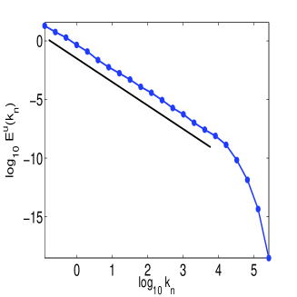
Figure 1: (Color online) Log-log plot of the fluid kinetic energy $E^{u}(k_{n})$ versus the wavenumber $k_{n}$ (blue filled circle joined by the continuous line) from our shell model studies. The thick black line indicates the K41 scaling.

We begin by describing results from our numerical simulations of the shell model for the SBF mixture. In our simulations the shell number is chosen such that $1\leq n\leq N$, where $N=22$ is the total number of shells and we use the boundary conditions $u_{n}=\psi_{n}=b_{n}=0\forall n<1$ or $\forall n>N$. We use a second-order Adams-Bashforth method to solve the equations, a time step $\delta t=10^{-4}$ and $\nu=\eta=10^{-8}$ in all our simulations. We choose a Gaussian, stochastic forcing on the fourth shell ($n=4$) to drive the system to a statistically steady state. Although in most studies of shell models, a deterministic force is used, we chose a stochastic forcing to make our shell model simulations consistent with our DNS. A snapshot of the fluid kinetic energy spectrum, obtained from our shell model studies, which gives a good indication of the extent of the inertial range obtained, are shown in Fig. 1 with the K41 scaling indicated by the thick black line. The extent of scaling, a little over 3 decades, is typical of such shell models and which allows measurements of scaling exponents with a higher degree of precision and confidence than in most DNS  raynjp . We show in Table 1 our equal-time scaling exponents $\psi$ (column 2), $b$ (column 3) and $u$ (column 4) fields; these exponents are calculated by using ESS, with respect to the third-order structure functions, for 50 different statistically independent statistically steady state configurations and quote the mean of these as our exponents and the standard deviation as the error-bars. We show the exponents for the velocity (red star) and the concentration field (red filled-circle), in Fig. 2 and for the gradient of the concentration field (red star), in Fig.  3, as a function of $p$; it is clear from the figures that there is clear multiscaling of the exponents associated with $u$ (see Fig. 2 , red star) and $b$ (see Fig. 3 , red star) and that the two agree with each other within error-bars (compare columns 3 and 4 in Table 1). In contrast, the exponents for $\psi$ (see Fig. 2 , red filled-circle) shows simple scaling and is indistinguishable, within error-bars, from the K41 prediction.

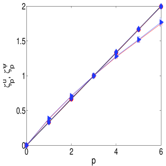
Figure 2: (Color online) Plots of $\zeta_{p}^{u}$ with error bars from our $128^{3}$ DNS (blue triangle) and shell model (red star), $\zeta_{p}^{\psi}$ with error bars from our $128^{3}$ DNS (blue diamond) and shell model (red filled-circle), and K41 scaling (thick black line) versus $p$. The lines connecting the data points from our simulations are a guide to the eye. The data from our DNS (upto $1\leq p\leq 6$) and shell model (shown for $1\leq p\leq 6$) are almost indistinguishable from each other upto $p=6$.

Figure 3: (Color online) Plots of $\zeta_{p}^{b}$ with error bars from our $128^{3}$ DNS (blue triangle) and shell model (red star), and K41 scaling (thick black line) versus $p$. The lines connecting the data points from our simulations are a guide to the eye. The data from our DNS (upto $1\leq p\leq 6$) and shell model (shown for $1\leq p\leq 6$) are almost indistinguishable from each other upto $p=6$.

How much of our results from the shell model studies, as described above, carries over to the actual Direct Numerical Simulations of the SBF mixture? We now describe the results obtained from our pseudospectral studies of the randomly forced symmetric binary fluid mixture equations (Eqs.3 and 4) and compare them with those obtained from the numerical solutions of our shell models. In our DNS, we keep $y=4$, corresponding to K41 spectra for the $\bf u$ and $\bf b$ fields, we use resolutions of $96^{3}$ and $128^{3}$ with a cubic box of linear size $L=2\pi$, and periodic boundary conditions. Our numerical scheme is identical to that in Ref. asain-prl . We use hyperviscosity and hyperdiffusivity together with ordinary viscosity and diffusivity. For the resolution $128^{3}$, we are able to achieve Taylor microscale Reynolds number $Re_{\lambda}\sim 150$. In Fig 4, we show a log-log plot of the fluid kinetic energy spectrum obtained from our DNS. Although our Reynolds number is not very high, we do obtain an inertial range close to three-quarters of a decade as can be seen in the figure. In the NESS obtained from these DNS we calculate the exponents $\zeta_{p}^{a}$, by using ESS with respect to the third-order structure function, from log-log plots of ${\mathcal{S}}_{p}^{a}(r)$ versus ${\mathcal{S}}_{3}^{a}(r)$ ($a=u_{i},b_{i},\psi$). From such plots, we use a modified local slope approach to obtain the equal-time exponents : We calculate the exponents over various ranges within the inertial range; we quote the mean as our exponent and the standard deviation as the error-bar. We find that : (i) The exponents $\zeta_{p}^{u}$ (Fig. 2, blue triangle) and $\zeta_{p}^{b}$ (Fig. 3, blue triangle) display multiscaling very similar to that in fluid turbulence: $\zeta_{2}^{m}/\zeta_{3}^{m}>2/3,\,\zeta_{p}^{m}/\zeta_{3}^{m}<p/3,\,p>3,\,m=u,b$, and, $\zeta_{p}^{u}/\zeta_{3}^{u}$ and $\zeta_{p}^{b}/\zeta_{3}^{b}$ are equal to each other within our error-bars (compare columns 6 and 7 in Table 1); and (ii) $\zeta_{p}^{\psi}/\zeta_{3}^{\psi}\approx p/3$ (Fig. 2, blue diamond). In addition, we calculate the normalized probability distribution function (PDF) $P[\delta a(r)]$ ($a=u_{i},b_{i},\psi$) for $r/\eta_{d}=7.7$ (see Fig.  5). We find $P[\delta u(r)]$ and $P[\delta b(r)]$ are nearly overlapping and have much longer tails than $P[\delta\psi(r)]$. Furthermore, $P[\delta\psi(r)]$ is well represented by a Gaussian of unit variance. In Fig. 6 we show plots of $P[\delta\psi(r)]$ versus $\delta\psi(r)$ for three different separations $r/\eta_{d}=7.7,\,23.2,\,26.2$ in the inertial range. A Gaussian of unit variance is again shown for comparison. We find that for all values of $r$, the plots overlap with each other and with the Gaussian. Also similar PDF plots for $u$ (Fig. 7 and $b$ (Fig. 8, for three different separations $r=/\eta_{d}=7.7,\,23.2,\,26.2$ not only show a marked departure from a Gaussian (as indicated by a continuous dark blue line) as was seen in Fig. 5, but also no collapse of the curves for different $r$ (unlike the case for $\psi$). These PDFs further strengthen and provide compelling evidence for our main results (i) and (ii) above. We present, in Table 1, the multiscaling exponents $\zeta_{p}^{\psi}$ (column 5), $\psi_{p}^{b}$ (column 6), and $\psi_{p}^{u}$ (column 7) from our DNS. We have checked that our results from the two different resolutions for the DNS agree with each other within error bars.

Given our modest resolution for our DNS, it is useful to examine how far we are justified in calculating moments up to order 6. It is well known that for higher order moments, the large contributions from the tails of the PDFs make statistical convergence progressively poor. In order to study statistical convergence, a good prescription is to examine the convergence of the moments of the differences of the velocity and the concentration fields  gotoh . Hence we study the bulk contributions $C_{6}[\delta a]$ to the sixth-order structure function (the highest order for which we present results in this paper) $S_{6}^{a}(r)$ ($a=\psi,\,u)$ defined as: $C_{6}(x)=\int_{0}^{x}x^{6}p(x)$ where $x=\delta\psi(r)$ or $\delta u$ (all suitably normalised), and $p(x)$ is the PDF of the same, respectively. In Fig. 9, we show a plot of $C_{6}[\delta\psi(r)]$ versus $\delta\psi(r)$ for two different $r=26.2\eta_{d}$ (black) and $7.7\eta_{d}$ (red): The two curves overlap, as is expected for a Gaussian form for $P[\delta\psi(r)]$ for various different values of $r$. In Fig. 10 we show a similar plot for $C_{6}^{u}[\delta u(r)]$ for the same two $r$ as before. Due to the non-Gaussian nature of $P[\delta u(r)]$, the two curves for two different $r$ do not overlap. These plots strongly display statistical convergence of the corresponding sixth-order moments. We obtain similar convergence for the gradient of the concentration field which we do not show here.

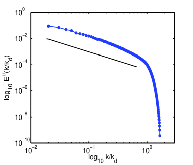
Figure 4: (Color online) Log-log plot of $E^{u}(k)$ versus $k/k_{d}$ (blue *) from our DNS studies (see text). $k_{d}\sim 98$ is the dissipation scale wavenumber here. The thick black line indicates the K41 scaling.

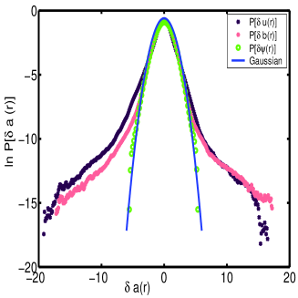
Figure 5: (Color online) Semilog plots of the probability distributions $P[\delta u(r)],\,P[\delta b(r)]$ and $P[\delta\psi(r)]$ versus $r$ in the inertial range, averaged over both time and the Cartesian components, from our DNS; a Gaussian distribution (blue continuous line) is shown for comparison.

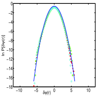
Figure 6: (Color online) Semilog plots of normalized probability distributions $P[\delta\psi(r)]$ as functions of $\delta\psi(r)$ for three different separations $r$ in the inertial range. A semilog plot of normalized Gaussian is shown for comparison. All plots are overlapping (see text).

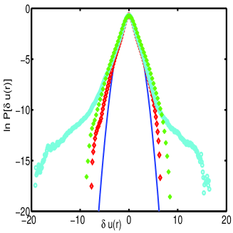
Figure 7: (Color online) Semilog plots of normalized probability distributions $P[\delta u(r)]$ as functions of $\delta u(r)$ for three different separations $r$ in the inertial range. A semilog plot of normalized Gaussian is shown for comparison (see text). The values of $r$ increases going inwards.

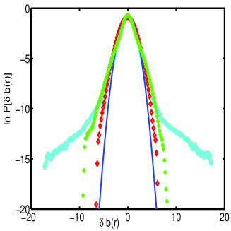
Figure 8: (Color online) Semilog plots of normalized probability distributions $P[\delta b(r)]$ as functions of $\delta b(r)$ for three different separations $r$ in the inertial range. A semilog plot of normalized Gaussian is shown for comparison (see text). The values of $r$ increases going inwards.

IV Conclusion

In summary, then, in this paper we have investigated the scaling and multiscaling properties of a turbulent symmetric binary fluid mixture via detailed numerical simulations. We find that ${\mathcal{S}}_{p}^{u,b}(r)$ exhibit multiscaling similar to fluid turbulence in the inertial range, whereas ${\mathcal{S}}_{p}^{\psi}(r)$ exhibit simple $p/3$ K41-scaling (within error bars). Moreover, the probability distributions $P[\delta u(r)]$ and $P[\delta b(r)]$ are nearly overlapping and have tails longer than that of $P[\delta\psi(r)]$ for $r$ in the inertial range. We also propose a new shell model for the gradient of the concentration field and numerically solve it as well as the shell model for scalar concentration field. Our results from our shell models are in agreement with our DNS studies. Our results are $3d$ analogues of those of Ref. celani , where simulations with particles in $2d$ flows were used to show that the structure functions of the concentration field for the SBF problem do not multiscale. The results from both our DNS of the SBF equations and shell-model studies are complementary to and agree well with each other and bring out the multiscaling of the velocity and concentration gradient fields and simple scaling of the concentration field. The validity of these conclusions is strengthened not only by the reliability of the scaling ranges usually associated with the measurement of equal-time structure functions in shell models, but also by the convincing PDFs that we obtain for various quantities in our DNS and the clear evidence of statistical convergence which justifies measurements of equal-time exponents upto order 6 in our DNS.

Our results may be explained from the analytical framework based on symmetry arguments developed in Ref. abhik , where it has been shown that the presence of an additional continuous symmetry (kind of a gauge symmetry), not present in the passive scalar turbulence model, is responsible for the simple scaling behaviour of $\zeta_{p}^{\psi}$. It would be interesting to investigate the properties of the turbulent NESS of SBF at low temperature, below the consolute point, when instabilities leading to phase separation competes with turbulent mixing. Work is in progress in this direction. Finally, our results may be tested in experiments similar to Ref. war .

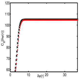
Figure 9: (Color online) Convergence of the sixth-order accumulated moment $C_{6}[\delta\psi(r)]$ versus $\delta\psi(r)$ for two different separations $r=26.2\eta_{d}$ (black) and $7.7\eta_{d}$ (red) in the inertial range. The two curves overlap (see text).

Figure 10: (Color online) Convergence of the sixth-order accumulated moment $C_{6}[\delta u(r)]$ versus $\delta u(r)$ for two different separations $r=26.2\eta_{d}$ (black, bottom) and $7.7\eta_{d}$ (red, top) in the inertial range. The two curves do not overlap (see text).

One of the authors (AB) gratefully acknowledges MPG(Germany)-DST(India) for partial financial support through the Partner Group program.

order$(p)$ $\zeta^{\psi,{\rm shell}}_{p}$ $\zeta^{b,{\rm shell}}_{p}$ $\zeta^{u,{\rm shell}}_{p}$ $\zeta^{\psi,{\rm DNS}}_{p}$ $\zeta^{b,{\rm DNS}}_{p}$ $\zeta^{u,{\rm DNS}}_{p}$ 1 0.3334 $\pm$ 0.0001 0.3671 $\pm$ 0.0001 0.378 $\pm$ 0.005 0.334 $\pm$ 0.001 0.372 $\pm$ 0.009 0.385 $\pm$ 0.009 2 0.6660 $\pm$ 0.0009 0.698 $\pm$ 0.005 0.707 $\pm$ 0.007 0.677 $\pm$ 0.001 0.70 $\pm$ 0.01 0.710 $\pm$ 0.009 3 1.0000 1.0000 1.0000 1.000 1.000 1.000 4 1.334 $\pm$ 0.002 1.277 $\pm$ 0.009 1.27 $\pm$ 0.01 1.340 $\pm$ 0.002 1.280 $\pm$ 0.009 1.28 $\pm$ 0.01 5 1.665 $\pm$ 0.005 1.54 $\pm$ 0.02 1.51 $\pm$ 0.02 1.671 $\pm$ 0.006 1.55$\pm$ 0.01 1.52 $\pm$ 0.04 6 1.995 $\pm$ 0.009 1.78 $\pm$ 0.03 1.75 $\pm$ 0.03 1.997 $\pm$ 0.008 1.78 $\pm$ 0.01 1.77 $\pm$ 0.06

Table 1: We show the various equal-time, order-$p$ exponents obtained from our shell model (indicated by the superscript shell) and DNS (indicated by the superscript DNS) studies. By comparing the corresponding columns, we find an agreement between the exponents obtained from DNS and the ones obtained from our shell models.

References

- (1) U. Frisch, Turbulence: The Legacy of A.N. Kolmogorov, Cambridge University Press, Cambridge (1995).
- (2) G. Falkovich, K. Gawedzki and M. Vergassola, Rev. Mod. Phys. 73, 913 (2001).
- (3) P.C. Hohenberg and B.I. Halperin, Rev. Mod. Phys. 49, 435 (2004) and references therein.
- (4) P.M. Chaikin and T.C. Lubensky, Principles of Condensed Matter Physics (Cambridge University, Cambridge, England, 2004).
- (5) A.N. Kolmogorov, Dokl. Akad. Nauk SSSR 30, 301 (1941).
- (6) A.N. Kolmogorov, Dokl. Akad. Nauk SSSR 31, 538 (1941).
- (7) R. Kraichnan, Phys. Fluids 11, 945 (1968).
- (8) R. Kraichnan, Phys. Rev. Lett. 72, 1016 (1994).
- (9) R. Kraichnan, Phys. Rev. Lett. 78, 4922 (1997).
- (10) A. M. Obukhov, Izv. Akad. SSSR, Serv. Geogr. Geofiz. 13, 58 (1949).
- (11) S. Corrsin, J. Appl. Phys. 22, 469 (1951).
- (12) H. L. Swinney et al., Phys. Rev. A, 8, 2586 (1973).
- (13) A. Celani et al, Phys. Rev. Lett., 89, 234502 (2002).
- (14) A. Basu, J. Stat. Mech., L09001 (2005).
- (15) R. Ruiz and D. R. Nelson, Phys. Rev. A, 23, 3224 (1981).
- (16) M. K. Nandy et al., J. Phys. A, 31, 2621 (1998).
- (17) M. Chertkov et al, Phys. Rev. E, 52, 4924 (1995); M. Chertkov et al, Phys. Rev. Lett., 76, 2706 (1996); K. Gawedzki and A. Kupiainen, Phys. Rev. Lett., 75, 3834 (1995); D. Bernard et al. Phys. Rev. E, 54, 2564 (1996); L. Ts. Adzhemyan et al. Phys. Rev. E, 58, 1823 (1998).
- (18) D. Montgomery, in Lecture Notes on Turbulence, edited by J. R. Herring and J. C. McWilliam (World Scientific, Singapore, 1989); D. Biskamp, in Nonlinear Magnetohydrodynamics, edited by W. Grossman et al. (Cambridge University Press, Cambridge, England, 1993).
- (19) In a renormalization group language fields and have the same canonical dimensions when the respective equations of motion are driven by noises having variances with same spatial scaling.
- (20) A. Basu et al, Phys. Rev. Lett.81, 2687 (1998).
- (21) V. Yakhot and S.A. Orszag, Phys. Rev. Lett., 57, 1722 (1986); J.K. Bhattacharjee, J. Phys. A, 21, L551 1988.
- (22) C.Y. Mou and Weichman, Phys. Rev. Lett., 70, 1101 (1993); G.L. Eyink, Phys. Fluids, 6, 3063 (1994).
- (23) Z. S. She and E. Leveque, Phys. Rev. Lett., 72, 336 (1994).
- (24) R. Benzi et al., Phys. Rev. E, 48, R29 (1993); S. K. Dhar et al, Phys. Rev. Lett., 78, 2964 (1997); S. Chakraborty et al., J. of Fluid Mech., 649, 275 (2010).
- (25) E. B. Gledzer, Sov. Phys. Dokl., 18, 216 (1973); K. Ohkitani and M. Yamada, Prog. Theor. Phys., 81, 329 (1989).
- (26) S.S. Ray et al., New J. Phys., 10, 033003 (2008).
- (27) M. H. Jensen and P. Olesen, Physica D, 111, 243 (1998).
- (28) A. Sain et al, Phys. Rev. Lett., 81, 4377 (1998).
- (29) T. Gotoh, D. Fukayama, and T. Nakano, Phys. Fluids, 14, 1065 (2002).
- (30) R. E. G. Poorte and A. Biesheuvel, J. Fluid Mech., 461, 127 (2002), A. Gylfason and Z. Warhaft, Phys. Fluids, 16, 4012 (2004), and references therein.