Ginwidth=7.75cm,clip=true
Towards a density functional description of liquid pH2
Abstract
A finite-temperature density functional approach to describe the properties of parahydrogen in the liquid-vapor coexistence region is presented. The first proposed functional
is zero-range, where the density-gradient term is adjusted so as to reproduce the
surface tension of the liquid-vapor interface at low temperature.
The second functional is finite-range and, while it is fitted to reproduce bulk pH2 properties only,
it is shown to yield surface properties in good agreement with
experiments. These functionals are used to study the surface thickness of the liquid-vapor
interface, the wetting transition of parahydrogen on a planar Rb
model surface, and homogeneous cavitation in bulk liquid pH2.
Keywords: atomic and molecular clusters, molecular hydrogen and isotopes, density functional theory.
IFIC (CSIC and Universidad de Valencia). Apdo. 22085, 46071 Valencia, Spain.
Dipartimento di Fisica, ‘G.Galilei’, Università di Padova, via Marzolo 8, I-35131 Padova, Italy and CNR-IOM-Democritos, I-34014 Trieste, Italy.
Departament ECM, Facultat de Física, and IN2UB, Universitat de Barcelona. Diagonal 647, 08028 Barcelona, Spain.
1 Introduction
Under normal conditions of pressure and temperature hydrogen is a gas formed by H2 molecules. The molecule exists in two isomeric forms, para (pH2) and ortho (oH2), which differ in the coupling of their nuclear spins: antiparallel () and parallel (), respectively. At low temperatures, near the boiling point (20.3 K), hydrogen can be catalyzed in nearly all parahydrogen.
The purpose of this paper is to present a free energy density functional for liquid parahydrogen. Our approach is largely inspired by density functional methods currently employed to study liquid helium at very low temperature.[1, 2, 3] Indeed, the pH2 molecule and the 4He atom have in common that both are spinless bosons subject to a weak van der Waals interaction. While helium remains liquid down to K, the stable low-temperature bulk phase of hydrogen, in spite of the lighter mass of the pH2 molecule, is an hpc solid. This is a consequence of the attractive interaction between two pH2 molecules, which is a factor of four stronger than the He-He one. The density functional for parahydrogen presented here is valid in the temperature range 14 K 32 K, i.e., between the triple (13.8 K) and nearly the critical point (32.938 K). While the functional is still reliable in the neighborhood of the liquid-vapor coexistence region, the extrapolation at lower temperatures to study, for instance, the metastable overcooled liquid, still remains an open question.
Ginzburg and Sobyanin[4] have suggested that liquid parahydrogen could exhibit superfluidity, analogously to liquid helium, below some critical temperature that they estimated to be at around 6 K. To have superfluid pH2 it is therefore necessary to bring the liquid below its saturated vapor pressure curve. Attempts to produce a superfluid by supercooling the normal liquid below the triple point have been insofar unsuccessful.[5] As a possible way to stabilize the liquid phase of pH2 at low temperatures several authors have considered restricted geometries in order to reduce the effective attraction between molecules. Indeed, the lowering of the melting point compared to the bulk liquid is a well-known and rather general phenomenon in clusters, see e.g. Ref. ([6]). Path integral Monte Carlo (PIMC) simulations by Sindzingre et al.[7] predicted that (pH2)N clusters with and 18 molecules are superfluid below about 2 K. This prediction motivated two experiments[8, 9, 10] and a much larger number of theoretical studies on small (pH2)N clusters, see e.g. Refs. ([11, 12, 13]) and references therein. Concerning two-dimensional pH2 systems, PIMC calculations of films have found that introducing some alkali metal atoms stabilizes a liquid hydrogen phase which undergoes a superfluid transition below K.[14] Moreover, experiments on adsorption of H2 films on alkali metals substrates[15, 16] have reported the existence of a wetting transition, analogous to what is known for helium.
A density functional (DF) for liquid parahydrogen at finite temperatures could help to describe these phenomena. Indeed, DF methods have become increasingly popular in recent years as useful computational tools to study the properties of classical and quantum inhomogeneous fluids,[17] especially for large systems for which these methods provide a good compromise between accuracy and computational cost, yielding results in agreement with experiment or with more microscopic approaches.
A first step in that direction was made by Boninsegni and Szybisz,[18] who constructed a density functional to study the low temperature energetics and structural behavior of H2 films adsorbed on Cs and Li substrates. They fitted the DF parameters by using as input experimental informations from the solid phase, such as the ground state equilibrium density, the sublimation energy, and the bulk modulus. Our approach is based on a different strategy, as its aim is to provide a DF that can be reliably used in the liquid-vapor coexistence region.
This paper is organized as follows. In Sec. 2 we describe the density functional for liquid parahydrogen in two versions, neglecting or not finite-range effects. The validity of the DF is assessed in Sec. 3 by comparing the calculated surface tension with experiment. The DF is thus used to study the wetting of a Rb planar surface by pH2, and the results are compared to those obtained by Quantum Monte Carlo simulations. As a final application, in Sec. 4 we describe homogeneous cavitation in liquid pH2. A brief summary and outlook are presented in Sec. 5.
2 The density functional
Following the procedure previously employed for liquid 4He, in particular the works of Guirao et al.,[19] Dalfovo et al.,[2] and Ancilotto et al.,[20] we present first a density functional for bulk liquid parahydrogen. The extension to inhomogeneous liquids will be considered in the next section. In the most general form, the free energy of a Bose system is assumed to be a DF, which we write as
| (1) |
where is the free energy density for an ideal Bose gas, and is the correlation energy density, which incorporates the dynamic correlations induced by the interaction. The number of pH2 molecules per unit volume is denoted by .
2.1 The non-interacting part
The expression for at is given in textbooks. Following Ref. ([21]) it can be written as
| (2) |
where
| (3) |
is the pH2 thermal wavelength, is the H2 mass, and the fugacity is defined as:
| (4) |
where is the root of the equation . In the above equations, . In the following we shall use units such that the Boltzmann constant is one, so that energy is measured in K. In these units 24.0626 K Å2.
2.2 The correlation part
Once the functional Eq. (1) is defined, a complete thermodynamical description of the bulk liquid can be achieved. In particular, the chemical potential and the pressure are given by
| (5) |
and
| (6) |
In the next subsections we propose a phenomenological expression for the correlation energy density, inspired by previous works on liquid helium, which contains a few adjustable parameters which are fixed so as to reproduce selected experimental properties of the liquid from the data collected by McCarthy et al.[22] or the more recent compilation by Leachman et al.[23] In fact, the latter compilation has been summarized in terms of a rather complex parametrization of the bulk liquid pH2 free energy density which reproduces satisfactorily the available experimental data between the triple and the critical points in a wide range of pressure values.
We present here a simpler yet less accurate functional that has the advantage of being easier to generalize to finite systems (drops, liquid pH2 in confined geometries) and presents a more conventional separation into kinetic and potential terms. This may be of interest for other applications, such as computing the excitation spectrum as well as the static and dynamic responses of these systems.[3] Besides, the present DF could in principle be extrapolated to lower temperatures near , one of our medium-term goals.
2.2.1 Zero-range
We consider a polynomial in powers of the density to represent the correlation part of the free-energy density
| (7) |
For a given value of , there are thus four free parameters. With this form, other quantities such as the chemical potential , the pressure , and the speed of sound , can be written as
where, for the sake of simplicity, we have omitted the -dependence in the parameters.
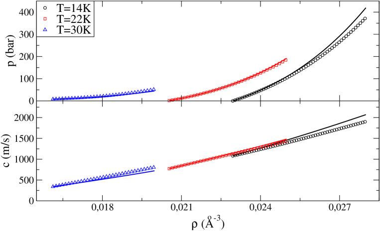
These parameters are fixed by the following strategy. At a given , we determine the liquid-vapor equilibrium by imposing the equality between pressures and chemical potentials. The liquid and vapor densities are experimentally known.[23] This provides two conditions. The other two conditions are the fitting of the pressure and speed of sound of the liquid phase at the saturated vapor pressure to the corresponding experimental values.[23] The resulting parameters are given in Table 1. We shall refer to them as the DFpH2 set.
In Fig. 1 the experimental and calculated pressure and speed of sound as a function of for three values of are compared. For each , the first density value shown is that of the liquid at the liquid-vapor coexistence, where and coincide by construction with the experimental values. It is worthwhile seeing that the DFpH2 parametrization can be safely used for densities well above those of the liquid at the saturation vapor pressure.
2.2.2 Finite-range
The functional Eq. (7) is a zero-range one, and it cannot account for inhomogeneities or finite size effects induced by strong density compression. Inspired in the way this problem has been addressed in the case of liquid 4He,[2] we derive from Eq. (7) a finite-range density functional with the following prescriptions. On one hand, the term in is replaced with
| (8) |
where represents the H2-H2 pair interaction screened at short distances
| (9) |
and otherwise. We have used the Lennard-Jones parameters K and Å, which are slightly different from the standard ones (34.2 and 2.96, respectively). The value of is fixed by the condition
| (10) |
The values of are given in the last column of Table 1.
On the other hand, a coarse-grained density is introduced in the remaining terms of the correlation part Eq. (7):
| (11) |
where
| (12) |
with
| (13) |
and otherwise. For the reasons explained in Sec. 3.2, we have taken .
3 Surface and interface properties
Once the DF parameters have been adjusted to reproduce the bulk behavior of liquid pH2 at finite temperatures, the predicted surface and interface properties provide a significant test about its validity. We present in this section the results of a series of calculations aimed at showing that our proposed DF can indeed be reliably used to study finite temperature properties of inhomogeneous pH2 systems, such as a free-standing fluid-vapor interface or liquid pH2 adsorbed on a solid surface.
We have first computed the liquid-vapor surface tension of pH2 as a function of temperature, and compared our results with the experimental data of Ref. ([22]). We obtain a liquid-vapor interface by minimizing the DF with the appropriate boundary conditions, corresponding to a planar liquid pH2 film in equilibrium with its own vapor. In this case the solution depends only on the coordinate normal to the surface, and provides the equilibrium density profile . From the knowledge of one can extract values for the surface tension . We distinguish in the following two different approaches used to compute this quantity, the first one being based on the zero-range DF described in Sec. 2.2.1, and the second one on the more accurate but computationally more expensive non-local, finite-range DF described in Sec. 2.2.2.
3.1 The pH2 surface tension from zero-range DF calculations
Our starting point is the zero-range free energy density functional
| (14) |
This is the simplest extension of Eq. (1) in Sec. 2 including the first two terms in a gradient expansion to account for density inhomogeneities. We make here the usual choice[2] for the kinetic energy term, while we fix to the value K Å5, which allows to reproduce the experimental surface tension at K.[22]
With such a form for the free energy density, the surface tension turns out to be[24]
| (15) |
being the asymptotic (constant) density values on the liquid and vapor side of the interface, respectively.
We show in Fig. 2 our results for the pH2 surface tension. The open squares correspond to the calculated points, while the dotted line shows the experimental result from Ref. ([22]). It appears that, once the DF parameter is fixed to reproduce the value at a given temperature, say K, the predictions for are quite accurate in the whole range of temperatures between the triple and near the critical point.
3.2 The pH2 surface tension from finite-range DF calculations
We use here the finite-range description of the free energy density functional of pH2, as discussed in Section 2.2.2. Concerning the coarse-grained density defined in Eq. (12), the empirical prescription is the one which gives optimum agreement between the calculated and measured values for .
We use a slab geometry in our calculations, with periodic boundary conditions whereby a thick planar liquid film is in contact with a vapor region. Our calculations, which are effectively one-dimensional, are performed within a region of length . Rather large values of and of the film thickness (no to be confused with the thickness of the liquid-vapor interface) are necessary for well converged calculations (typically Å and Å), in order to let the system spontaneously reach (i) the bulk liquid density in the interior of the film and (ii) the bulk vapor density in the region outside the film.
The equilibrium density profile of the fluid at the interface is determined from the variational minimization of the grand potential, leading to the following Euler-Lagrange (EL) equation:
| (16) |
where the effective potential is defined as the functional derivative of the free energy density,[2] and the value of the chemical potential is fixed by the normalization condition to the total number of H2 molecules per unit area, .
In Fig. 3 we show some selected equilibrium density profiles around the liquid-vapor interface calculated using the finite-range DF. As expected, the width of the interface increases monotonically with temperature. Density profiles for H2 have been obtained in Ref. ([26]) using the Silvera-Goldman potential[25] within a molecular simulation of the liquid-vapor interface. However, the rather thin liquid slab used there is probably insufficient to properly describe the liquid-vapor interface. For this reason we do not attempt a quantitative comparison between our calculated profiles and those reported in Ref. ([26]).
The liquid-vapor surface tension can be directly computed from the definition once the equilibrium density profiles have been obtained. In the previous expression, is the grand potential, is the saturated vapor pressure at temperature , is the volume of the system, and is the surface area. For the one-dimensional problem considered here, one has:
| (17) |
The pressure can be conveniently calculated from the definition . A factor appears in the previous equation to account for the two free surfaces delimiting the liquid film in our slab geometry calculations. The surface tension obtained from the finite-range DF is also shown in Fig. 2 as full squares. The overall agreement with the available experimental data[22] is quite satisfactory.
We show in Fig. 4 the results obtained for the thickness of the liquid-vapor interface. We define the thickness as the distance across the interface between the points at which the fluid density changes from 0.9 to 0.1 times that of the liquid at saturation for the corresponding and values. Open squares represent the values obtained using the zero-range DF, and full squares those obtained using the finite-range DF. The latter are our prediction for the thickness of the interface. Similarly to what occurs for liquid 4He,[2, 20] the thickness of the liquid-vapor interface obtained from the finite-range DF at low temperatures is about 2 Å smaller than that obtained from the zero-range DF.
3.3 Wetting properties: the pH2/Rb system
The existence and nature of the wetting transition[27] at a temperature above the triple point (and below the critical temperature) is known to be the result of a delicate balance between the interatomic potential acting among the atoms in the liquid and the atom-substrate interaction potential. When the latter dominates, the fluid tends to wet the surface.
When a first order transition from partial to complete wetting occurs at a temperature above the triple-point (and below the bulk critical temperature), then a locus of first-order surface phase transitions must extend away from the liquid-vapor coexistence curve, on the vapor side. At the thickness of the adsorbed liquid film increases continuously with pressure, but the film remains microscopically thin up to the coexistence pressure , and becomes infinitely (macroscopically) thick just above it. At temperatures , being the prewetting critical temperature, the thin film grows as the pressure is increased until a transition pressure is reached. At this pressure a thin film is in equilibrium with a thicker one, and a jump in coverage occurs as increases through . At still higher pressures this first order transition is followed by a continuous growth of the thick film which becomes infinitely thick at .[28, 29]
Wetting transitions have been observed for quantum fluids (helium and hydrogen) on alkali metal surfaces. In particular, H2 on Rb surface shows a wetting transition.[15] This system has been addressed by finite temperature quantum simulations in Ref. ([30]), where a first-order wetting transition was indeed found to occur. The value found for the wetting temperature, K was higher than the experimental value K.[15] The disagreement has been attributed to the fact that the interaction potential used to simulate the fluid-surface interaction was probably too weakly attractive. We are not concerned here in reproducing the experimental value for but rather to compare the prediction of our finite-range DF approach against an accurate benchmark, i.e. the virtually exact Quantum Monte Carlo results reported in Ref. ([30]). The external potential ( is the coordinate normal to the surface plane) used in Ref. ([30]) to describe the H2/Rb surface interaction is a semi-ab initio one.[31] In order to make a proper comparison with the results of Ref. ([30]) we have used the same atom-surface potential employed there, and calculate within finite-range DF theory the wetting temperature for the pH2/Rb system.
The free energy finite-range functional for pH2 described in Sec. 2.2.2 must be augmented by a term describing the interaction (per unit surface) of the pH2 fluid with the Rb surface, , and the equilibrium density profile of the fluid adsorbed on the surface is determined by direct minimization of the density functional with respect to density variations, which yields an equation similar to Eq. (16) with an extra potential term arising from . Details on the procedure can be found e.g., in Ref. ([32]) and references therein.
We show in Fig. 5 a set of calculated density profiles for different temperatures. We fix in our calculations the pressure (equivalently, the chemical potential) just below the bulk liquid saturation pressure, and increase the temperature. The abrupt (first order) change in the amount of liquid adsorbed on the surface shown in Fig. 5 when is just above K is a clear signature of the pre-wetting transition very close to saturation. We thus take as our prediction for the value K. This value compares well with the one found by Quantum Monte Carlo calculations.[30]
4 Cavitation
Another application of the density functionals described in Sec. 2 is the study of thermal homogeneous cavitation in liquid pH2. It can be straightforwardly extended to the case of nucleation of pH2 droplets in a supersaturated parahydrogen vapor. From the experience gathered in similar 4He studies, it is enough to use the zero-range DF for this application. We refer the reader e.g., to Refs. ([33, 34, 35, 36, 37]) and references therein for a general discussion of similar work carried out for liquid helium.
It is well know that phase transitions take place in the coexistence region of different phases of homogeneous systems, and that it does not always happen under equilibrium conditions. Indeed, as the coexisting phase forms, the free energy of the system is lowered, but the original phase can be held in a metastable state close to the equilibrium transition point. The metastable state is separated from the stable state by a thermodynamic barrier that can be overcome by statistical fluctuations.
Cavitation consists in the formation of bubbles in a liquid held at a pressure below the saturation vapor pressure at the given temperature. In this case, cavitation is a thermally driven process. The formation of the vapor phase from the metastable liquid proceeds through the formation of a critical bubble, whose expansion cannot be halted as its energy equals the thermodynamic barrier height. A very simple estimate of the radius of this critical bubble is provided by the thin wall model, which consists in treating the bubble as a spherical cavity of sharp surface and radius filled with vapor at the saturated vapor pressure, . The barrier for creating a bubble of radius is the result of a balance between surface and volume energy terms
| (18) |
where is the difference between the applied pressure and , and can be positive and negative as well. This barrier has thus a maximum at a critical radius . Taking dyne/cm at = 14 K,[22] and bar (the pH2 spinodal pressure at K), one gets Å.
The cavitation rate , i.e., the number of critical bubbles formed in the liquid per unit time and volume is given by
| (19) |
and the prefactor depends on the dynamics of the cavitation process. A precise knowledge of the prefactor is not crucial, since at given , the exponential term in Eq. (19) dramatically varies with in the pressure range of interest, thus making the determination of rather insensitive to its actual value.[34] We shall estimate as an attempt frequency per unit volume, namely , where is the Planck constant and is the volume of the critical bubble.
To determine the homogeneous cavitation pressure within DF theory, one has first to determine the critical bubble for and values corresponding to points lying within the liquid-vapor phase equilibrium region where bubbles may appear. This is done by solving the EL equation arising from the functional variation of the grand potential with respect to the pH2 particle density. The grand potential density is , where is the free energy per unit volume including surface terms arising from the bubble surface and kinetic energy contributions already discussed in Sec. 2.2.1, and is the chemical potential of the bulk liquid. The EL equation is solved imposing the physical conditions that and , where is the density of the metastable homogeneous liquid.
The nucleation barrier is obtained by subtracting the grand potential of the critical bubble from that of the homogeneous metastable liquid at the given and
| (20) |
where has no density gradient terms as it corresponds to the metastable homogeneous liquid. The above expression embraces the two limiting physical situations of a barrierless process when the system approaches the spinodal point, and of an infinite barrier process when the system approaches the saturation line. While the latter limit is well reproduced by the thin wall model, the former is not.[34, 36]
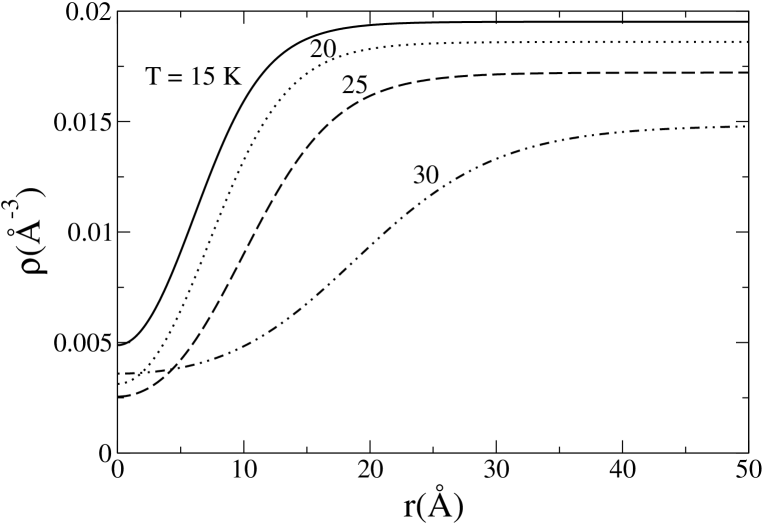
Figure 6 shows several density profiles for critical bubbles at selected values. For each temperature, we have chosen the pressure corresponding to the homogeneous cavitation value, see below. The radius of the critical bubble for K is similar to that obtained within the thin wall model at K.
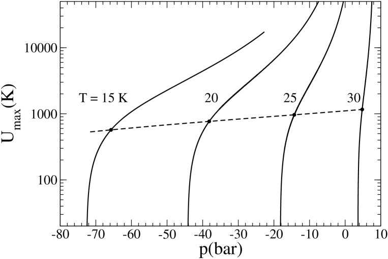
Figure 7 shows the barrier height of the critical bubble for selected values as a function of (solid lines). The divergence of as approaches the saturation line, as well as its disappearance at the spinodal line are clearly visible in the figure.
At a given temperature, there is an appreciable probability of cavitation occuring when reaches a value such that
| (21) |
where is the experimental volume times the experimental time. This defines the homogeneous cavitation pressure , an intrinsic property of the liquid that is determined by solving the above algebraic equation. To solve Eq. (21) one needs some experimental information. If the experiment were carried out as for liquid 4He,[38] cm3 s. Lacking of a better choice, this is the value we shall adopt here for parahydrogen.
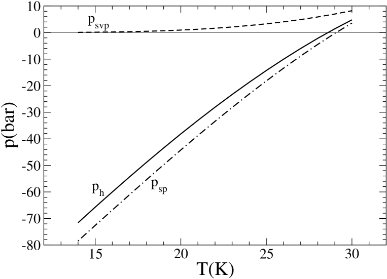
Figure 8 shows the homogeneous cavitation pressure as a function of . Also shown is the spinodal line and the saturation vapor pressure line . The three lines merge at the critical point. It can be seen that is negative up to K, meaning that a large tensile strength may be needed to produce cavitation. Notice that, as in 4He,[33, 34] the homogeneous cavitation pressure is just above the spinodal pressure.
Finally, we mention that the dashed line in Fig. 7 represents the barrier height at for the chosen value. It can be seen that these heights are in the 500-1000 K range for temperatures K.
5 Summary and outlook
In this work we have proposed a density functional that can be used to study the properties of parahydrogen in the liquid-vapor phase-diagram region and its neighborhood. We have used its zero-range version to address thermal homogeneous cavitation in the metastable liquid, and its finite-range version to predict the thickness of the liquid-vapor interface. We have shown that this finite-range DF predicts the surface tension of the liquid-vapor interface and the wetting properties of pH2 on planar Rb surfaces in satisfactory agreement with experiments and microscopic calculations, respectively.
Besides thermal cavitation, the existence of a finite temperature, finite-range DF makes it possible to improve the theoretical description of phenomena that hardly could be described using more fundamental approaches, as the study of electron bubbles in pH2.[39, 40] Large pure or doped parahydrogen drops at finite temperature could also be addressed provided the impurity-pH2 interaction is known, as well as extending the study of wetting to other substrates and/or geometries.
The present DF may be of interest for other applications, such as the calculations of the excitation spectra of pure or doped pH2 drops, as well as their static or dynamic responses. The extrapolation of the DF to temperatures near still remains an open question. We plan to study some of these phenomena in the future.
Acknowledgments
This work has been performed under Grants No. FIS2008-00421/FIS and FIS2007-60133 from DGI, Spain (FEDER), and Grant 2009SGR01289 from Generalitat de Catalunya.
References
- [1] Stringari, S.; Treiner, J. Phys. Rev. B 1987, 36, 16; J. Chem. Phys. 1987, 87, 5021.
- [2] Dalfovo, F.; Lastri A.; Pricaupenko, L.; Stringari, S.; Treiner, J. Phys. Rev. B 1995, 52, 1193.
- [3] M. Barranco, M.; Guardiola, R.; Hernández, S.; Mayol, R.; Pi, M. J. Low Temp. Phys. 2006, 142, 1.
- [4] Ginzburg, V.L.; Sobyanin, A.A. Sov. Phys. JETP Lett. 1972, 15, 242.
- [5] Maris, H.J.; Seidel, G.M.; Huber, T.E. J. Low Temp. Phys. 1983, 51, 471.
- [6] Alonso, J.A. Structure and Properties of Atomic Clusters. Imperial College Press: London, (2005).
- [7] Sindzingre, Ph.; Ceperley, D.M.; Klein, M.L. Phys. Rev. Lett. 1991, 67, 1871.
- [8] Grebenev, S.; Sartakov, B.; Toennies, J.P.; Vilesov A.F. Science 2000, 289, 1532.
- [9] Tejeda, G.; Fernández, J.M.; Montero, S.; Blume, D.; Toennies, J.P. Phys. Rev. Lett. 2004, 92, 223401.
- [10] Montero, S.; Morilla, J.H.; Tejeda, G.; Fernández, J.M. Eur. Phys. J. D 2009, 52, 31.
- [11] Warnecke, S.; Sevryuk, M.B.; Ceperley, D.M.; Toennies, J.P.; Guardiola, R.; Navarro J. Eur. Phys. J. D 2010, 56, 353.
- [12] Alonso, J.A.; Martínez, J.I. Handbook of Nanophysics. Vol 2: Clusters and Fullerenes, Sattler, K.D., Ed.; Taylor and Francis: Boca Raton, 2010.
- [13] Navarro, J.; Guardiola, R. Int. J. Quantum Chem 2011, 111, 463.
- [14] Gordillo, M.C.; Ceperley, D.M. Phys. Rev. Lett. 1997, 97, 3010.
- [15] Mistura, G.; Lee, H.C.; Chan, M.H.W. J. Low Temp. Phys. 1994, 96, 221.
- [16] Ross, D.; Taborek, T.; Rutledge, J.E. Phys. Rev. B 1998, 58, 4247
- [17] Evans, R. Liquids at interfaces, (Editors J. Charvolin, J. F. Joanny, and J. Zinn-Justin). Elsevier, (1989).
- [18] Boninsegni, M.; Szybisz L. J. Low Temp. Phys. 2004, 134, 315.
- [19] Guirao, A.; Centelles, M.; Barranco, M.; Pi, M.; Polls, A.; Viñas, X. J. Phys.: Condensed Matter 1992, 4, 667.
- [20] Ancilotto, F.; Faccin, F.; Toigo, F. Phys. Rev. B 2000, 62, 17035.
- [21] Huang, K. Statistical Mechanics, J. Wiley: New York, 1987, 2nd. edition.
- [22] McCarthy, R.D.; Hord, L.; Roder, H.M. National Bureau of Standards 1981, Monograph num. 168.
- [23] Leachman, J.W.; Jacobsen, R.T.; Penoncello, S.G.; Lemmon, E.W. J. Phys. Chem. Ref. Data 2009, 38, 721.
- [24] Barranco, M.; Pi, M.; Polls, A.; Viñas, X. J. Low Temp. Phys. 1990, 80, 77.
- [25] Silvera, I.F.; Goldman, V.V. J. Chem. Phys. 1978, 69, 4209.
- [26] Zhao, X.; Johnson, J.K.; Rasmussen, C.E. J. Chem. Phys. 2004, 120, 8707.
- [27] Cahn, J.W. J. Chem. Phys. 1977, 66, 3667.
- [28] Cheng, E.; Cole, M.W.; Dupont-Roc, J.; Saam, W.F.; Treiner, J. Rev. Mod. Phys. 1993, 65, 557.
- [29] Bonn, D.; Ross, D. Rep. Prog. Phys. 2001, 64, 1085.
- [30] Shi, W.; Johnson, J.K.; Cole, M.W. Phys. Rev. B 2003, 68, 125401.
- [31] Chizmeshya, A.; Cole, M.W.; Zaremba, E. J. Low Temp. Phys. 1998, 110, 677.
- [32] Ancilotto, F.; Barranco, M.B.; Hernández, E.S.; Pi, M. J. Low Temp. Phys. 2009, 157, 174.
- [33] Xiong, Q.; Maris, H.J. J. Low Temp. Phys. 1991, 82, 105.
- [34] Jezek, D.M.; Guilleumas, M.; Pi, M.; Barranco, M.; Navarro, J. Phys. Rev. B 1993, 48, 16582.
- [35] Pettersen, M.S.; Balibar, S.; Maris, H.J. Phys. Rev. B 1994, 49, 12062.
- [36] Barranco, M.; Guilleumas, M.; Pi, M.; Jezek, D.M. Microscopic Approaches to Quantum Liquids in Confined Geometries, E. Krotscheck and J. Navarro, editors. World Scientific: Singapore, (2002), p. 319.
- [37] Balibar, S. J. Low Temp. Phys. 2002, 129, 363.
- [38] Caupin, S.; Balibar, S. Phys. Rev. B 2001, 64, 064507.
- [39] Levchenko, A.A.; Mezhov-Deglin, L.P. JETP Lett. 1994, 60, 470.
- [40] Berezhnov, A.V.; Khrapak, A.G.; Illenberger, E.; Schmidt, W.F. High Temperature 2003, 41, 425.
| 14 | -5.39621105 | 2.25023742 | -1.20053135 | 2.79594232 | 2.98886735 |
|---|---|---|---|---|---|
| 15 | -5.28361552 | 2.15103496 | -1.14667549 | 2.70797035 | 2.93284836 |
| 16 | -5.18646074 | 2.07504193 | -1.10362936 | 2.63656153 | 2.90255249 |
| 17 | -5.10162915 | 2.01565556 | -1.06770278 | 2.57547938 | 2.88158016 |
| 18 | -5.02544156 | 1.96727851 | -1.03616377 | 2.52033226 | 2.86543169 |
| 19 | -4.95500617 | 1.92571884 | -1.00701996 | 2.46790257 | 2.85212913 |
| 20 | -4.88844024 | 1.88827147 | -0.978964063 | 2.41596399 | 2.84067446 |
| 21 | -4.82469889 | 1.85328416 | -0.951137931 | 2.36290741 | 2.83053490 |
| 22 | -4.76330170 | 1.81966306 | -0.922799978 | 2.30707709 | 2.82141283 |
| 23 | -4.70410834 | 1.78695682 | -0.893590816 | 2.24744238 | 2.81313315 |
| 24 | -4.64712668 | 1.75458070 | -0.862880207 | 2.18218726 | 2.80558079 |
| 25 | -4.59255499 | 1.72283140 | -0.830703205 | 2.11075548 | 2.79868923 |
| 26 | -4.54035421 | 1.69068884 | -0.795990139 | 2.03000386 | 2.79237811 |
| 27 | -4.49046505 | 1.65741296 | -0.757823418 | 1.93673005 | 2.78657987 |
| 28 | -4.44267216 | 1.62195349 | -0.714989528 | 1.82655914 | 2.78122146 |
| 29 | -4.39598018 | 1.58109948 | -0.664408250 | 1.68988952 | 2.77615776 |
| 30 | -4.34840634 | 1.52965533 | -0.601172851 | 1.51084983 | 2.77116004 |
| 31 | -4.29478440 | 1.45544413 | -0.514224892 | 1.25423884 | 2.76570856 |
| 32 | -4.21484337 | 1.31639928 | -0.367772398 | 0.809972555 | 2.75790923 |