Existence of random gradient states

Abstract

We consider two versions of random gradient models. In model A the interface feels a bulk term of random fields while in model B the disorder enters through the potential acting on the gradients. It is well known that for gradient models without disorder there are no Gibbs measures in infinite-volume in dimension $d=2$, while there are “gradient Gibbs measures” describing an infinite-volume distribution for the gradients of the field, as was shown by Funaki and Spohn. Van Enter and Külske proved that adding a disorder term as in model A prohibits the existence of such gradient Gibbs measures for general interaction potentials in $d=2$.

In the present paper we prove the existence of shift-covariant gradient Gibbs measures with a given tilt $u\in\mathbb{R}^{d}$ for model A when $d\geq 3$ and the disorder has mean zero, and for model B when $d\geq 1$. When the disorder has nonzero mean in model A, there are no shift-covariant gradient Gibbs measures for $d\geq 3$. We also prove similar results of existence/nonexistence of the surface tension for the two models and give the characteristic properties of the respective surface tensions.

T1Support by the TUM Institute for Advanced Study (TUM-IAS), by the Sonderforschungsbereich SFB — TR12—Symmetries and Universality in Mesoscopic Systems, and by the University of Bochum.

and

1 Introduction

1.1 The setup

Phase separation in $\mathbb{R}^{d+1}$ can be described by effective interface models for the study of phase boundaries at a mesoscopic level in statistical mechanics. Interfaces are sharp boundaries which separate the different regions of space occupied by different phases. In this class of models, the interface is modeled as the graph of a random function from $\mathbb{Z}^{d}$ to $\mathbb{Z}$ or to $\mathbb{R}$ (discrete or continuous effective interface models). For background and earlier results on continuous and discrete interface models without disorder, see, for example, BY , CD , CDM , DGI , FL , FS , gos and references therein. In our setting, we will consider the case of continuous interfaces with disorder as introduced and studied previously in EK and KO . Note also that discrete interface models in the presence of disorder have been studied, for example, in BK1 and BK2 . We will introduce next our two models of interest.

In our setting, the fields $\varphi(x)\in\mathbb{R}$ represent height variables of a random interface at the site $x\in{\mathbb{Z}^{d}}$. Let $\Lambda$ be a finite set in $\mathbb{Z}^{d}$ with boundary

$$\partial\Lambda:=\{x\notin\Lambda,\|x-y\|=1\mbox{ for some }y\in\Lambda\}$$

(1)

$$\eqntext{\mbox{where }\|x-y\|=\displaystyle\sum^{d}_{i=1}|x_{i}-y_{i}|.}$$ (2)

On the boundary we set a boundary condition $\psi$ such that $\varphi(x)=\psi(x)$ for $x\in\partial\Lambda$. Let $(\Omega,\mathcal{F},\mathbb{P})$ be a probability space; this is the probability space of the disorder, which will be introduced below. We denote by the symbol $\mathbb{E}$ the expectation w.r.t. $\mathbb{P}$.

Our two models are given in terms of the finite-volume Hamiltonian on $\Lambda$. [(A)]

For model A the Hamiltonian is

$$\qquad H_{\Lambda}^{\psi}[\xi](\varphi) := \frac{1}{2}\mathop{\sum_{x,y\in\Lambda}}_{|x-y|=1}V\bigl{(}\varphi(x)-\varphi(y)\bigr{)}+\mathop{\sum_{x\in\Lambda,y\in\partial\Lambda}}_{|x-y|=1}V\bigl{(}\varphi(x)-\psi(y)\bigr{)}$$

$${}+\frac{1}{2}\sum_{x\in\Lambda}\xi(x)\varphi(x),$$

where the random fields $(\xi(x))_{x\in\mathbb{Z}^{d}}$ are assumed to be i.i.d. real-valued random variables, with finite nonzero second moments. The disorder configuration $(\xi(x))_{x\in\mathbb{Z}^{d}}$ denotes an arbitrary fixed configuration of external fields, modeling a “quenched” (or frozen) random environment. We assume that $V\in C^{2}(\mathbb{R})$ is an even function with quadratic growth at infinity:

$$V(s)\geq As^{2}-B,\qquad s\in\mathbb{R},$$ (4)

for some $A>0,B\in\mathbb{R}$. We assume also that there exists $C_{2}>0$ such that

$$V^{\prime\prime}(s)\leq C_{2}\qquad\mbox{for all }s\in\mathbb{R}.$$ (5)

For each bond $(x,y)\in\mathbb{Z}^{d}\times\mathbb{Z}^{d},|x-y|=1$, we define the measurable map $V_{(x,y)}^{\omega}(s)\dvtx(\omega,s)\in\Omega\times\mathbb{R}\rightarrow\mathbb{R}$. Then $V_{(x,y)}^{\omega}$ is a random real-valued function and $V_{(x,y)}^{\omega}$ are assumed to be i.i.d. random variables as $(x,y)$ ranges over the bonds. Let $B_{(x,y)}^{\omega}$ be a family of i.i.d. real-valued random variables with $\mathbb{E}|B_{(x,y)}|<\infty$.

We assume that for some given $A,C_{2}>0$, $V_{(x,y)}^{\omega}$ obey for $\mathbb{P}$-almost every $\omega\in\Omega$ the following bounds, uniformly in the bonds $(x,y)$:

$$As^{2}-B_{(x,y)}^{\omega}\leq V_{(x,y)}^{\omega}(s)\leq C_{2}s^{2}\qquad\mbox{for all }s\in\mathbb{R}.$$ (6)

We assume also that for each fixed $\omega\in\Omega$ and for each bond $(x,y)$, $V_{(x,y)}^{\omega}\in C^{2}(\mathbb{R})$ is an even function. Then for model B we define the Hamiltonian for each fixed $\omega\in\Omega$ by

$$H_{\Lambda}^{\psi}[\omega](\varphi) := \frac{1}{2}\sum_{x,y\in\Lambda,|x-y|=1}V_{(x,y)}^{\omega}\bigl{(}\varphi(x)-\varphi(y)\bigr{)}$$

$${}+\sum_{x\in\Lambda,y\in\partial\Lambda,|x-y|=1}V_{(x,y)}^{\omega}\bigl{(}\varphi(x)-\psi(y)\bigr{)}.$$

The two models above are prototypical ways to add randomness which preserve the gradient structure, that is, the Hamiltonian depends only on the gradient field $(\varphi(x)-\varphi(y))_{x,y\in\mathbb{Z}^{d},|x-y|=1}$. Note that for $d=1$ our interfaces can be used to model a polymer chain; see, for example, denholl . Disorder in the Hamiltonians models impurities in the physical system. Models A and B can be regarded as modeling two different types of impurities, one affecting the interface height, the other affecting the interface gradient.

The rest of the Introduction is structured as follows: in Section 1.2 we define in detail the notions of finite- and infinite-volume (gradient) Gibbs measures for model A, in Section 1.3 we sketch the corresponding notions for model B, in Section 1.4 we introduce the notion of surface tension for the two models, and in Section 1.5 we present our main results and their connection to the existing literature.

1.2 Gibbs measures and gradient Gibbs measures for model A

1.2.1 $\varphi$-Gibbs measures

Let $C_{b}(\mathbb{R}^{{\mathbb{Z}^{d}}})$ denote the set of continuous and bounded functions on $\mathbb{R}^{{\mathbb{Z}^{d}}}$. The functions considered are functions of the interface configuration $\varphi$, and continuity is with respect to each coordinate $\varphi(x),x\in\mathbb{Z}^{d},$ of the interface. For a finite region $\Lambda\subset\mathbb{Z}^{d}$, let $\mathrm{d}\varphi_{\Lambda}:=\prod_{x\in\Lambda}\,\mathrm{d}\varphi(x)$ be the Lebesgue measure over $\mathbb{R}^{\Lambda}$.

Let us first consider model A only, and let us define the $\varphi$-Gibbs measures for fixed disorder $\xi$.

Definition 1.1 ((Finite-volume $\varphi$-Gibbs measure)).

For a finite region $\Lambda\subset\mathbb{Z}^{d}$, the finite-volume Gibbs measure $\nu_{\Lambda,\psi}[\xi]$ on $\mathbb{R}^{\mathbb{Z}^{d}}$ with given Hamiltonian $H[\xi]:=(H_{\Lambda}^{\psi}[\xi])_{\Lambda\subset{\mathbb{Z}^{d}},\psi\in\mathbb{R}^{{\mathbb{Z}^{d}}}}$, with boundary condition $\psi$ for the field of height variables $(\varphi(x))_{x\in\mathbb{Z}^{d}}$ over $\Lambda$, and with a fixed disorder configuration $\xi$, is defined by

$$\nu_{\Lambda}^{\psi}[\xi](\mathrm{d}\varphi):=\frac{1}{Z_{\Lambda}^{\psi}[\xi]}\exp\{-H_{\Lambda}^{\psi}[\xi](\varphi)\}\,\mathrm{d}\varphi_{\Lambda}\delta_{\psi}(\mathrm{d}\varphi_{{\mathbb{Z}}^{d}\setminus\Lambda}),$$ (8)

where

$$Z_{\Lambda}^{\psi}[\xi]:=\int_{{\mathbb{R}}^{\mathbb{Z}^{d}}}\exp\{-H_{\Lambda}^{\psi}[\xi](\varphi)\}\,\mathrm{d}\varphi_{\Lambda}\delta_{\psi}(\mathrm{d}\varphi_{\mathbb{Z}^{d}\setminus\Lambda})$$

and

$$\delta_{\psi}(\mathrm{d}\varphi_{\mathbb{Z}^{d}\setminus\Lambda}):=\prod_{x\in\mathbb{Z}^{d}\setminus\Lambda}\delta_{\psi(x)}(\mathrm{d}\varphi(x)).$$

It is easy to see that the growth condition on $V$ guarantees the finiteness of the integrals appearing in (8) for all arbitrarily fixed choices of $\xi$.

Definition 1.2 (($\varphi$-Gibbs measure on ${\mathbb{Z}^{d}}$)).

The probability measure $\nu[\xi]$ on $\mathbb{R}^{{\mathbb{Z}^{d}}}$ is called an (infinite-volume) Gibbs measure for the $\varphi$-field with given Hamiltonian $H[\xi]:=(H_{\Lambda}^{\psi}[\xi])_{\Lambda\subset{\mathbb{Z}^{d}},\psi\in\mathbb{R}^{{\mathbb{Z}^{d}}}}$ ($\varphi$-Gibbs measure for short), if it satisfies the DLR equation

$$\int\nu[\xi](\mathrm{d}\psi)\int\nu_{\Lambda}^{\psi}[\xi](\mathrm{d}\varphi)F(\varphi)=\int\nu[\xi](\mathrm{d}\varphi)F(\varphi),$$ (9)

for every finite $\Lambda\subset{\mathbb{Z}^{d}}$ and for all $F\in C_{b}(\mathbb{R}^{{\mathbb{Z}^{d}}})$.

We discuss next the case of interface models without disorder, that is, with $\xi(x)=0$ for all $x\in\mathbb{Z}^{d}$ in model A. Let $\nu^{\psi}_{\Lambda}[\xi=0],\Lambda\in\mathbb{Z}^{d}$, denote the finite-volume Gibbs measure for $\Lambda$ and with boundary condition $\psi$. Then an infinite-volume Gibbs measure $\nu[\xi=0]$ exists under condition (4) only when $d\geq 3$, but not for $d=1,2$, where the field “delocalizes” as $\Lambda\nearrow\mathbb{Z}^{d}$ (see FP ).

In the case of interfaces with disorder as in model A, it has been proved in KO that the $\varphi$-Gibbs measures do not exist when $d=2$. A similar argument as in KO can be used to show that $\varphi$-Gibbs measures do not exist for model A when $d=1$.

1.2.2 $\nabla\varphi$-Gibbs measures

We note that the Hamiltonian $H_{\Lambda}^{\psi}[\xi]$ in model A, respectively, $H_{\Lambda}^{\psi}[\omega]$ in model B, changes only by a configuration-independent constant under the joint shift $\varphi(x)\rightarrow\varphi(x)+c$ of all height variables $\varphi(x),x\in\mathbb{Z}^{d},$ with the same $c\in\mathbb{R}$. This holds true for any fixed configuration $\xi$, respectively, $\omega$. Hence, finite-volume Gibbs measures transform under a shift of the boundary condition by a shift of the integration variables. Using this invariance under height shifts, we can lift the finite-volume measures to measures on gradient configurations, that is, configurations of height differences across bonds, defining the gradient finite-volume Gibbs measures. Gradient Gibbs measures have the advantage that they may exist, even in situations where the Gibbs measure does not. Note that the concept of $\nabla\varphi$-measures is general and does not refer only to the disordered models. For example, in the case of interfaces without disorder $\nabla\varphi$-Gibbs measures exist for all $d\geq 1$.

We next introduce the bond variables on ${\mathbb{Z}^{d}}$. Let

$${(\mathbb{Z}^{d})^{*}}:=\{b=(x_{b},y_{b})|x_{b},y_{b}\in{\mathbb{Z}^{d}},\|x_{b}-y_{b}\|=1,b\mbox{ directed from }x_{b}\mbox{ to }y_{b}\};$$

note that each undirected bond appears twice in ${(\mathbb{Z}^{d})^{*}}$. For $\varphi=(\varphi(x))_{x\in{\mathbb{Z}^{d}}}$ and $b=(x_{b},y_{b})\in{(\mathbb{Z}^{d})^{*}}$, we define the height differences $\nabla\varphi(b):=\varphi(y_{b})-\varphi(x_{b})$. The height variables $\varphi=\{\varphi(x)\dvtx x\in{\mathbb{Z}^{d}}\}$ on ${\mathbb{Z}^{d}}$ automatically determine a field of height differences $\nabla\varphi=\{\nabla\varphi(b)\dvtx b\in{(\mathbb{Z}^{d})^{*}}\}$. One can therefore consider the distribution $\mu$ of $\nabla\varphi$-field under the $\varphi$-Gibbs measure $\nu$. We shall call $\mu$ the $\nabla\varphi$-Gibbs measure. In fact, it is possible to define the $\nabla\varphi$-Gibbs measures directly by means of the DLR equations and, in this sense, $\nabla\varphi$-Gibbs measures exist for all dimensions $d\geq 1$.

A sequence of bonds $\mathcal{C}=\{b^{(1)},b^{(2)},\ldots,b^{(n)}\}$ is called a chain connecting $x$ and $y$, $x,y\in{\mathbb{Z}^{d}}$, if $x_{b_{1}}=x,y_{b^{(i)}}=x_{b^{(i+1)}}$ for $1\leq i\leq n-1$ and $y_{b^{(n)}}=y$. The chain is called a closed loop if $y_{b^{(n)}}=x_{b^{(1)}}$. A plaquette is a closed loop $\mathcal{A}=\{b^{(1)},b^{(2)},b^{(3)},b^{(4)}\}$ such that $\{x_{b^{(i)}},i=1,\ldots,4\}$ consists of four different points.

The field $\eta=\{\eta(b)\}\in\mathbb{R}^{{(\mathbb{Z}^{d})^{*}}}$ is said to satisfy the plaquette condition if

$$\eta(b) = -\eta(-b)\qquad\mbox{for all }b\in{(\mathbb{Z}^{d})^{*}}\quad\mbox{and}$$

$$\sum_{b\in\mathcal{A}}\eta(b) = 0\qquad\mbox{for all plaquettes }\mathcal{A}\mbox{ in }{\mathbb{Z}^{d}},$$

where $-b$ denotes the reversed bond of $b$. Let

$$\chi=\bigl{\{}\eta\in\mathbb{R}^{({\mathbb{Z}^{d}})^{*}}\mbox{which satisfy the plaquette condition}\bigr{\}}$$ (11)

and let $L_{r}^{2},r>0$, be the set of all $\eta\in\mathbb{R}^{{(\mathbb{Z}^{d})^{*}}}$ such that

$$|\eta|^{2}_{r}:=\sum_{b\in{(\mathbb{Z}^{d})^{*}}}|\eta(b)|^{2}e^{-2r\|x_{b}\|}<\infty.$$

We denote $\chi_{r}=\chi\cap L_{r}^{2}$ equipped with the norm $|\cdot|_{r}$. For $\varphi=(\varphi(x))_{x\in{\mathbb{Z}^{d}}}$ and $b\in{(\mathbb{Z}^{d})^{*}}$, we define $\eta(b):=\nabla\varphi(b)$. Then $\nabla\varphi=\{\nabla\varphi(b)\dvtx b\in{(\mathbb{Z}^{d})^{*}}\}$ satisfies the plaquette condition. Conversely, the heights $\varphi^{\eta,\varphi(0)}\in\mathbb{R}^{\mathbb{Z}^{d}}$ can be constructed from height differences $\eta$ and the height variable $\varphi(0)$ at $x=0$ as

$$\varphi^{\eta,\varphi(0)}(x):=\sum_{b\in\mathcal{C}_{0,x}}\eta(b)+\varphi(0),$$ (12)

where $\mathcal{C}_{0,x}$ is an arbitrary chain connecting $0$ and $x$. Note that $\varphi^{\eta,\varphi(0)}$ is well defined if $\eta=\{\eta(b)\}\in\chi$.

Let $C_{b}(\chi)$ be the set of continuous and bounded functions on $\chi$, where the continuity is with respect to each bond variable $\eta(b),b\in{(\mathbb{Z}^{d})^{*}}$.

Definition 1.3 ((Finite-volume $\nabla\varphi$-Gibbs measure)).

The finite-volume $\nabla\varphi$-Gibbs measure in $\Lambda$ (or more precisely, in $\Lambda^{*}$) with given Hamiltonian $H[\xi]:=(H_{\Lambda}^{\rho}[\xi])_{\Lambda\subset{\mathbb{Z}^{d}},\rho\in\chi}$, with boundary condition $\rho\in\chi$ and with fixed disorder configuration $\xi$, is a probability measure $\mu_{\Lambda}^{\rho}[\xi]$ on $\chi$ such that for all $F\in C_{b}(\chi)$, we have

$$\int_{\chi}\mu_{\Lambda}^{\rho}[\xi](\mathrm{d}\eta)F(\eta)=\int_{\mathbb{R}^{{\mathbb{Z}^{d}}}}\nu_{\Lambda}^{\psi}[\xi](\mathrm{d}\varphi)F(\nabla\varphi),$$ (13)

where $\psi$ is any field configuration whose gradient field is $\rho$.

Definition 1.4 ([$\nabla\varphi$-Gibbs measure on $({\mathbb{Z}^{d}})^{*}$]).

The probability measure $\mu[\xi]$ on $\chi$ is called an (infinite-volume) gradient Gibbs measure with given Hamiltonian $H[\xi]:=(H_{\Lambda}^{\rho}[\xi])_{\Lambda\subset{\mathbb{Z}^{d}},\rho\in\chi}$ ($\nabla\varphi$-Gibbs measure for short), if it satisfies the DLR equation

$$\int\mu[\xi](\mathrm{d}\rho)\int\mu_{\Lambda}^{\rho}[\xi](\mathrm{d}\eta)F(\eta)=\int\mu[\xi](\mathrm{d}\eta)F(\eta),$$ (14)

for every finite $\Lambda\subset{\mathbb{Z}^{d}}$ and for all $F\in C_{b}(\chi)$.

Remark 1.5.

Throughout the rest of the paper, we will use the notation $\varphi,\psi$ to denote height variables and $\eta,\rho$ to denote gradient variables.

For $v\in{\mathbb{Z}^{d}}$, we define the shift operators: $\tau_{v}$ for the heights by $(\tau_{v}\varphi)(y):=\varphi(y-v)\mbox{ for }y\in{\mathbb{Z}^{d}}\mbox{ and }\varphi\in\mathbb{R}^{{\mathbb{Z}^{d}}}$, $\tau_{v}$ for the bonds by $(\tau_{v}\eta)(b):=\eta(b-v)$ for $b\in{(\mathbb{Z}^{d})^{*}}\mbox{ and }\eta\in\chi$, and $\tau_{v}$ for the disorder configuration by $(\tau_{v}\xi)(y):=\xi(y-v)$ for $y\in{\mathbb{Z}^{d}}$ and $\xi\in\mathbb{R}^{{\mathbb{Z}^{d}}}$.

We are now ready to define the main object of interest of this paper: the random (gradient) Gibbs measures.

Definition 1.6 ([Translation-covariant random (gradient) Gibbs measures for model A]).

A measurable map $\xi\rightarrow\nu[\xi]$ is called a translation-covariant random Gibbs measure if $\nu[\xi]$ is a $\varphi$-Gibbs measure for $\mathbb{P}$-almost every $\xi$, and if

$$\int\nu[\tau_{v}\xi](\mathrm{d}\varphi)F(\varphi)=\int\nu[\xi](\mathrm{d}\varphi)F(\tau_{v}\varphi),$$

for all $v\in{\mathbb{Z}^{d}}$ and for all $F\in C_{b}(\mathbb{R}^{{\mathbb{Z}^{d}}})$.

A measurable map $\xi\rightarrow\mu[\xi]$ is called a translation-covariant random gradient Gibbs measure if $\mu[\xi]$ is a $\nabla\varphi$-Gibbs measure for $\mathbb{P}$-almost every $\xi$, and if

$$\int\mu[\tau_{v}\xi](\mathrm{d}\eta)F(\eta)=\int\mu[\xi](\mathrm{d}\eta)F(\tau_{v}\eta),$$

for all $v\in{\mathbb{Z}^{d}}$ and for all $F\in C_{b}(\chi)$.

The above notion generalizes the notion of a translation-invariant (gradient) Gibbs measure to the setup of disordered systems.

1.3 Gibbs measures and gradient Gibbs measures for model B

The notions of finite-volume (gradient) Gibbs measure and infinite-volume (gradient) Gibbs measure for model B can be defined similarly as for model A, with $(V^{\omega}_{(x,y)})_{(x,y)\in{\mathbb{Z}^{d}}\times{\mathbb{Z}^{d}}},\omega\in\Omega$, playing a similar role to $\xi\in\mathbb{R}^{\mathbb{Z}^{d}}$, and with $\omega$ replacing $\xi$ in Definitions 1.1–1.4. Once we specify the action of the shift map $\tau_{v}$ in this case, we can also define the notion of translation-covariant random (gradient) Gibbs measure, with $\omega\in\Omega$ replacing $\xi\in\mathbb{R}^{\mathbb{Z}^{d}}$ in Definition 1.6.

Let $\tau_{v},v\in\mathbb{Z}^{d},$ be a shift-operator and let $\omega\in\Omega$ be fixed. We will denote by $\nu[\tau_{v}\omega]$ the infinite-volume Gibbs measure with given Hamiltonian $\bar{H}[\omega](\varphi):=(H_{\Lambda}^{\psi}[\omega](\tau_{v}\varphi))_{\Lambda\subset\mathbb{Z}^{d},\psi\in\mathbb{R}^{\mathbb{Z}^{d}}}$. This means that we shift the field of disorded potentials on bonds from $V_{(x,y)}^{\omega}$ to $V_{(x+v,y+v)}^{\omega}$. Similarly, we will denote by $\mu[\tau_{v}\omega]$ the infinite-volume gradient Gibbs measure with given Hamiltonian $\bar{H}[\omega](\eta):=(H_{\Lambda}^{\rho}[\omega](\tau_{v}\eta))_{\Lambda\subset\mathbb{Z}^{d},\rho\in\mathbb{R}^{{(\mathbb{Z}^{d})^{*}}}}$.

1.4 Surface tension

The surface tension physically measures the macroscopic energy of a surface with tilt $u\in\mathbb{R}^{d}$, that is, a $d$-dimensional hyperplane located in $\mathbb{R}^{d+1}$ with normal vector $(-u,1)\in\mathbb{R}^{d+1}$. In other words, it measures the free-energy cost in creating an interface with a given tilt.

Formally, let $\Lambda_{N}=[-N,N]^{d}\cap\mathbb{Z}^{d},N\in\mathbb{N}$, be a hypercube of side length $2N+1$ with boundary $\partial\Lambda_{N}.$ We enforce a fixed tilt $u\in\mathbb{R}^{d}$ by imposing the boundary condition ${\psi}_{u}(x)=x\cdot u$ for $x\in\partial\Lambda_{N}$. The finite-volume surface tension $\sigma_{\Lambda_{N}}[\xi]$ for model A is then defined for fixed disorder $\xi$ as

$$\sigma_{\Lambda_{N}}[\xi](u) := -\frac{1}{|\Lambda_{N}|}\log\int_{\mathbb{R}^{\Lambda}}\exp(-H_{\Lambda}^{\psi_{u}}[\xi])\,\mathrm{d}\varphi_{\Lambda_{N}}$$

$$= -\frac{1}{|\Lambda_{N}|}\log Z^{{{{\psi}}_{u}}}_{\Lambda}[\xi],$$

where we recall that $\mathrm{d}\varphi_{\Lambda_{N}}:=\prod_{x\in\Lambda_{N}}\varphi(x)$. We are interested in the existence and $\xi$-independence of the limit:

$$\sigma[\xi](u):=\lim_{N\rightarrow\infty}\sigma_{\Lambda_{N}}[\xi](u).$$

When it exists, the limit $\sigma[\xi](u)$ is called (infinite-volume) surface tension.

For model B the surface tension $\sigma_{\Lambda_{N}}[\omega](u)$, respectively, $\sigma[\omega](u)$, is defined similarly, with $\omega\in\Omega$ in place of $\xi\in\mathbb{R}^{\mathbb{Z}^{d}}$, in the above definitions for model A.

1.5 Main results

A main question in interface models is whether the fluctuations of an interface, that is, restricted to a finite-volume will remain bounded when the volume tends to infinity, so that there is an infinite-volume Gibbs measure (or gradient Gibbs measure) describing a localized interface. This question is well understood in shift-invariant continuous interface models without disorder, and it is the purpose of this paper to study the same question for interface models with disorder.

When there is no disorder, it is known that the Gibbs measure $\nu[\xi=0]$ does not exist in infinite-volume for $d=1,2$, but the gradient Gibbs measure $\mu[\xi=0]$ does exist in infinite-volume for $d\geq 1$. The latter fact is equivalent to saying that the infinite-volume measure exists constrained on $\varphi(0)=0$. On the question of uniqueness of gradient Gibbs measures, Funaki and Spohn FS showed that a gradient Gibbs measure is uniquely determined by the tilt. This result has been extended to a certain class of nonconvex potentials by Cotar and Deuschel in CD .

For (very) nonconvex $V$, new phenomena appear: There is a first-order phase transition from uniqueness to nonuniqueness of the Gibbs measures (at tilt zero), as shown in BK and CD . The transition is due to the temperature which changes the structure of the interface. This phenomenon is related to the phase transition seen in rotator models with very nonlinear potentials exhibited in ESHL1 and ESHL2 , where the basic mechanism is an energy-entropy transition.

What happens in the random models A and B? In KO the authors showed that for model A there is no disordered infinite-volume random Gibbs measure for $d=1,2$. This statement is not surprising since there exists no $\varphi$-Gibbs measure without disorder. More surprising is the fact that, as proved in EK , for model A there is also no disordered shift-covariant gradient Gibbs measure when $d=1,2$. The question is now what will happen for model A when $d\geq 3$ to the (gradient) Gibbs measure, that is, known to exist without disorder, once we allow for a random environment?

For model B, one can reason similarly as for $d=1,2$ in model A (see Theorem 1.1 in KO ) to show that there exists no infinite-volume random Gibbs measure if $d=1,2$. We are interested here in the question whether there exists a random infinite-volume gradient Gibbs measure for $d\geq 1,2$.

To give an intuitive idea of what we can expect, we look next in some detail at model A in the special case of a Gaussian (gradient) Gibbs measure where $V(s)=s^{2}/2$. In this case one can do explicit computations, and for any fixed configuration $\xi$, the finite-volume Gibbs measure with zero boundary condition $\nu_{\Lambda}^{0}[\xi]$ has expected value

$$\int\nu_{\Lambda}^{0}[\xi](\mathrm{d}\varphi)(\varphi(x))=\sum_{z\in\Lambda}G_{\Lambda}(x,z)\xi(z)\qquad\mbox{for every fixed }x\in\Lambda,$$

where $G_{\Lambda}(x,y)$ denotes the Green’s function (see Section 2.1 below for a rigorous definition). Due to the properties of the Green’s function, the right-hand side of the equation above diverges as $|\Lambda|\rightarrow\infty$ for $d=3,4$ by the Kolmogorov three series theorem. This hints to the nonexistence in $d=3,4$ of the infinite-volume $\varphi$-Gibbs measure, which is proved in the Appendix for the Gaussian case. For the corresponding gradient Gibbs measure $\mu_{\Lambda}^{0}[\xi]$, the expected value

$$\int\mu_{\Lambda}^{0}[\xi](\mathrm{d}\eta)\bigl{(}\varphi(x)-\varphi(y)\bigr{)}=\sum_{z\in\Lambda}\bigl{(}G_{\Lambda}(x,z)-G_{\Lambda}(y,z)\bigr{)}\xi(z)$$

$$\eqntext{\mbox{for every fixed }(x,y)\in{(\mathbb{Z}^{d})^{*}}\cap(\Lambda\times\Lambda),}$$ (16)

converges as $|\Lambda|\rightarrow\infty$ for $d\geq 3$ and diverges for $d=1,2$. Coupled with standard tightness arguments, this convergence for $d\geq 3$ gives the existence of the infinite-volume gradient Gibbs measure in the Gaussian case.

The main result of our paper, on the existence of shift-covariant gradient Gibbs measures with given tilt $u\in\mathbb{R}^{d}$, is the following:

Theorem 1.7

(a) (Model A) Let $d\geq 3$, $\mathbb{E}(\xi(0))=0$ and $u\in\mathbb{R}^{d}$. Assume that $V$ satisfies (4) and (5). Then there exists at least one shift-covariant random gradient Gibbs measure $\xi\rightarrow\mu[\xi]$ with tilt $u$, that is, with

$$\mathbb{E}\biggl{(}\int\mu[\xi](\mathrm{d}\eta)\eta(b)\biggr{)}=\langle u,y_{b}-x_{b}\rangle$$

(17)

$$\eqntext{\mbox{for all bonds }b=(x_{b},y_{b})\in(\mathbb{Z}^{d})^{*}.}$$ (18)

Moreover $\mu[\xi]$ satisfies the integrability condition

$$\mathbb{E}\int\mu[\xi](\mathrm{d}\eta)(\eta(b))^{2}<\infty\qquad\mbox{ for all bonds }b\in({\mathbb{Z}^{d}})^{*}.$$ (19)

1. [(a)]

2. (Model B) Let $d\geq 1$ and $u\in\mathbb{R}^{d}$. Assume that $V$ satisfies (6). Then there exists at least one shift-covariant random gradient Gibbs measure $\omega\rightarrow\mu[\omega]$ with tilt $u$, that is, with

   $$\mathbb{E}\biggl{(}\int\mu[\omega](\mathrm{d}\eta)\eta(b)\biggr{)}=\langle u,y_{b}-x_{b}\rangle$$

   (20)

   $$\eqntext{\mbox{for all bonds }b=(x_{b},y_{b})\in(\mathbb{Z}^{d})^{*}.}$$ (21)

   Moreover $\mu[\omega]$ satisfies the integrability condition

   $$\mathbb{E}\int\mu[\omega](\mathrm{d}\eta)(\eta(b))^{2}<\infty\qquad\mbox{for all bonds }b\in({\mathbb{Z}^{d}})^{*}.$$ (22)

For model A we also show by similar arguments as in EK the following:

Theorem 1.8 ((Model A))

Let $d\geq 3$ and assume that $\mathbb{E}(\xi(0))\neq 0$. Then there exists no shift-covariant gradient Gibbs measure $\mu[\xi]$ with

$$\mathbb{E}\biggl{|}\int\mu[\xi](\mathrm{d}\eta)V^{\prime}(\eta(b))\biggr{|}<\infty\qquad\mbox{for all bonds }b=(x,y)\in({\mathbb{Z}^{d}})^{*}.$$

The techniques used to prove existence in the nonrandom continuous interface model are based on the Brascamp–Lieb inequality and on shift-invariance, which techniques do not work in our random settings; the lack of shift-invariance in our models means that the Brascamp–Lieb inequality is not enough to ensure tightness of the finite-volume gradient Gibbs measures $(\mu_{\Lambda}^{\rho}[\xi])$, respectively, of $(\mu_{\Lambda}^{\rho}[\omega])$, as is the case in the model without disorder (see the Appendix for a more detailed explanation of the Brascamp–Lieb inequality and why it fails in the case of our models in a disordered setting). We will prove the existence result for model A and sketch it for model B. To prove our result for model A, we are using surface tension bounds to establish tightness of a sequence of spatially averaged finite-volume gradient Gibbs measures for each realization of the disorder, whose limit along a deterministic subsequence we extract (using a result in KOM ) and we prove that it is a shift-covariant random gradient Gibbs measure.

To complement our analysis of the two models, we will also investigate under what assumptions on the disorder $\xi$, respectively, on $V^{\omega}_{(x,y)}$, the surface tension $\sigma[\xi](u)$, respectively, $\sigma[\omega](u)$, exists and under what assumptions it does not exist. Moreover we will prove that when it exists, the surface tension is $\mathbb{P}$- a.s. independent of the disorder. The surface tension bounds established in Theorem 3.1(b) are used later to prove tightness of the finite-volume spatially averaged Gibbs measures, averaged over the disorder. To state our surface tension result, let $a,l\in\mathbb{Z}^{d},a=(a_{1},\ldots,a_{d}),l=(l_{1},\ldots,l_{d})$, with $a_{i}<l_{i},i=1,2,\ldots,d$, and let

$$\bar{\Lambda}^{a,l}:=\{z\in\mathbb{Z}^{d}\dvtx a_{i}\leq z_{i}\leq l_{i}\mbox{ for all }i=1,2,\ldots,d\}.$$ (23)

For any $n\in\mathbb{Z}$, we denote by $a+n:=(a_{1}+n,\ldots,a_{d}+n)$ and by $an:=(a_{1}n,\ldots,a_{d}n)$. In view of Theorem 3.1(a) and of Remark 3.2 below, we have

Theorem 1.9 ((Model A))

The infinite-volume surface tension does not exist if $d=1,2$ or if $d\geq 3$ and $\mathbb{E}(\xi(0))\neq 0$.

For $d\geq 3$ and $\mathbb{E}(\xi(0))=0$, we prove

Theorem 1.10

(1) (Model A) Let $d\geq 3$ and assume that $\mathbb{E}(\xi(0))=0$ and $u\in\mathbb{R}^{d}$. Then if $V$ satisfies (4) and (5), we have: [(a)]

$\sigma[\xi](u):=\lim_{N\rightarrow\infty}\sigma_{\Lambda_{N}}[\xi](u)$ exists for $\mathbb{P}$-almost all $\xi$ and in $L^{1}$ and

$${\sigma}[\xi](u)=\lim_{n\rightarrow\infty}\frac{1}{n^{d}}\lim_{m\rightarrow\infty}\frac{1}{m^{d}}\sum_{a_{i}\in\mathbb{N},1\leq a_{i}\leq m,i=1,\ldots,d}\sigma_{\bar{\Lambda}^{(a-1)n,an}}(u),$$

where the limits in $m\rightarrow\infty$ and in $n\rightarrow\infty$ are in $L^{1}$.

$\sigma[\xi](u)$ is independent of $\xi$, with

$$\sigma[\xi](u)=\lim_{N\rightarrow\infty}\mathbb{E}(\sigma_{\Lambda_{N}}[\xi](u))=:\sigma(u)\qquad\mbox{for }\mathbb{P}\mbox{-almost all }\xi.$$

1. [(2)]

2. (Model B) Let $d\geq 1$. Then $\sigma[\omega](u)$ satisfies (a)–(b) above, with $\omega$ replacing $\xi$ in the results.

The presence of the disorder and of the Green’s functions make the question of existence of the surface tension more delicate to handle than in the nonrandom case, where the answer is fairly straightforward. In order to prove existence of the surface tension for our disordered system, we prove (almost)-subadditivity of the finite-volume surface tension, in order to apply ergodic theorems for subadditive processes.

A natural question to ask is whether in our disordered models a random gradient Gibbs measure is uniquely determined by the tilt as in the nonrandom settings of CD or FS . This is work in progress by the same authors and will be addressed in a future paper.

The rest of the paper is organized as follows: In Section 2 we recall the definition and some basic properties of the Green’s function and we prove a strong law of large numbers (SLLN) involving the Green’s function, which are necessary for the proof of our main Theorem 1.7 and for the surface tension results; we also recall in Section 2 two subadditivity propositions used for the proof of the surface tension existence. In Section 3, we study model A. In Section 3.1, we prove Theorem 3.1, and, respectively, Theorem 1.10, for nonexistence and, respectively, for existence of the surface tension. In Section 3.2, we formulate and prove Theorem 1.7, our main result on the existence of shift-covariant random gradient Gibbs measures. Section 4 deals with the corresponding results for model B. Finally, the Appendix explains why the infinite-volume Gibbs measure for model A does not exist for $d=3,4,$ and provides a more detailed explanation of the Brascamp–Lieb inequality.

2 Preliminary notions

2.1 Green functions on $\mathbb{Z}^{d}$

We first review a few facts about Green’s functions.

Let $A$ be an arbitrary subset in $\mathbb{Z}^{d}$ and let $x\in A$ be fixed. Let $\mathbb{P}_{x}$ and $\mathbb{E}_{x}$ be the probability law and expectation, respectively, of a simple random walk $X:=(X_{k})_{k\geq 0}$ starting from $x\in\mathbb{Z}^{d}$; Green’s function $G_{A}(x,y)$ is the expected number of visits to $y\in A$ of the walk $X$ killed as it exits $A$, that is,

$$G_{A}(x,y)=\mathbb{E}_{x}\Biggl{[}\sum_{k=0}^{\tau_{A}-1}1_{(X_{k}=y)}\Biggr{]}=\sum_{k=0}^{\infty}\mathbb{P}_{x}(X_{k}=y,k<\tau_{A}),\qquad y\in\mathbb{Z}^{d},$$

where $\tau_{A}=\inf\{k\geq 0\dvtx X_{k}\in A^{c}\}$. We will state first some well-known properties of the Green’s functions. To avoid exceptional cases when $x=0$, let us denote by $]|x|[\,=\max\{|x|,1\}$, where $|x|$ is the Euclidian norm.

Proposition 2.1

1. [(iii)]

2. If $d\geq 3$, then $\lim_{N\rightarrow\infty}G_{\Lambda_{N}}(x,y):=G(x,y)$ exists for all $x,y\in\mathbb{Z}^{d}$ and as $|x-y|\rightarrow\infty$,

   $$G(x,y)=\frac{a_{d}}{|x-y|^{d-2}}+O(|x-y|^{1-d}),$$

   with $a_{d}=\frac{2}{(d-2)w_{d}}$, where $w_{d}$ is the volume of the unit ball in $\mathbb{R}^{d}$.

3. Let $B_{r}=\{x\in\mathbb{Z}^{d}\dvtx|x|<r\}$; then for $x\in B_{N}$

   $$G_{B_{N}}(0,x)=\cases{\displaystyle\frac{2}{\pi}\log\frac{N}{]|x|[}+o\biggl{(}\frac{1}{]|x|[}\biggr{)}+O\biggl{(}\frac{1}{N}\biggr{)},&\quad$\mbox{if }d=2,$\vspace*{2pt}\cr\displaystyle\frac{2}{(d-2)w_{d}}\bigl{[}]|x|[^{2-d}-N^{2-d}+O(]|x|[^{1-d})\bigr{]},&\quad$\mbox{if }d\geq 3.$}$$

   Let $\varepsilon>0$. If $x\in B_{(1-\varepsilon)N}$, the following inequalities hold:

   $$G_{B_{{\varepsilon N}}}(0,0)\leq G_{B_{N}}(x,x)\leq G_{B_{2N}}(0,0).$$

4. $G_{A}(x,y)=G_{A}(y,x)$.

5. $G_{A}(x,y)\leq G_{B}(x,y)$, if $A\subset B$.

6. If $x\in B_{N}$, then

   $$N^{2}-|x|^{2}\leq\mathbb{E}_{x}(\tau_{B_{N}})\leq(N+1)^{2}-|x|^{2}.$$

For proofs of (i), (iii) and (iv) from Proposition 2.1 above we refer to Chapter 1 from Lawl1 , for proof of (ii) we refer to Lemma 1 from L and for proof of (v) we refer to Lemma 2 from L .

The result we state next will be used to prove Theorem 3.1.

Proposition 2.2

There exists $N_{0}$ sufficiently large such that for all $N\geq N_{0}$, we have

$$\frac{d+1}{d+2}w_{d}N^{2}(N-1)^{d}\leq\sum_{x,y\in\Lambda_{N}}G_{\Lambda_{N}}(x,y)\leq\bigl{(}N\sqrt{d}\bigr{)}^{d}dw_{d}\biggl{[}(N+1)^{2}-\frac{N^{2}}{d+2}\biggr{]}.$$

Note first that since $G_{B_{N}}$ is symmetric, we have

$$\mathbb{E}_{x}(\tau_{B_{N}})=\sum_{y\in B_{N}}G_{B_{N}}(x,y)=\sum_{y\in B_{N}}G_{B_{N}}(y,x).$$ (24)

The upper bound: Using Proposition 2.1(iv) for the first inequality, (24) for the second inequality and Proposition 2.1(v) for the third inequality, we have for $N$ large enough

$$\sum_{x,y\in\Lambda_{N}}G_{\Lambda_{N}}(x,y) \leq \sum_{x,y\in B_{N\sqrt{d}}}G_{B_{N\sqrt{d}}}(x,y)=\sum_{x\in B_{N\sqrt{d}}}\mathbb{E}_{x}(\tau_{B_{N\sqrt{d}}})$$

$$\leq \sum_{x\in B_{N\sqrt{d}}}[(N+1)^{2}-|x|^{2}]$$

$$\leq (N+1)^{2}d\bigl{(}N\sqrt{d}\bigr{)}^{d}w_{d}-w_{d}\int_{0}^{N\sqrt{d}}r^{d+1}\,\mathrm{d}r$$

$$= \bigl{(}N\sqrt{d}\bigr{)}^{d}dw_{d}\biggl{[}(N+1)^{2}-\frac{N^{2}}{d+2}\biggr{]}.$$

The lower bound: We have $B_{N}\subset\Lambda_{N}$. Then by using Proposition 2.1(iv), (v) and (24), we have for $N$ large enough

$$\sum_{x,y\in\Lambda_{N}}G_{\Lambda_{N}}(x,y) \geq \sum_{x,y\in B_{N}}G_{B_{N}}(x,y)\geq\sum_{x\in B_{N}}[N^{2}-|x|^{2}]$$

$$\geq N^{2}(N-1)^{d}w_{d}-w_{d}\int_{0}^{N-1}r^{d+1}\,\mathrm{d}r$$

$$\geq \frac{d+1}{d+2}w_{d}(N-1)^{d}N^{2}.$$

We will use the next result in the proof of Proposition 3.11.

Proposition 2.3

Let $d\geq 1$ and let $\Lambda_{1}\subset\Lambda_{2}\subset\mathbb{Z}^{d}$. Then we have for all $\xi\in\mathbb{R}^{\Lambda_{2}}$

$$\langle\xi,G_{\Lambda_{1}}\xi\rangle_{\Lambda_{1}}\leq\langle\xi,G_{\Lambda_{2}}\xi\rangle_{\Lambda_{2}},$$ (25)

where $\langle\xi,G_{\Lambda}\xi\rangle_{\Lambda}:=\sum_{x,y\in\Lambda}\xi(x)G_{\Lambda}(x,y)\xi(y)$ and where $G_{\Lambda}:=(G_{\Lambda}(x,y))_{x,y\in\Lambda}$.

A proof of this statement can be found, for example, in Sim .

2.2 Strong law of large numbers

We will need the following strong law of large numbers (SLLN) in the proof of Theorems 3.1 and 1.10.

Proposition 2.4

Let $(\xi(x))_{x\in\mathbb{Z}^{d}}$ be i.i.d. with $\mathbb{E}(\xi^{2}(0))<\infty$. For all $d\geq 3$, we have

$$\qquad\lim_{N\rightarrow\infty}\frac{\langle\xi,G_{\Lambda_{N}}\xi\rangle_{\Lambda_{N}}-\sum_{x,y\in\Lambda_{N}}\mathbb{E}(\xi(x)\xi(y))G_{\Lambda_{N}}(x,y)}{N^{d}}=0\qquad\mbox{a.s.}$$ (26)

Let the variance w.r.t. $\mathbb{P}$ be denoted by $\operatorname{\mathbb{V}ar}$ and let

$$S_{N} := \frac{\sum_{x,y\in\Lambda_{N}\atop x\neq y}[\xi(x)-\mathbb{E}(\xi(x))][\xi(y)-\mathbb{E}(\xi(y))]G_{\Lambda_{N}}(x,y)}{N^{d}},$$

$$S_{N}^{\prime} := \frac{\sum_{x,y\in\Lambda_{N}\atop x\neq y}[\xi(x)-\mathbb{E}(\xi(x))]\mathbb{E}(\xi(y))G_{\Lambda_{N}}(x,y)}{N^{d}}\quad\mbox{and}$$

$$R_{N} := \frac{\sum_{x\in\Lambda_{N}}[\xi^{2}(x)-\mathbb{E}(\xi^{2}(x))]G_{\Lambda_{N}}(x,x)}{N^{d}}.$$

Note that proving (26) is the same as proving that

$$\lim_{N\rightarrow\infty}S_{N}=0,\qquad\lim_{N\rightarrow\infty}S_{N}^{\prime}=0\quad\mbox{and}\quad\lim_{N\rightarrow\infty}R_{N}=0\qquad\mbox{a.s.}$$

Using the independence of the $(\xi(x))_{x\in{\mathbb{Z}^{d}}}$ for the equality below, Proposition 2.1(iv) for the first inequality below and (ii) for the second one, we have

$$\mathbb{E}(S_{N}^{2}) = \frac{\operatorname{\mathbb{V}ar}^{2}(\xi)}{N^{2d}}\sum_{x,y\in\Lambda_{N},x\neq y}G^{2}_{\Lambda_{N}}(x,y)$$

$$\leq \frac{\operatorname{\mathbb{V}ar}^{2}(\xi)}{N^{2d}}\sum_{x,y\in B_{N\sqrt{d}},y\neq x}G^{2}_{B_{N\sqrt{d}}}(x,y)$$

$$\leq \frac{\operatorname{\mathbb{V}ar}^{2}(\xi)}{N^{2d}}\biggl{(}\frac{2}{(d-2)w_{d}}\biggr{)}^{2}\sum_{x,y\in B_{N\sqrt{d}},y\neq x}\biggl{(}\frac{1}{|x-y|^{2d-4}}+O(1)\biggr{)}$$

$$\leq C(w_{d})\frac{\operatorname{\mathbb{V}ar}^{2}(\xi)}{N^{2d}}\sum_{x\in B_{N\sqrt{d}}}\biggl{(}\int_{1}^{N\sqrt{d}}\frac{1}{r^{d-3}}\,\mathrm{d}r+O(1)\biggr{)}$$

$$\leq \tilde{C}(w_{d},d)\frac{\operatorname{\mathbb{V}ar}^{2}(\xi)}{N^{d-1}}.$$

Fix $\varepsilon>0$. By means of (2.2), we get

$$\sum_{N=1}^{\infty}\mathbb{P}(|S_{N}|\geq\varepsilon)\leq\tilde{C}(w_{d},d)\frac{{\operatorname{\mathbb{V}ar}}^{2}(\xi^{2})}{\varepsilon^{2}}\sum_{N=1}^{\infty}\frac{1}{N^{d-1}}<\infty$$

and therefore by Borel–Cantelli

$$\lim_{N\rightarrow\infty}\sup|S_{N}|\leq\varepsilon\qquad\mbox{a.s.},\quad\mbox{from which}\quad\lim_{N\rightarrow\infty}S_{N}=0\qquad\mbox{a.s.}$$

The proof that $\lim_{N\rightarrow\infty}S^{\prime}_{N}=0\mbox{ a.s.}$ follows the same pattern as the proof for $S_{N}$, and will be omitted. We will proceed next with the proof of$\lim_{N\rightarrow\infty}R_{N}=0\mbox{ a.s.}$ Let $\varepsilon>0$ be arbitrarily fixed and denote for simplicity of notation $\tau(x):=(\xi^{2}(x)-\mathbb{E}(\xi^{2}(x)))$. Take $M=M(\varepsilon)>0$ such that $\mathbb{E}(|\tau(x)|1_{|\tau(x)|>M})\leq\varepsilon$ and define

$$R^{\prime}_{N}=\frac{\sum_{x\in\Lambda_{N}}G_{\Lambda_{N}}(x,x)[\tau(x)1_{|\tau(x)|>M}-\mathbb{E}(\tau(x)1_{|\tau(x)|>M})]}{N^{d}}$$

and

$$R^{\prime\prime}_{N}=\frac{\sum_{x\in\Lambda_{N}}G_{\Lambda_{N}}(x,x)[\tau(x)1_{|\tau(x)|\leq M}-\mathbb{E}(\tau(x)1_{|\tau(x)|\leq M})]}{N^{d}}.$$

Using Proposition 2.1(ii) and (iv) to find $C>0$ such that $|G_{\Lambda_{N}}(x,x)|\leq C$, uniformly in $N$ and $x\in\Lambda_{N}$, and using the SLLN for i.i.d. random variables with finite first moment, we get

$$|R_{N}^{\prime}| \leq C\frac{\sum_{x\in\Lambda_{N}}[|\tau(x)|1_{|\tau(x)|>M}+\mathbb{E}(|\tau(x)|1_{|\tau(x)|>M})]}{N^{d}}$$

$$\leq 2C\mathbb{E}\bigl{(}|\tau|1_{|\tau|>M}\bigr{)}\bigl{(}1+o(1)\bigr{)}$$

$$\leq 2C\varepsilon\bigl{(}1+o(1)\bigr{)}.$$

Therefore

$$\limsup_{N\rightarrow\infty}|R_{N}^{\prime}|\leq 2C\varepsilon\qquad\mbox{a.s.},$$ (28)

from which we get $R_{N}^{\prime}\rightarrow 0$ a.s. Since the summands in $R_{N}^{\prime\prime}$ are uniformly bounded and independent, by a standard fourth moment bound, Markov inequality and Borel–Cantelli, we have $R_{N}^{\prime\prime}\rightarrow 0$ a.s. This concludes the proof of the proposition.

2.3 Ergodic theorems for multiparameter subadditive processes

For $N\in\mathbb{N}$, let $\Lambda_{[0,N]}:=[0,N]^{d}\cap\mathbb{Z}^{d}$, let $\mathbb{Z}^{d}_{+}:=\{z\in\mathbb{Z}^{d}\dvtx 0\leq z_{i}\mbox{ for all }i=1,2,\ldots,d\}$ and let

$$\mathcal{A} := \{\Lambda\subset\mathbb{Z}^{d}_{+}\dvtx\Lambda=\bar{\Lambda}^{a,l}\mbox{ for some }a,l\in\mathbb{Z}^{d}_{+},a=(a_{i})_{1\leq i\leq d},l=(l_{i})_{1\leq i\leq d},$$

$$\hskip 202.0pt\phantom{\{}\mbox{with }a_{i}<l_{i},1\leq i\leq d\},$$

where we recall that $\bar{\Lambda}^{a,l}$ was defined in (23). For any finite set $\Lambda\in\mathbb{Z}^{d}$ and for any $z\in\mathbb{Z}^{d}$, we denote $\Lambda+z:=\{x+z\dvtx x\in\Lambda\}$.

We will use the two propositions below to prove a.s. and $L^{1}$ convergence of the surface tension. The first proposition is an ergodic theorem for superadditive processes from AKKRE :

Proposition 2.5

Let $(\tau_{z})_{z\in\mathbb{Z}^{d}_{+}}$ be a measurable semigroup of measure-preserving transformations on $(\Omega,\mathcal{F},\mathbb{P})$. Let $(W_{I})_{I\in\mathcal{A}}$ be a family of real-valued random variables on $(\Omega,\mathcal{F},\mathbb{P})$ such that a.s.: [(a)]

$W_{I}\circ\tau_{z}=W_{I+z}$.

(The subadditivity condition) If $\bigcup_{i=1}^{n}I_{i}=I\in\mathcal{A}$ with $(I_{i})_{i=1,2,\ldots,n}$ pairwise disjoint in $\mathcal{A}$, then $W_{I}\leq\sum_{i=1}^{n}W_{I_{i}}$.

$$\inf|I|^{-1}\int W_{I}\,\mathrm{d}\mathbb{P}>-\infty$$

$$\eqntext{\mbox{the infimum being taken over all }I\in\mathcal{A}\mbox{ with }|I|>0,}$$ (29)

where $|I|$ denotes the cardinality of the finite set $I$. Then $\lim_{N\rightarrow\infty}N^{-d}W_{\Lambda_{[0,N]}}\mbox{ exists a.s.}$

The second proposition is Theorem 2.1 from Schur . In what follows, $x^{+}$ denotes the positive part of $x\in\mathbb{R}$.

Proposition 2.6

Let $(W_{I})_{I\in\mathcal{A}}$ be a family of real-valued random variables on $(\Omega,\mathcal{F},\mathbb{P})$ such that: [(a)]

If $\bigcup_{i=1}^{n}I_{i}=I\in\mathcal{A}$ with $(I_{i})_{i=1,2,\ldots,n}$ pairwise disjoint in $\mathcal{A}$, then $\mathbb{E}(W_{I}-\sum_{i=1}^{n}W_{I_{i}})\leq 0.$

$E(W_{I+z})=E(W_{I})$ for all $I\in\mathcal{A}$ and $z\in\mathbb{Z}^{d}_{+}$.

$E(W_{I+z}^{+})=E(W_{I}^{+})$ for all $I\in\mathcal{A}$ and $z\in\mathbb{Z}^{d}_{+}$.

$$\inf|I|^{-1}\int W_{I}\,\mathrm{d}\mathbb{P}>-\infty$$

$$\eqntext{\mbox{the infimum being taken over all }I\in\mathcal{A}\mbox{ with }|I|>0.}$$ (30)

Assume that for every $a,l\in\mathbb{Z}^{d}_{+},a=(a_{i})_{1\leq i\leq d},l=(l_{i})_{1\leq i\leq d}$, the collection of random variables $(W_{a,l})_{a,l\in\mathbb{Z}^{d}_{+}}$, with $W_{a,l}:=W_{\bar{\Lambda}^{(a-1)n,an}},$ is stationary with respect to all translations in $\mathbb{Z}^{d}$ of form $(a,l)\rightarrow(a+v,l+v)$. Then

$$\lim_{N\rightarrow\infty}N^{-d}W_{\Lambda_{[0,N]}}=W_{\infty}\qquad\mbox{exists in }L^{1},$$

where

$$W_{\infty}=\lim_{n\rightarrow\infty}\frac{1}{n^{d}}\lim_{m\rightarrow\infty}\frac{1}{m^{d}}\sum_{1\leq a_{i}\leq m,i=1,\ldots,d}W_{\bar{\Lambda}^{(a-1)n,an}}$$

and where the limits in $m\rightarrow\infty$ and in $n\rightarrow\infty$ are in $L^{1}$.

Both Proposition 2.5 and Proposition 2.6 can be stated and proved for sets $\bar{\mathcal{A}}$ in $\mathbb{Z}^{d}$ of form

$$\bar{\mathcal{A}} := \{\Lambda\subset\mathbb{Z}^{d}\dvtx\Lambda=\bar{\Lambda}^{a,l}\mbox{ for some }a,l\in\mathbb{Z}^{d},a=(a_{i})_{1\leq i\leq d},l=(l_{i})_{1\leq i\leq d},$$

$$\hskip 199.0pt\phantom{\{}\mbox{with }a_{i}<l_{i},1\leq i\leq d\},$$

instead of just for sets $\mathcal{A}$ in $\mathbb{Z}^{d}_{+}$.

3 Model A

This section is structured as follows: in Section 3.1.1 we prove Theorem 3.1, on the nonexistence of the surface tension when $\mathbb{E}(\xi(0))\neq 0$; in Section 3.1.2 we prove Theorem 1.10, on the existence of the surface tension when $d\geq 3$ and $\mathbb{E}(\xi(0))=0$, by means of subadditivity arguments. In Section 3.2 we prove Proposition 3.6, on the tightness of the finite-volume gradient Gibbs measures $(\mu_{\Lambda}^{\rho}[\xi])_{\Lambda\in\mathbb{Z}^{d}}$ averaged over the disorder, from which we derive the existence of the random infinite-volume gradient Gibbs measure averaged over the disorder. This tightness result is instrumental in Section 3.2.2, in our proof of existence of the infinite-volume random gradient Gibbs measure.

3.1 The surface tension

3.1.1 Nonexistence of the surface tension when $\mathbb{E}(\xi(0))\neq 0$

We prove in this subsection that the surface tension does not exist when $\mathbb{E}(\xi(0))\neq 0$, and when $\mathbb{E}(\xi(0))=0$ we give upper and lower bounds on $\sigma_{\Lambda_{N}}[\xi](u)$, uniformly in $\Lambda_{N}$.

Theorem 3.1

Let $d\geq 3$. Assume that $V$ satisfies (4) and (5). Recall that $(\xi(x))_{x\in\mathbb{Z}^{d}}$ are i.i.d. with finite second moments.

1. [(a)]

2. If $\mathbb{E}(\xi(0))\neq 0$, then for all $u\in\mathbb{R}^{d}$

   $$S_{1}\leq\liminf_{N\rightarrow\infty}\frac{\sigma_{\Lambda_{N}}[\xi](u)}{N^{2}}\leq\limsup_{N\rightarrow\infty}\frac{\sigma_{\Lambda_{N}}[\xi](u)}{N^{2}}\leq S_{2}\qquad\mbox{for }\mathbb{P}\mbox{-almost all }\xi,$$

   where

   $$S_{1}:=-\frac{w_{d}}{2A(d+2)}\mathbb{E}^{2}(\xi(0))\quad\mbox{and}\quad S_{2}:=-\frac{w_{d}(d+1)}{4C_{2}(d+2)}\bigl{(}\sqrt{d}\bigr{)}^{d}\mathbb{E}^{2}(\xi(0)).$$

3. If $\mathbb{E}(\xi(0))=0$, then

   $$\bar{S}_{1}(u)\leq\liminf_{N\rightarrow\infty}\sigma_{\Lambda_{N}}[\xi](u)\leq\limsup_{N\rightarrow\infty}\sigma_{\Lambda_{N}}[\xi](u)\leq\bar{S}_{2}(u)$$

   (31)

   $$\eqntext{\mbox{for }\mathbb{P}\mbox{-almost all }\xi,}$$ (32)

   where

   $$\bar{S}_{1}(u) := \sigma^{A}[\xi=0](u=0)-\frac{w_{d}}{A(d-2)}\mathbb{E}(\xi^{2}(0))+A(1+|u|^{2})-2dB,$$

   $$\bar{S}_{2}(u) := \sigma^{C_{2}/2}[\xi=0](u=0)-\frac{w_{d}}{2C_{2}(d-2)}\mathbb{E}(\xi^{2}(0))+\frac{C_{2}}{2}(1+|u|^{2})$$

   $${}+2dV(0).$$

   For a $C>0$, we defined by $\sigma_{\Lambda}^{C}[\xi=0](u=0)$ and $\sigma^{C}[\xi=0](u=0)$ the finite-volume and infinite-volume surface tensions corresponding to model A without disorder, with potential $V(x)=Cx^{2}$ and tilt $u=0$.

In particular, the above theorem shows that if $\mathbb{E}(\xi(0))\neq 0$, then the surface tension does not exist as the finite-volume surface tension $\log Z^{\psi_{u}}_{\Lambda_{N}}[\xi]$ is of order $N^{d+2},$ and not of order $N^{d},$ as would normally be expected (and as indeed is the case in the nondisordered case). The reason that the $N^{d+2}$ exponent comes up is mainly due to the appearance of the Green’s function in the formulas for the upper/lower bounds for the finite-volume surface tension. When $\mathbb{E}(\xi(0))\neq 0$, the terms in the upper/lower bounds involve double sums over the Green’s function of the form $\sum_{x,y\in\Lambda_{N}}G_{\Lambda_{N}}(x,y)$, which are of order $N^{d+2}$.

Proof of Theorem 3.1 We will use the bounds for $V$ from (4) and (5) to obtain upper and lower bounds for $\sigma_{\Lambda_{N}}[\xi]$ in terms of surface tensions for the nondisordered model with quadratic potentials. The claims in (a) and (b) will follow then easily by an application of Proposition 2.4. The explicit computations follow below.

We will start by proving a lower bound for $\sigma_{\Lambda_{N}}[\xi](u)$. As $V(s)\geq As^{2}-B$, we get from (1.4)

$$\sigma_{\Lambda_{N}}[\xi](u)$$

$$\qquad\geq-\frac{1}{2|\Lambda_{N}|}\mathop{\sum_{x,y\in\Lambda_{N}\cup\partial\Lambda_{N}}}_{|x-y|=1}B$$

$$\qquad\hskip 9.0pt{}-\frac{1}{|\Lambda_{N}|}\log\int\exp\biggl{(}-\frac{A}{2}\mathop{\sum_{x,y\in\Lambda_{N}}}_{|x-y|=1}\bigl{(}\varphi(x)-\varphi(y)\bigr{)}^{2}$$

$$\hskip 118.0pt{}-A\mathop{\sum_{x\in\Lambda_{N},y\in\partial\Lambda_{N}}}_{|x-y|=1}\bigl{(}\varphi(x)-{{{\psi}}_{u}}(y)\bigr{)}^{2}$$

$$\hskip 189.0pt{}+\sum_{x\in\Lambda_{N}}\xi(x)\varphi(x)\biggr{)}\,\mathrm{d}\varphi_{\Lambda_{N}}$$ (33)

$$\qquad=-2dB-\frac{\sum_{x\in\Lambda_{N}}\xi(x)(x\cdot u)}{|\Lambda_{N}|}$$

$$\qquad\hskip 9.0pt{}-\frac{1}{|\Lambda_{N}|}\log\int\exp\biggl{(}-\frac{A}{2}\mathop{\sum_{x,y\in\Lambda_{N}}}_{|x-y|=1}\bigl{(}\tilde{\varphi}(x)-\tilde{\varphi}(y)+(x-y)\cdot u\bigr{)}^{2}$$

$$\hskip 118.0pt{}-A\mathop{\sum_{x\in\Lambda_{N},y\in\partial\Lambda_{N}}}_{|x-y|=1}\bigl{(}\tilde{\varphi}(x)+(x-y)\cdot u\bigr{)}^{2}$$

$$\hskip 220.0pt{}+\sum_{x\in\Lambda_{N}}\xi(x)\tilde{\varphi}(x)\biggr{)}\,\mathrm{d}\tilde{\varphi}_{\Lambda_{N}},$$

where for the equality we used the change of variables $\varphi(x)=\tilde{\varphi}(x)+x\cdot u$ for all $x\in\Lambda_{N}$. To simplify (3.1.1) we will show next that

$$\frac{1}{2}\mathop{\sum_{x,y\in\Lambda_{N}}}_{|x-y|=1}\bigl{(}\tilde{\varphi}(x)-\tilde{\varphi}(y)+(x-y)\cdot u\bigr{)}^{2}+\mathop{\sum_{x\in\Lambda_{N},y\in\partial\Lambda_{N}}}_{|x-y|=1}\bigl{(}\tilde{\varphi}(x)+(x-y)\cdot u\bigr{)}^{2}$$

$$\qquad=\frac{1}{2}\mathop{\sum_{x,y\in\Lambda_{N}}}_{|x-y|=1}\bigl{[}\bigl{(}\tilde{\varphi}(x)-\tilde{\varphi}(y)\bigr{)}^{2}+\bigl{(}(x-y)\cdot u\bigr{)}^{2}\bigr{]}$$

$$\qquad\quad{}+\mathop{\sum_{x\in\Lambda_{N},y\in\partial\Lambda_{N}}}_{|x-y|=1}\bigl{[}(\tilde{\varphi}(x))^{2}+\bigl{(}(x-y)\cdot u\bigr{)}^{2}\bigr{]}.$$

By expanding the square, (3.1.1) follows from

$$\mathop{\sum_{x,y\in\Lambda_{N}}}_{|x-y|=1}[\tilde{\varphi}(x)-\tilde{\varphi}(y)][(x-y)\cdot u]+2\mathop{\sum_{x\in\Lambda_{N},y\in\partial\Lambda_{N}}}_{|x-y|=1}\tilde{\varphi}(x)[(x-y)\cdot u]=0,$$

which can be easily seen to be true by summing over bonds along lines in each coordinate direction. Plugging the identity from (3.1.1) into (3.1.1), we get

$$\sigma_{\Lambda_{N}}[\xi](u)$$

$$\qquad\geq-2dB+\frac{A}{2|\Lambda_{N}|}\mathop{\sum_{{x,y\in\Lambda_{N}}}}_{|x-y|=1}\bigl{(}(x-y)\cdot u\bigr{)}^{2}$$

$$\qquad\quad{}+\frac{A}{|\Lambda_{N}|}\sum_{{x\in\Lambda,y\in\partial\Lambda_{N}}\atop|x-y|=1}\bigl{(}(x-y)\cdot u\bigr{)}^{2}-\frac{\sum_{x\in\Lambda_{N}}\xi(x)(x\cdot u)}{|\Lambda_{N}|}$$ (35)

$$\qquad\quad{}-\frac{1}{|\Lambda_{N}|}\log\int\exp\biggl{(}-\frac{A}{2}\mathop{\sum_{x,y\in\Lambda_{N}}}_{|x-y|=1}\bigl{(}\tilde{\varphi}(x)-\tilde{\varphi}(y)\bigr{)}^{2}$$

$$\qquad\hskip 97.0pt{}-A\mathop{\sum_{x\in\Lambda_{N},y\in\partial\Lambda_{N}}}_{|x-y|=1}(\tilde{\varphi}(x))^{2}+\sum_{x\in\Lambda_{N}}\xi(x)\tilde{\varphi}(x)\biggr{)}\,\mathrm{d}\tilde{\varphi}_{\Lambda_{N}}.$$

To compute the integral in (3.1.1) we use standard Gaussian calculus (see, e.g., Proposition 3.1 part (2) from FS ) to show that

$$\log\int\exp\biggl{(}-\frac{A}{2}\mathop{\sum_{x,y\in\Lambda_{N}}}_{|x-y|=1}\bigl{(}\tilde{\varphi}(x)-\tilde{\varphi}(y)\bigr{)}^{2}$$

$$\qquad{}-A\mathop{\sum_{x\in\Lambda_{N},y\in\partial\Lambda_{N}}}_{|x-y|=1}(\tilde{\varphi}(x))^{2}+\sum_{x\in\Lambda_{N}}\xi(x)\tilde{\varphi}(x)\biggr{)}\,\mathrm{d}\tilde{\varphi}_{\Lambda_{N}}$$

$$\qquad=\log\int\exp\biggl{(}-\frac{A}{2}\mathop{\sum_{x,y\in\Lambda_{N}}}_{|x-y|=1}\bigl{(}\tilde{\varphi}(x)-\tilde{\varphi}(y)\bigr{)}^{2}-A\mathop{\sum_{x\in\Lambda_{N},y\in\partial\Lambda_{N}}}_{|x-y|=1}(\tilde{\varphi}(x))^{2}\biggr{)}\,\mathrm{d}\tilde{\varphi}_{\Lambda_{N}}$$ (36)

$$\qquad\quad{}+\frac{\langle\xi,G_{\Lambda_{N}}\xi\rangle_{\Lambda_{N}}}{2A}$$

$$\qquad=-|\Lambda_{N}|\sigma_{\Lambda_{N}}^{A}[\xi=0](u=0)+\frac{\langle\xi,G_{\Lambda_{N}}\xi\rangle_{\Lambda_{N}}}{2A}.$$

Plugging (3.1.1) in (3.1.1) gives the lower bound for $\sigma_{\Lambda_{N}}[\xi](u)$.

Due to the assumption $V^{\prime\prime}\leq C_{2}$, we have by Taylor expansion that $V(s)\leq V(0)+\frac{C_{2}}{2}s^{2}$; then by the same reasoning as in the derivation of the lower bound, we get

$$\sigma_{\Lambda_{N}}[\xi](u) \leq 2dV(0)+\sigma_{\Lambda_{N}}^{C_{2}/2}[\xi=0](u=0)+\frac{C_{2}}{4|\Lambda_{N}|}\mathop{\sum_{x,y\in\Lambda_{N}}}_{|x-y|=1}\bigl{(}(x-y)\cdot u\bigr{)}^{2}$$

$${}+\frac{C_{2}}{2|\Lambda_{N}|}\mathop{\sum_{x\in\Lambda,y\in\partial\Lambda_{N}}}_{|x-y|=1}\bigl{(}(x-y)\cdot u\bigr{)}^{2}-\frac{\sum_{x\in\Lambda_{N}}\xi(x)(x\cdot u)}{|\Lambda_{N}|}$$

$${}-\frac{\langle\xi,G_{\Lambda_{N}}\xi\rangle_{\Lambda_{N}}}{4C_{2}|\Lambda_{N}|}.$$

The upper bound follows now from (3.1.1), by noting that for all $C>0$, $\sigma_{\Lambda}^{C}[\xi=0](u)\rightarrow\sigma^{C}[\xi=0](u)\in(-\infty,\infty)$ as $|\Lambda|\rightarrow\infty$ (for a proof of this, see Proposition 1.1 in FS ). [(a)]

The statement follows now from (3.1.1), (3.1.1), Proposition 2.4 and Proposition 2.2 by noting that for very large $N$

$$w_{d}\frac{d+1}{d+2}\mathbb{E}^{2}(\xi(0))\leq\frac{1}{N^{d+2}}\mathbb{E}(\langle\xi,(G_{\Lambda_{N}}\xi)\rangle)\leq w_{d}\frac{2}{d+2}\bigl{(}\sqrt{d}\bigr{)}^{d}\mathbb{E}^{2}(\xi(0))$$

and

$$\frac{1}{|\Lambda_{N}|}\mathop{\sum_{x,y\in\Lambda_{N}}}_{|x-y|=1}\bigl{(}(x-y)\cdot u\bigr{)}^{2} = 2|u|^{2}\quad\mbox{and}$$

$$\frac{1}{|\Lambda_{N}|}\mathop{\sum_{x\in\Lambda,y\in\partial\Lambda_{N}}}_{|x-y|=1}\bigl{(}(x-y)\cdot u\bigr{)}^{2} \leq \frac{|u|^{2}}{N}\rightarrow 0\qquad\mbox{as }N\rightarrow\infty$$

and that by standard SLLN arguments for i.i.d. random variables with finite second moments

$$\frac{\sum_{x\in\Lambda_{N}}\xi(x)(x\cdot u)}{N^{d+2}}\leq|u|\frac{\sum_{x\in\Lambda_{N}}|\xi(x)|}{N^{d+1}}\rightarrow 0$$

(39)

$$\eqntext{\mbox{a.s. and in }L^{1}\mbox{ as }N\rightarrow\infty.}$$ (40)

The statement follows from (3.1.1), (3.1.1), (3.1.1) and Proposition 2.4 by noting that for very large $N$

$$\hskip 90.0pt\frac{1}{N^{d}}\mathbb{E}(\langle\xi,(G_{\Lambda_{N}}\xi)\rangle)=\frac{2w_{d}}{d-2}\mathbb{E}(\xi^{2}(0)).\hskip 90.0pt\qed$$

Remark 3.2.

Note that due to the properties of the Green’s function, for $d=1,2$ we have that $\langle\xi,G_{\Lambda_{N}}\xi\rangle_{\Lambda_{N}}/|\Lambda_{N}|$ diverges as $N\rightarrow\infty$, and therefore, by the same reasoning as in Theorem 3.1 above, the surface tension does not exist for $d=1,2$.

3.1.2 Existence of the surface tension when $\mathbb{E}(\xi(0))=0$

In this section we prove Theorem 1.10. We start with a lemma which allows us to integrate out one height variable $\varphi(x)$ conditional upon the heights of its nearest neighbors.

Lemma 3.3

Let the function $V$ satisfy (4) and (5). Then there exists some constant $C>0$ such that for all $\gamma\in\mathbb{R}$, and all $\varphi(x),\xi(x)\in\mathbb{R}$, $x\in{\mathbb{Z}^{d}}$, we have

$$\int_{\mathbb{R}}\exp\biggl{[}-\frac{1}{2}\sum_{y\in{\mathbb{Z}^{d}},|y-x|=1}V\bigl{(}\varphi(y)-\varphi(x)\bigr{)}+\xi(x)\varphi(x)\biggr{]}\,\mathrm{d}\varphi(x)$$

(41)

$$\qquad\geq C\exp\biggl{[}-\frac{1}{2}\sum_{y\in{\mathbb{Z}^{d}},|y-x|=1}V\bigl{(}\varphi(y)-\gamma\bigr{)}+\xi(x)\gamma\biggr{]}.$$

The proof of Lemma 3.3 closely follows the proof of Lemma II.1 in FS and will be omitted.

Recall from (1.4) that for any $\Lambda\in\mathbb{Z}^{d}$ and for any fixed $u\in\mathbb{R}^{d}$

$$Z^{{{{\psi}}_{u}}}_{\Lambda}[\xi]=\int_{\mathbb{R}^{\Lambda}}\exp(-H_{\Lambda}^{\psi_{u}}[\xi])\,\mathrm{d}\varphi_{\Lambda_{N}}.$$

Let $a,l\in Z^{d},a=(a_{i})_{1\leq i\leq d},l=(l_{i})_{1\leq i\leq d}$ and let $l_{1}^{\prime}\in\mathbb{Z},$ with $a_{1}<l_{1}^{\prime}<l_{1}$. We are going to prove an approximate subadditive relation for $-\log Z^{\psi_{u}}_{\Lambda}$, where $\Lambda$ is taken to be the rectangle $\bar{\Lambda}^{a,l}$, as defined in (23), which is divided into three rectangles by restricting the first coordinate to $[a_{1},l^{\prime}_{1}-1]$, $\{l^{\prime}_{1}\}$, and $[l^{\prime}_{1}+1,l]$, respectively (see Figure 1). To simplify the notation, we denote for any $a,l\in\mathbb{Z}^{d}$ and $u,v\in\mathbb{Z}$

$$\bar{\Lambda}^{a,l}_{[u,v]}:=\Lambda_{[u,v]\times[a_{2},l_{2}]\times\cdots\times[a_{d},l_{d}]}\quad\mbox{and}\quad\bar{\Lambda}^{a,l}_{u}:=\Lambda_{\{u\}\times[a_{2},l_{2}]\times\cdots\times[a_{d},l_{d}]}.$$

Using the above decomposition, we will derive in Lemma 3.4 the following formula:

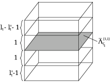
Figure 1:

Lemma 3.4

Let the function $V$ satisfy (4) and (5). Then with the notation above, we have for some $C>0$ and for $a_{1}\geq l_{1}+2$

$$-\log(Z_{\bar{\Lambda}^{a,l}}^{{{\psi}}_{u}}[\xi]) \leq -\log\bigl{(}Z_{\bar{\Lambda}^{a,l}_{[a_{1},l_{1}^{\prime}-1]}}^{{{\psi}}_{u}}[\xi]\bigr{)}-\log\bigl{(}Z_{\bar{\Lambda}^{a,l}_{[l_{1}^{\prime}+1,l_{1}]}}^{{{\psi}}_{u}}[\xi]\bigr{)}$$

$${}-\prod_{i=2}^{d}(l_{i}-a_{i}+1)\Biggl{(}\log C-\sum_{i=2}^{d}V(u_{i})\Biggr{)}$$

$${}-\sum_{x\in\bar{\Lambda}^{a,l}_{l_{1}^{\prime}}}u\cdot(l_{1}^{\prime},x_{2},\ldots,x_{d})\xi(x).\vspace*{-3pt}$$

We label the points $x\in\Lambda_{\bar{\Lambda}^{a,l}_{l_{1}^{\prime}}}$ as odd or even, depending on whether $\sum_{i=1}^{d}x_{i}$ is an odd or an even number. We will bound $Z^{{{{\psi}}_{u}}}_{\bar{\Lambda}^{a,l}}[\xi]$ from below by a product of $Z^{{{{\psi}}_{u}}}_{\bar{\Lambda}^{a,l}_{[a_{1},l_{1}^{\prime}-1]}}[\xi]$, of $Z^{{{{\psi}}_{u}}}_{\bar{\Lambda}^{a,l}_{[l_{1}^{\prime}+1,l_{1}]}}[\xi]$ and of terms coming from integrating out the contribution of the elements of $\bar{\Lambda}^{a,l}_{l_{1}^{\prime}}$ in $H_{\bar{\Lambda}^{a,l}}^{\psi_{u}}[\xi](\varphi).$ To do this, we will first integrate out the height variables at the odd points in $\bar{\Lambda}^{a,l}_{l_{1}^{\prime}}$ from $Z^{{{{\psi}}_{u}}}_{\bar{\Lambda}^{a,l}}[\xi]$ and then the even ones. We will do this by means of Lemma 3.3 and by splitting $H_{\bar{\Lambda}^{a,l}}^{\psi_{u}}[\xi](\varphi)$ into sums of potentials $V(\varphi(x)-\varphi(y))$, depending on whether $x$ and $y$ belong to $\bar{\Lambda}^{a,l}_{[a_{1},l_{1}^{\prime}-1]}$, $\bar{\Lambda}^{a,l}_{[l_{1}^{\prime}+1,l_{1}]}$, $\bar{\Lambda}^{a,l}_{l_{1}^{\prime}}$ or $\partial\bar{\Lambda}^{a,l}$. Then by Lemma 3.3, for each height variable $\varphi(x)$, $x\in\bar{\Lambda}^{a,l}_{l_{1}^{\prime}}$ with $x$ odd, (3.3) holds with $\gamma=u\cdot(l_{1}^{\prime},x_{2},\ldots,x_{d})$ (we recall that the boundary conditions for the two subdomains have the same tilt $u$ as for the original domain). Explicitly, for each height variable $\varphi(x)$, $x\in\Lambda_{\bar{\Lambda}^{a,l}_{l_{1}^{\prime}}}$ with $x$ odd, we have

$$\int_{\mathbb{R}}\exp\biggl{[}-\frac{1}{2}\sum_{j\in I}V\bigl{(}\varphi(x+e_{j})-\varphi(x)\bigr{)}+\xi(x)\varphi(x)\biggr{]}\,\mathrm{d}\varphi(x)$$

(43)

$$\qquad\geq C\exp\biggl{[}-\frac{1}{2}\sum_{j\in I}V\bigl{(}\varphi(x+e_{j})-x\cdot u\bigr{)}+\xi(x)(x\cdot u)\biggr{]},$$

where $I:=\{\pm 1,\pm 2,\ldots,\pm d\}$. The point here is that Lemma 3.3 allows us to replace a height variable $\varphi(x)$ by a deterministic value $\gamma$. Next we repeat the same procedure for each height variable $\varphi(x)$, $x\in\Lambda_{\bar{\Lambda}^{a,l}_{l_{1}^{\prime}}}$ and $x$ even; since all $\varphi(x+e_{j})$, with $x+e_{j}\in\Lambda_{\bar{\Lambda}^{a,l}_{l_{1}^{\prime}}}$ odd nearest neighbors of $x$, have already been integrated out by (3.1.2), we have

$$\int_{\mathbb{R}}\exp\biggl{[}-\frac{1}{2}\mathop{\sum_{j\in I}}_{j\neq\pm 1}V\bigl{(}(x+e_{j})\cdot u-\varphi(x)\bigr{)}-V\bigl{(}\varphi(x+e_{1})-\varphi(x)\bigr{)}$$

$$\hskip 116.0pt{}-V\bigl{(}\varphi(x+e_{-1})-\varphi(x)\bigr{)}+\xi(x)\varphi(x)\biggr{]}\,\mathrm{d}\varphi(x)$$

(44)

$$\qquad\geq C\exp\Biggl{[}-\frac{1}{2}V\bigl{(}\varphi(x+e_{1})-x\cdot u\bigr{)}-\frac{1}{2}V\bigl{(}\varphi(x-e_{1})-x\cdot u\bigr{)}$$

$$\hskip 177.0pt{}-\sum_{i=2}^{d}V(u_{i})+\xi(x)(x\cdot u)\Biggr{]}.$$

From (3.1.2) and (3.1.2) we get

$$Z^{{{{\psi}}_{u}}}_{\bar{\Lambda}^{a,l}}[\xi] \geq Z^{{{{\psi}}_{u}}}_{\bar{\Lambda}^{a,l}_{[a_{1},l_{1}^{\prime}-1]}}[\xi]Z^{{{{\psi}}_{u}}}_{\bar{\Lambda}^{a,l}_{[l_{1}^{\prime}+1,l_{1}]}}[\xi]$$

$${}\times\exp\Biggl{(}|\bar{\Lambda}^{a,l}_{l_{1}^{\prime}}|\log C-|\bar{\Lambda}^{a,l}_{l_{1}^{\prime}}|\sum_{i=2}^{d}V(u_{i})+\sum_{x\in{\bar{\Lambda}^{a,l}_{l_{1}^{\prime}}}}\xi(x)(x\cdot u)\Biggr{)}.$$

Plugging $|\bar{\Lambda}^{a,l}_{l_{1}^{\prime}}|=\prod_{i=2}^{d}(l_{i}-a_{i}+1)$ in the above, we get (3.4).

Proof of Theorem 1.10 We will use Lemma 3.4 together with Proposition 2.5 to prove in part (a1) below that $\lim_{N\rightarrow\infty}\sigma_{\Lambda_{N}}[\xi](u)$ exists for $\mathbb{P}$-almost all $\xi$ and Lemma 3.4 and Proposition 2.6 to derive in part (a2) the $L^{1}$ convergence. We will then use the a.s. and $L^{1}$ convergence in order to show in part (b) that the surface tension is independent of the disorder $(\xi(x))_{x\in\mathbb{Z}^{d}}$.

[(a1)]

We first need to rewrite (3.4) in Lemma 3.4 in a form such that we can apply Proposition 2.5. Let $a,l\in\mathbb{Z}^{d},a=(a_{i})_{1\leq i\leq d},l=(l_{i})_{1\leq i\leq d}$, with $a_{i}<l_{i}$ for $1\leq i\leq d$, be arbitrary and let, with the notation from Lemma 3.4,

$$g_{\bar{\Lambda}^{a,l}}:=\prod_{i=1}^{d}(l_{i}-a_{i}+1)\Biggl{(}\log C-\sum_{i=1}^{d}\frac{V(u_{i})}{2}\Biggr{)}.$$

Let $l+1=(l_{i}+1)_{1\leq i\leq d}$ and define $\bar{\Lambda}^{a,l+1}$ as in (23). Let

$$f_{\bar{\Lambda}^{a,l+1}}[\xi](u):=-\log(Z_{\bar{\Lambda}^{a,l}}^{\psi_{u}}[\xi])+\sum_{x\in\bar{\Lambda}^{a,l}}(u\cdot x)\xi(x)+g_{\bar{\Lambda}^{a,l}}.$$

Then from (3.4) we have the following subadditivity formula for $l_{1}\geq a_{1}+2$:

$$f_{\bar{\Lambda}^{a,l+1}}[\xi](u)\leq f_{\bar{\Lambda}^{a,l+1}_{[a_{1},l_{1}^{\prime}]}}[\xi](u)+f_{\bar{\Lambda}^{a,l+1}_{[l_{1}^{\prime}+1,l_{1}+1]}}[\xi](u).$$ (45)

To get the subadditivity formula (45) for all $l_{1}>a_{1}$, we use an argument similar to the one we used to obtain (3.1.1), to bound for $l_{1}\in\{a_{1},a_{1}+1\}$:

$$-\log Z_{\bar{\Lambda}^{a,l}_{[a_{1},l_{1}]}}^{\psi_{u}}[\xi] \leq \prod_{i=2}^{d}(l_{i}-a_{i}+1)\bigl{(}2dV(0)+\sigma^{C_{2}/2}[\xi=0](u=0)\bigr{)}$$

$${}-\sum_{x\in\bar{\Lambda}^{a,l}_{[a_{1},l_{1}]}}(u\cdot x)\xi(x)-\bigl{\langle}\xi,G_{\bar{\Lambda}^{a,l}_{[a_{1},l_{1}]}}\xi\bigr{\rangle}_{\bar{\Lambda}^{a,l}_{[a_{1},l_{1}]}},$$

where $\sigma^{C_{2}/2}[\xi=0](u=0)$ is defined as in Theorem 3.1(b). Taking into account that for all $\Lambda\in\mathbb{Z}^{d}$, $\langle\xi,G_{\Lambda}\xi\rangle_{\Lambda}\geq 0$, and making the convention that for all $a_{1}\in\mathbb{Z}$

$$f_{\Lambda_{\bar{\Lambda}^{a,l}_{[a_{1},a_{1}+1]}}}[\xi](u): = \prod_{i=2}^{2}(l_{i}-a_{i}+1)\bigl{(}2dV(0)+|\sigma^{C_{2}/2}[\xi=0](u=0)|\bigr{)}$$

$${}-\sum_{x\in\bar{\Lambda}^{a,l}_{[a_{1},a_{1}+1]}}(u\cdot x)\xi(x)+\bigl{\langle}\xi,G_{\bar{\Lambda}^{a,l}_{[a_{1},a_{1}+1]}}\xi\bigr{\rangle}_{\bar{\Lambda}^{a,l}_{[a_{1},a_{1}+1]}},$$

it follows that for all $l_{i}>a_{i},i=1,2,\ldots,d$, $f_{\bar{\Lambda}^{a,l+1}}[\xi](u)$ satisfies the subadditivity property (45) as defined in Proposition 2.5(b). We will check next that $f_{\bar{\Lambda}^{a,l+1}}[\xi](u)$ satisfies conditions (a) and (c) of Proposition 2.5. Recall that for $z\in{\mathbb{Z}^{d}}$, $\tau_{z}\varphi(x)=\varphi(x-z)\mbox{for}x\in{\mathbb{Z}^{d}}\mbox{and}\varphi\in\mathbb{R}^{{\mathbb{Z}^{d}}}$. As $(\xi(x))_{x\in{\mathbb{Z}^{d}}}$ are i.i.d., it is easy to see that condition (a) of Proposition 2.5 is satisfied. We will show next that (c) from Proposition 2.5 also holds. Using the lower bound in (3.1.1) and the fact that $\mathbb{E}(\xi(0))=0$, we have that $f_{\bar{\Lambda}^{a,l+1}}[\xi](u)\in L^{1}$. Moreover, by the same reasoning as that used to get (3.1.1), we have

$$\frac{\mathbb{E}(f_{\bar{\Lambda}^{a,l+1}}[\xi](u))}{|\bar{\Lambda}^{a,l}|}>\sigma^{A}[\xi=0](u=0)-\frac{\mathbb{E}(\xi^{2}(0))\sum_{x\in\bar{\Lambda}^{a,l}}G_{\bar{\Lambda}^{a,l}}(x,x)}{\bar{\Lambda}^{a,l}}-2dB.$$

Since by Proposition 2.1 we have that $\lim_{\Lambda\in\mathbb{Z}^{d},|\Lambda|\uparrow\infty}G_{\Lambda}(x,x)=G(0,0)<\infty$, it follows that

$$\mathop{\inf_{a,l\in\mathbb{Z}^{d},a_{i}<l_{i}}}_{i=1,\ldots,d}\frac{\mathbb{E}(f_{\bar{\Lambda}^{a,l}}[\xi](u))}{|\bar{\Lambda}^{a,l}|}>-\infty$$ (46)

and thus condition (c) of Proposition 2.5 is also satisfied. It follows that

$$\lim_{N\rightarrow\infty}\frac{f_{\Lambda_{N}[\xi](u)}}{N^{d}}\mbox{ exists a.s.}$$ (47)

Together with (3.1.1) this proves that $\lim_{N\rightarrow\infty}\sigma_{\Lambda_{N}}[\xi](u)$ exists for $\mathbb{P}$-almost all $\xi$.

To prove that $\lim_{N\rightarrow\infty}\sigma_{\Lambda_{N}}[\xi](u)$ exists in $L^{1}$, we will show that $f_{\bar{\Lambda}^{a,l+1}}[\xi](u)$ satisfies the assumptions of Proposition 2.6. Note first that assumption (a) is automatically satisfied, due to the subadditivity property derived in (45). Similarly, assumption (d) is satisfied because of (46). We will next prove that (b), (c) and (e) from Proposition 2.6 also hold. Let $z\in\mathbb{Z}^{d}$ and denote by $(\tilde{\psi})_{u}^{z}(x):=\sum_{i=1}^{d}(x_{i}u_{i}+z_{i})$ for $x\in\partial(\bar{\Lambda}^{a,l}+z)$. Then

$$\qquad f_{\bar{\Lambda}^{a,l+1}+z}[\xi](u) = -\log\bigl{(}Z_{\bar{\Lambda}^{a,l}+z}^{(\tilde{\psi})_{u}^{z}}[\xi]\bigr{)}+\sum_{x\in\bar{\Lambda}^{a,l}+z}(u\cdot x)\xi(x)+g_{\bar{\Lambda}^{a,l}+z}$$ (48)

$$= -\log(Z_{\bar{\Lambda}^{a,l}+z}^{\psi_{u}}[\xi])+\sum_{x\in\bar{\Lambda}^{a,l}}(u\cdot x)\xi(x+z)+g_{\bar{\Lambda}^{a,l}},$$ (49)

where in the first equality we made in the integral formula for $Z_{\bar{\Lambda}^{a,l}+z}^{(\tilde{\psi})_{u}^{z}}[\xi]$ the change of variables ${\hat{\varphi}}(x):=\varphi(x)+\sum_{i=1}^{d}z_{i}u_{i}$ for all $x\in\bar{\Lambda}^{a,l}+z$, and we used $g_{\bar{\Lambda}^{a,l}+z}=g_{\bar{\Lambda}^{a,l}}$. Since $(\xi(x))_{x\in\mathbb{Z}^{d}}$ are i.i.d., (48) proves that (b), (c) and (e) from Proposition 2.6 hold. It follows that all assumptions of Proposition 2.6 are satisfied. Therefore

$$\frac{f_{\Lambda_{N}}[\xi](u)}{N^{d}}\mbox{ converges in }L^{1}.$$

Together with (3.1.1) this proves that $\lim_{N\rightarrow\infty}\sigma_{\Lambda_{N}}[\xi](u)$ exists in $L^{1}$.

Since we were unable to find in the literature a result for multiparameter subadditive processes which we can apply directly as in (a1) and (a2) to show that $\sigma(u)[\xi]$ is independent of the disorder $\xi$, we will briefly sketch next a proof of the statement for our case. For simplicity of notation, we restrict ourselves to proving (b) for $\Lambda_{[0,N]}$, where we recall that $\Lambda_{[0,N]}=[0,N]^{d}\cap\mathbb{Z}^{d}$.

Let $k,n,r\in\mathbb{Z}_{+}$ such that $r<n$ and such that $N=kn+r$. For $a=(a_{i})_{1\leq i\leq d}\in\mathbb{Z}^{d}$, let $I_{a,n}:=\Lambda_{[(a_{1}-1)n,a_{1}n]\times\cdots\times[(a_{d}-1)n,a_{d}n]}$ and let $J_{N,k,n}^{s}:=\{z\in\mathbb{Z}^{d}\dvtx kn\leq z_{s}\leq N,0\leq z_{i}\leq N\mbox{ for }i=\{1,2,\ldots,d\}\setminus\{s\}\}$, where $s=1,2,\ldots,d$. Then

$$\Lambda_{[0,N]}=\bigcup_{\{1\leq a_{i}\leq k,i=1,\ldots d\}}I_{a,n}\cup\bigcup_{\{1\leq s\leq d\}}J_{N,k,n}^{s}.$$

In words, we are partitioning $\Lambda_{[0,N]}$ into the union of cubes of side lengths $n$, which are the $I$’s, and the $J$’s represent the leftover boundary terms because $N$ may not be divisible by $n$. Thus written, $\Lambda_{[0,N]}$ is a union of disjoint sets. From repeated application of (45), we have

$$f_{\Lambda_{[0,N]}}[\xi](u)\leq\sum_{\{1\leq a_{i}\leq k,i=1,\ldots,d\}}f_{I_{a,n}}[\xi](u)+\sum_{s=1}^{d}f_{J_{N,k,n}^{s}}[\xi](u).$$ (50)

The key of the proof is that we can use the ergodic theorem for the first sum in the right-hand side in (50) and that the boundary terms coming from the $J$’s are negligible. Combining this with the a.s. and the $L^{1}$ convergence of $N^{-d}f_{\Lambda_{[0,N]}}[\xi](u)$ proved in (a1) and (a2), the proof follows now similar steps to the proof of Theorem 1.10 from liggett and will be omitted.  ∎

3.2 Existence of shift-covariant random gradient Gibbs measures with given tilt

This subsection is structured as follows: in Section 3.2 we construct in (56) a sequence of spatially averaged finite-volume gradient Gibbs measures $(\bar{\mu}^{u}_{\Lambda}[\xi])_{\Lambda\subset\mathbb{Z}^{d}}$, such that $(\int\mathbb{P}(\mathrm{d}\xi)\bar{\mu}^{u}_{\Lambda}[\xi])_{\Lambda\subset\mathbb{Z}^{d}}$ is tight, as shown in Proposition 3.6, and shift-invariant. In Section 3.2.2 we will use the tightness of $(\int\mathbb{P}(\mathrm{d}\xi)\bar{\mu}^{u}_{\Lambda}[\xi])_{\Lambda\subset\mathbb{Z}^{d}}$ to prove in Theorem 1.7 the existence of a shift-covariant random gradient Gibbs measure with a given tilt $u\in\mathbb{R}^{d}$.

3.2.1 Tightness of the averaged measure

In order to prove tightness of the finite-volume gradient Gibbs measures averaged over the disorder, we look at the finite-volume Gibbs measures with tilt $u\in\mathbb{R}^{d}$ and boundary condition $\psi_{u}(x)=u\cdot x$:

$$\nu^{\psi_{u}}_{\Lambda}[\xi](\mathrm{d}\varphi) = \frac{1}{Z_{\Lambda}^{\psi_{u}}[\xi]}\exp\biggl{(}-\frac{1}{2}\mathop{\sum_{x,y\in\Lambda}}_{|x-y|=1}V\bigl{(}\varphi(x)-\varphi(y)\bigr{)}$$

$$\hskip 56.0pt{}-\mathop{\sum_{x\in\Lambda,y\in\partial\Lambda}}_{|x-y|=1}V\bigl{(}\varphi(x)-\psi_{u}(y)\bigr{)}$$

$$\hskip 117.0pt{}+\sum_{x\in\Lambda}\xi(x)\varphi(x)\biggr{)}\,\mathrm{d}\varphi_{\Lambda}\delta_{\psi_{u}}(\mathrm{d}\varphi_{\mathbb{Z}^{d}\setminus\Lambda}).$$

Let us look now at the quantity

$$\qquad F_{\beta,u,\Lambda}[\xi_{\Lambda}] := \log\int\nu^{\psi_{u}}_{\Lambda}[\xi](\mathrm{d}\varphi)$$

$${}\times\exp\biggl{(}+\frac{\beta}{2}\sum_{x,y\in{\mathbb{Z}^{d}},|x-y|=1}\bigl{(}\varphi(x)-\varphi(y)-u\cdot(x-y)\bigr{)}^{2}\biggr{)},$$

for $\beta>0$ sufficiently small. In (3.2.1), the sum over $x,y\in{\mathbb{Z}^{d}},|x-y|=1$, can be taken to include all the bonds on $\mathbb{Z}^{d}$ due to the fact that $\varphi=\psi_{u}$ on $\Lambda^{c}$. Note that $F_{\beta,u,\Lambda}$ is the difference between the original free energy in the volume $\Lambda$ and the free energy in the volume $\Lambda$ where we have added the term $\frac{\beta}{2}\sum_{x,y\in{\mathbb{Z}^{d}},|x-y|=1}(\varphi(x)-\varphi(y)-u\cdot(x-y))^{2}$ to the Hamiltonian.

We first note the following disorder-dependent upper bound for $F_{\beta,u,\Lambda}$.

Lemma 3.5

Let $d\geq 3$. Assume that $V$ satisfies (4) and (5). Then

$$F_{\beta,u,\Lambda}[\xi_{\Lambda}] \leq -|\Lambda|\bigl{(}\sigma_{\Lambda}^{A-\beta}[\xi=0](u=0)-\sigma_{\Lambda}^{C_{2}/2}[\xi=0](u=0)\bigr{)}$$

$${}+\mathop{\sum_{x,y\in\Lambda\cup\partial\Lambda}}_{|x-y|=1}\bigl{(}B+V(0)\bigr{)}$$

$${}-\frac{A-\beta-C_{2}/2}{2}\mathop{\sum_{x,y\in\Lambda\cup\partial\Lambda}}_{|x-y|=1}\bigl{(}(x-y)\cdot u\bigr{)}^{2}$$

$${}+\frac{1}{2}\biggl{(}\frac{1}{A-\beta}-\frac{2}{C_{2}}\biggr{)}\langle\xi,G_{\Lambda}\xi\rangle_{\Lambda}$$

$$=: \bar{F}_{\beta,u,\Lambda}+\frac{\alpha}{2}\langle\xi,G_{\Lambda}\xi\rangle_{\Lambda},$$

with the obvious definitions for $\bar{F}_{\beta,u,\Lambda}$ and $\alpha$.

Using bounds $As^{2}-B\leq V(s)\leq V(0)+\frac{C_{2}}{2}s^{2}$ for the potential $V$, we have

$$\exp(F_{\beta,u,\Lambda}[\xi_{\Lambda}])$$

$$\qquad\leq\int\exp\biggl{(}-\frac{1}{2}\mathop{\sum_{x,y\in\Lambda}}_{|x-y|=1}\bigl{(}A\bigl{(}\varphi(x)-\varphi(y)\bigr{)}^{2}-B\bigr{)}$$

$$\hskip 64.0pt{}-\mathop{\sum_{x\in\Lambda,y\in\partial\Lambda}}_{|x-y|=1}\bigl{(}A\bigl{(}\varphi(x)-\psi(y)\bigr{)}^{2}-B\bigr{)}+\sum_{x\in\Lambda}\xi(x)\varphi(x)\biggr{)}$$

$$\hskip 8.0pt\qquad\quad{}\times\exp\biggl{(}+\frac{\beta}{2}\sum_{x,y\in{\mathbb{Z}^{d}},|x-y|=1}\bigl{(}\varphi(x)-\varphi(y)-u\cdot(x-y)\bigr{)}^{2}\biggr{)}\,\mathrm{d}\varphi_{\Lambda}$$ (54)

$$\qquad\quad\Big{/}\int\exp\biggl{(}-\frac{1}{2}\mathop{\sum_{x,y\in\Lambda}}_{|x-y|=1}\biggl{(}\frac{C_{2}}{2}\bigl{(}\varphi(x)-\varphi(y)\bigr{)}^{2}+V(0)\biggr{)}$$

$$\hskip 78.0pt{}-\mathop{\sum_{x\in\Lambda,y\in\partial\Lambda}}_{\atop|x-y|=1}\biggl{(}\frac{C_{2}}{2}\bigl{(}\varphi(x)-\psi(y)\bigr{)}^{2}+V(0)\biggr{)}\biggr{)}$$

$$\qquad\hskip 22.0pt\quad{}\times\exp\biggl{(}\sum_{x\in\Lambda}\xi(x)\varphi(x)\biggr{)}\,\mathrm{d}\varphi_{\Lambda}.$$

This, by the same reasoning as in the proof of Theorem 3.1, is equal to

$$\int\exp\biggl{(}-\frac{1}{2}\mathop{\sum_{x,y\in\Lambda}}_{|x-y|=1}\bigl{(}(A-\beta)\bigl{(}\tilde{\varphi}(x)-\tilde{\varphi}(y)\bigr{)}^{2}$$

$$\qquad\hskip 62.0pt{}+(A-\beta)\bigl{(}(x-y)\cdot u\bigr{)}^{2}-B\bigr{)}$$

$$\hskip 11.0pt\qquad{}-\mathop{\sum_{x\in\Lambda,y\in\partial\Lambda}}_{|x-y|=1}\bigl{(}(A-\beta)(\tilde{\varphi}(x))^{2}+(A-\beta)\bigl{(}(x-y)\cdot u\bigr{)}^{2}-B\bigr{)}$$

$$\hskip 198.0pt\qquad{}+\sum_{x\in\Lambda}\xi(x)\tilde{\varphi}(x)\biggr{)}\,\mathrm{d}\tilde{\varphi}_{\Lambda}$$

(55)

$$\qquad{}\Big{/}\int\exp\biggl{(}-\frac{1}{2}\mathop{\sum_{x,y\in\Lambda}}_{|x-y|=1}\biggl{(}\frac{C_{2}}{2}\bigl{(}\tilde{\varphi}(x)-\tilde{\varphi}(y)\bigr{)}^{2}$$

$$\hskip 100.0pt\qquad{}+\frac{C_{2}}{2}\bigl{(}(x-y)\cdot u\bigr{)}^{2}+V(0)\biggr{)}$$

$$\hskip 42.0pt\qquad{}-\mathop{\sum_{x\in\Lambda,y\in\partial\Lambda}}_{|x-y|=1}\biggl{(}\frac{C_{2}}{2}(\tilde{\varphi}(x))^{2}+\frac{C_{2}}{2}\bigl{(}(x-y)\cdot u\bigr{)}^{2}+V(0)\biggr{)}$$

$$\hskip 207.0pt\qquad{}+\sum_{x\in\Lambda}\xi(x)\tilde{\varphi}(x)\biggr{)}\,\mathrm{d}\tilde{\varphi}_{\Lambda},$$

where we note the cancellation of a sum over $\xi$’s and where, as in the proof of Theorem 3.1, for all $x\in\Lambda$ we used the change of variables $\varphi(x)=\tilde{\varphi}(x)+x\cdot u$. The statement of the Lemma follows now by computing the Gaussian integrals above as in the proof of Theorem 3.1.

Take $\rho_{u}(b):=\nabla\psi_{u}(b)$ for all $b\in({\mathbb{Z}^{d}})^{*}$ and consider the corresponding gradient Gibbs measure $\mu_{\Lambda}^{\rho_{u}}[\xi]$ as given by (13). Let us now define the spatially averaged measure $\bar{\mu}^{u}_{\Lambda}[\xi]$ on gradient configurations obtained by

$$\bar{\mu}^{u}_{\Lambda}[\xi]:=\frac{1}{|\Lambda|}\sum_{x\in\Lambda}\mu^{\rho_{u}}_{\Lambda+x}[\xi],$$ (56)

where we recall that $\Lambda+x:=\{z+x\dvtx z\in\Lambda\}$. This is an extension to our disorder-dependent case of the construction on Gibbs measures with symmetries given in giorgii , in formula (5.20) from Chapter $5.2$; the construction in giorgii was used to get shift-invariant Gibbs measures. We note that in (56), the random field variables $\xi$ are held fixed while the volumes $\Lambda+x$ are shifted around. We will first use the fact that the measure $(\int\mathbb{P}(\mathrm{d}\xi)\bar{\mu}^{u}_{\Lambda}[\xi])(\mathrm{d}\varphi)$ is shift-invariant in the proof of Proposition 3.6 below. Then we will use $\bar{\mu}^{u}_{\Lambda}[\xi]$ to construct shift-covariant gradient Gibbs measures in Section 3.2.2 by performing a further average over the volumes.

In preparation for the proof of existence of random shift-covariant gradient Gibbs measures, we will prove the following result on the tightness of the family of averaged finite-volume random $\nabla\varphi$-Gibbs measures, and therefore on the existence, of the infinite-volume $\nabla\varphi$-Gibbs measures averaged over the disorder.

Proposition 3.6

Suppose that $d\geq 3$ and $\mathbb{E}(\xi(0))=0$. Assume that $V$ satisfies (4) and (5). Then there exists a constant $K>0$ such that for all $x_{0},y_{0}\in\mathbb{Z}^{d}$ with $|x_{0}-y_{0}|=1$, the measure

$$P^{u}_{\Lambda}(\mathrm{d}\varphi):=\biggl{(}\int\mathbb{P}(\mathrm{d}\xi)\bar{\mu}^{u}_{\Lambda}[\xi]\biggr{)}(\mathrm{d}\varphi)=\biggl{(}\frac{1}{|\Lambda|}\sum_{x\in\Lambda}\int\mathbb{P}(\mathrm{d}\xi)\mu^{\rho_{u}}_{\Lambda+x}[\xi]\biggr{)}(\mathrm{d}\varphi)$$

satisfies the estimate

$$\limsup_{N\uparrow\infty}P^{u}_{\Lambda_{N}}\bigl{[}\bigl{(}\varphi(x_{0})-\varphi(y_{0})-u\cdot(x_{0}-y_{0})\bigr{)}^{2}\bigr{]}\leq K.$$ (57)

Hence the sequence of measures $P^{u}_{\Lambda_{N}}$ is tight and thus possesses a disorder-independent limit measure (along subsequences of volumes) on gradient configurations.

Let $f\dvtx\mathbb{R}^{\mathbb{Z}^{d}}\rightarrow[0,\infty)$ be given by $f(\varphi):=(\varphi(x_{0})-\varphi(y_{0})-u\cdot(x_{0}-y_{0}))^{2}$; using translation invariance of the distribution of the disorder $(\xi(x))_{x\in\mathbb{Z}^{d}}$, we have

$$P^{u}_{\Lambda}(f) = \biggl{[}\frac{1}{|\Lambda|}\sum_{x\in\Lambda}\mathbb{E}\mu^{\rho_{u}}_{\Lambda+x}[\xi]\biggr{]}(f)=\frac{1}{|\Lambda|}\sum_{x\in\Lambda}(\mathbb{E}\mu^{\rho_{u}}_{\Lambda+x}[\xi])(f\circ\tau_{x})$$

$$= \frac{1}{|\Lambda|}\mathbb{E}\mu^{\rho_{u}}_{\Lambda}[\xi]\biggl{(}\sum_{x\in\Lambda}f\circ\tau_{x}\biggr{)}.$$

By the nonnegativity of $f$ we have for $\mathbb{P}$-almost all $\xi$

$$\mu^{\rho_{u}}_{\Lambda}[\xi]\biggl{(}\sum_{x\in\Lambda}f\circ\tau_{x}\biggr{)} \leq \mu^{\rho_{u}}_{\Lambda}[\xi]\biggl{(}\sum_{x,y\in{\mathbb{Z}^{d}},|x-y|=1}\bigl{(}\varphi(x)-\varphi(y)-u\cdot(x-y)\bigr{)}^{2}\biggr{)}$$

$$=: g[\xi].$$

By writing $g[\xi]=({2}/{\beta})\log e^{({\beta}/{2})g[\xi]}$ and applying Jensen’s inequality, we have

$$P^{u}_{\Lambda}(f) \leq \frac{1}{|\Lambda|}\mathbb{E}\mu^{\rho_{u}}_{\Lambda}[\xi]\biggl{(}\sum_{x,y\in{\mathbb{Z}^{d}},|x-y|=1}\bigl{(}\varphi(x)-\varphi(y)-u\cdot(x-y)\bigr{)}^{2}\biggr{)}$$

$$\leq \frac{2}{\beta|\Lambda|}\mathbb{E}\log\mu^{\rho_{u}}_{\Lambda}[\xi]\biggl{(}\exp\biggl{(}\frac{\beta}{2}\sum_{x,y\in{\mathbb{Z}^{d}},|x-y|=1}\bigl{(}\varphi(x)-\varphi(y)-u\cdot(x-y)\bigr{)}^{2}\biggr{)}\biggr{)}.$$

By Lemma 3.5 we get when $\Lambda=\Lambda_{N}$ the upper bound

$$P^{u}_{\Lambda_{N}}(f)\leq\frac{2}{\beta|\Lambda_{N}|}\bar{F}_{\beta,u,\Lambda_{N}}+\frac{2}{\beta|\Lambda_{N}|}\mathbb{E}\biggl{(}\frac{\alpha}{2}\langle\xi,G_{\Lambda_{N}}\xi\rangle_{\Lambda_{N}}\biggr{)},$$ (58)

which is bounded uniformly in $\Lambda_{N}$, as $\frac{\bar{F}_{\beta,u,\Lambda_{N}}}{|\Lambda_{N}|}$ is uniformly bounded by Theorem 1.10 and by (3.1.1), and $0\leq\frac{1}{|\Lambda_{N}|}\mathbb{E}(\langle\xi,G_{\Lambda_{N}}\xi\rangle_{\Lambda_{N}})\leq G(0,0)+1$, by Proposition 2.1(ii) and $\mathbb{E}(\xi(0))=0$. This proves the claim.

3.2.2 Existence of shift-covariant random gradient Gibbs measures with given tilt

In this subsection we will prove our main result, Theorem 1.7, of existence of a shift-covariant random gradient Gibbs measure $\hat{\mu}^{u}[\xi]$ with a given tilt $u\in\mathbb{R}^{d}$. In the proof, we will first construct a candidate $\hat{\mu}^{u}[\xi]$ by taking suitable subsequential weak limits, and then in two subsequent Lemmas 3.9 and 3.10, we will prove, respectively, that $\mathbb{P}$-a.s., our candidate $\hat{\mu}^{u}[\xi]$ is a gradient Gibbs measure, and is translation-covariant.

To construct a candidate $\hat{\mu}^{u}[\xi]$, we will need to perform a further average of $\bar{\mu}^{u}[\xi]$ over the volumes $\Lambda$, and to find a deterministic sequence $(m_{r})_{r\in\mathbb{N}}$, along which there is a weak limit for $\mathbb{P}$-a.e. $\xi$. This will be facilitated by Theorem 1a from KOM , which we state below.

Proposition 3.7

If $(\zeta_{n})_{n\in\mathbb{N}}$ is a sequence of real-valued random variables with $\lim\inf_{n\rightarrow\infty}\mathbb{E}(|\zeta_{n}|)<\infty$, then there exists a subsequence $\{\theta_{n}\}_{n\in\mathbb{N}}$ of the sequence $\{\zeta_{n}\}_{n\in\mathbb{N}}$ and an integrable random variable $\theta$ such that for any arbitrary subsequence $\{\tilde{\theta}_{n}\}_{n\in\mathbb{N}}$ of the sequence $\{\theta_{n}\}$, we have

$$\lim_{n\rightarrow\infty}\frac{\tilde{\theta}_{1}+\tilde{\theta}_{2}+\cdots+\tilde{\theta}_{n}}{n}=\theta\qquad\mathbb{P}\mbox{-almost surely}.$$

We are now ready to prove the existence of shift-covariant gradient Gibbs measures in Theorem 1.7, which follows immediately from the next Proposition.

Proposition 3.8

Suppose that $d\geq 3$ and $\mathbb{E}(\xi(0))=0$. Assume that $V$ satisfies (4) and (5). Then there is a deterministic sequence $(m_{r})_{r\in\mathbb{N}}$ in $\mathbb{N}$ such that for $\mathbb{P}$-almost every $\xi$,

$$\hat{\mu}^{u}_{k}[\xi]:=\frac{1}{k}\sum_{i=1}^{k}{\bar{\mu}}^{u}_{\Lambda_{m_{i}}}[\xi]$$ (59)

converges as $k\to\infty$ weakly to $\hat{\mu}^{u}[\xi]$, which is a shift-covariant random gradient Gibbs measure defined as in Definition 1.6.

We will prove first that there exists a deterministic sequence $(m_{r})_{r\in\mathbb{N}}$ in $\mathbb{N}$ such that $(\hat{\mu}^{u}_{k}[\xi])_{k\in\mathbb{N}}$ converges a.s. to a random measure $\hat{\mu}^{u}[\xi]$. We will then show that $\hat{\mu}^{u}[\xi]$ is a.s. a gradient Gibbs measure, is translation-covariant and that $\xi\rightarrow\hat{\mu}^{u}[\xi]$ is a measurable map.

Let $(f_{i})_{i\in\mathbb{N}}$ be a countable collection of functions in $C_{b}(\chi)$, such that a sequence of probability measures $\mu_{n}\in P(\chi)$ converges weakly to $\mu\in P(\chi)$ if and only if $\mu_{n}(f_{i})\to\mu(f_{i})$ for all $i\in\mathbb{N}$. Such a countable family $(f_{i})_{i\in\mathbb{N}}$ in $C_{b}(\chi)$ is explicitly given, for example, in the general setting of separable and complete metric spaces in Proposition 3.17 from RES or in Lemma 1.1 from Kal . To show that for a given sequence $(m_{r})_{r\in\mathbb{N}}$ and a random measure $\hat{\mu}[\xi]$, $\hat{\mu}_{k}[\xi]$ converges a.s. to $\hat{\mu}[\xi]$, it suffices to show that $\hat{\mu}_{k}[\xi](f_{i})\to\hat{\mu}[\xi](f_{i})$ almost surely for each $i\in\mathbb{N}$.

For each $N\in\mathbb{N}$ and $x,y\in\mathbb{Z}^{d}$ with $|x-y|=1$, define

$$X_{N;x,y}[\xi]:=\bar{\mu}_{\Lambda_{N}}^{u}[\xi]\bigl{(}\bigl{(}\varphi(x)-\varphi(y)-u\cdot(x-y)\bigr{)}^{2}\bigr{)}.$$ (60)

Take now the countable sequence containing both the family $(\bar{\mu}_{\Lambda_{N}}^{u}[\xi](f_{i}))_{i,N\in\mathbb{N}}$ and $(X_{N;x,y}[\xi])_{N\in\mathbb{N},x,y\in\mathbb{Z}^{d}\atop|x-y|=1}$. We note that since $(f_{i})_{i\in\mathbb{N}}$ are bounded functions, $\lim\inf_{N\uparrow\infty}\mathbb{E}(\bar{\mu}_{\Lambda_{N}}^{u}[\xi](|f_{i}|))<|f_{i}|_{\infty}<\infty$. Note also that $\liminf_{N}\mathbb{E}(X_{N;x,y}[\xi])<\infty$ by Proposition 3.6. Therefore by Proposition 3.7, for each $x_{0},y_{0}\in\mathbb{Z}^{d}$ with $|x_{0}-y_{0}|=1$, there exists a sequence $(n_{r})_{r\in\mathbb{N}}$ and a random variable $\kappa_{x_{0},y_{0}}$, both depending on $x_{0}$ and $y_{0}$, such that

$$\lim_{k\uparrow\infty}\frac{1}{k}\sum_{r=1}^{k}X_{n_{r};x_{0},y_{0}}[\xi]=\kappa_{x_{0},y_{0}}[\xi]\qquad\mbox{for }\mathbb{P}\mbox{-almost every }\xi.$$

Moreover

$$\lim_{k\uparrow\infty}\frac{1}{k}\sum_{j=1}^{k}X_{n_{r_{j}};x_{0},y_{0}}[\xi]=\kappa_{x_{0},y_{0}}[\xi]\qquad\mbox{for }\mathbb{P}\mbox{-almost every }\xi$$

holds also for every further subsequence $(n_{r_{j}})_{r_{j}\in\mathbb{N}}$ of $(n_{r})_{r\in\mathbb{N}}$. We take an arbitrary such subsequence $n_{r_{j}}$. By Proposition 3.7, there exists a subsequence $(n^{\prime}_{r})_{r\in\mathbb{N}}$ of $(n_{r_{j}})_{r_{j}\in\mathbb{N}}$ and a random variable $\rho_{1}$, both depending on $x_{0}$ and $y_{0}$, such that

$$\lim_{k\uparrow\infty}\frac{1}{k}\sum_{j=1}^{k}\bar{\mu}_{\Lambda_{n^{\prime}_{r_{j}}}}^{u}[\xi](f_{1})=\rho_{1}[\xi]\qquad\mbox{for }\mathbb{P}\mbox{-almost every }\xi.$$

Moreover

$$\lim_{k\uparrow\infty}\frac{1}{k}\sum_{j=1}^{k}\bar{\mu}_{\Lambda_{n^{\prime\prime}_{r_{j}}}}[\xi](f_{1})=\rho_{1}[\xi]\qquad\mbox{for }\mathbb{P}\mbox{-almost every }\xi$$

holds also for every further subsequence $n^{\prime\prime}_{r_{j}}$ of $n^{\prime}_{r_{j}}$.

We repeat this procedure for each $x,y\in\mathbb{Z}^{d},|x-y|=1$ and for each $i\in\mathbb{N}$. By a Cantor diagonalization argument over the countably many $x,y\in\mathbb{Z}^{d},|x-y|=1$ and over the $i\in\mathbb{N}$, there exists a deterministic sequence $(m_{r})_{r\in\mathbb{N}}$ in $\mathbb{N}$ and random variables $(\kappa_{x,y}[\xi])_{x,y\in\mathbb{Z}^{d},|x-y|=1}$ and $(\rho_{i}[\xi])_{i\in\mathbb{N}}$ such that for $\mathbb{P}$-almost every $\xi$,

$$\lim_{k\uparrow\infty}\frac{1}{k}\sum_{r=1}^{k}X_{m_{r};x,y}[\xi] = \kappa_{x,y}[\xi]\quad\mbox{and}$$

$$\lim_{k\uparrow\infty}\frac{1}{k}\sum_{r=1}^{k}\bar{\mu}_{\Lambda_{m_{r}}}^{u}[\xi](f_{i}) = \rho_{i}[\xi],$$

for all $x,y\in\mathbb{Z}^{d}$ and all $i\in\mathbb{N}$. In particular, we get from (3.2.2) that$\sup_{k\in\mathbb{N}}{\hat{X}}_{k;x,y}[\xi]\leq C(\kappa_{x,y}[\xi])$ for some $C(\kappa_{x,y}[\xi])>0$. Therefore for all $b\in(\mathbb{Z}^{d})^{*}$, with $b=(x,y)$, we have for $\mathbb{P}$-almost every $\xi$

$$\lim_{L\uparrow\infty}\sup_{k\in\mathbb{N}}{\hat{\mu}}_{k}^{u}[\xi]\bigl{(}\eta\dvtx|\eta(b)|\geq L\bigr{)}\leq\lim_{L\uparrow\infty}\sup_{k\in\mathbb{N}}\frac{{\hat{X}}_{k;x,y}[\xi]}{L^{2}}=0.$$

This means that for $\mathbb{P}$-a.s. all $\xi$, there exists a (possibly) random subsequence $(k^{\prime}[\xi])$ such that $({\hat{\mu}}_{k^{\prime}[\xi]}^{u}[\xi])_{k^{\prime}[\xi]}$ is tight and converges weakly to a random measure $\hat{\mu}^{u}[\xi]$. The random subsequence $(k^{\prime}[\xi])$ is used only for tightness; in fact the subsequence becomes nonrandom again as we return below to the deterministic subsequence $(m_{r})$. Moreover, we have ${\hat{\mu}}_{k^{\prime}[\xi]}^{u}[\xi](f_{i})\rightarrow\hat{\mu}^{u}[\xi](f_{i})$ for all $i\in\mathbb{N}$. Due to (3.2.2), and by the uniqueness of the limit point, we get that $\rho_{i}[\xi]=\hat{\mu}^{u}[\xi](f_{i})$ for all $i\in I$. Since $\hat{\mu}_{k}^{u}[\xi](f_{i})\rightarrow\hat{\mu}^{u}[\xi](f_{i})$, it follows that $\hat{\mu}_{k}^{u}[\xi]$ converges a.s. to a random measure $\hat{\mu}^{u}[\xi]$.

From Lemma 3.9 below, we get that for $\mathbb{P}$-almost all $\xi$, $\hat{\mu}^{u}[\xi]$ is a gradient Gibbs measure and from Lemma 3.10 below, that $\hat{\mu}^{u}[\xi]$ is translation-covariant for $\mathbb{P}$-almost all $\xi$.

It only remains to prove that $\xi\rightarrow\hat{\mu}^{u}[\xi]$ is a measurable map. We recall that the disorder is defined on the probability space $(\Omega,\mathcal{F},\mathbb{P})$. With a given tilted boundary condition $\psi_{u}$, $\mu^{\psi_{u}}_{\Lambda}[\xi]$ is clearly a measurable function of the disorder field $\xi$. Since $\hat{\mu}^{u}$ is constructed as a pointwise (w.r.t. $\xi$) limit of averages of such measurable $\mathbb{P}(\chi)$-valued functions of $\xi$, $\hat{\mu}^{u}$ is also a measurable $\mathbb{P}(\chi)$-valued function of $\xi$.

We will prove next Lemmas 3.9 and 3.10. The setup is as before; that is, $\hat{\mu}^{u}_{k}[\xi]$ is defined as in (56), and the assumption is that along a deterministic subsequence $(m_{i})_{i\in\mathbb{N}}$ in $\mathbb{N}$, we have weak convergence of $\hat{\mu}^{u}_{k}[\xi]$ to $\hat{\mu}^{u}[\xi]$ for $\mathbb{P}$-almost all $\xi$.

Lemma 3.9

For $\mathbb{P}$-almost all $\xi$, the limit $\hat{\mu}^{u}[\xi]$ is a gradient Gibbs measure.

In order to show that $\hat{\mu}^{u}[\xi]$ is a gradient Gibbs measure, we have to show that for each fixed $\xi$, for all $F\in C_{b}(\chi)$ and for all $J\subset\mathbb{Z}^{d}$ we have

$$\int\hat{\mu}^{u}[\xi](\mathrm{d}\tilde{\rho})\int\mu_{J}^{\tilde{\rho}}[\xi](\mathrm{d}\eta)F(\eta)=\int\hat{\mu}^{u}[\xi](\mathrm{d}\eta)F(\eta).$$ (62)

Using the compatibility of the kernels, namely

$$\int\mu^{\rho_{u}}_{\Lambda}[\xi](\mathrm{d}\tilde{\rho})\mu^{\tilde{\rho}}_{J}[\xi]=\mu^{\rho_{u}}_{\Lambda}[\xi]\qquad\mbox{for }J\subset\Lambda\subset\mathbb{Z}^{d},$$

we have

$$\int\bar{\mu}^{u}_{\Lambda}[\xi](\mathrm{d}\tilde{\rho})\mu^{\tilde{\rho}}_{J}[\xi]$$

$$\qquad=\frac{1}{|\Lambda|}\sum_{x\in\Lambda}\int\mu^{\rho_{u}}_{\Lambda+x}[\xi](\mathrm{d}\tilde{\rho})\mu^{\tilde{\rho}}_{J}[\xi]$$

$$\qquad=\frac{1}{|\Lambda|}\biggl{(}\sum_{x\in\Lambda\dvtx J{\subset}\Lambda+x}+\sum_{x\in\Lambda\dvtx J\not{\subset}\Lambda+x}\biggr{)}\int\mu^{\rho_{u}}_{\Lambda+x}[\xi](\mathrm{d}\tilde{\rho})\mu^{\tilde{\rho}}_{J}[\xi]$$ (63)

$$\qquad=\frac{1}{|\Lambda|}\sum_{x\in\Lambda\dvtx J{\subset}\Lambda+x}\mu^{\rho_{u}}_{\Lambda+x}[\xi]+\frac{1}{|\Lambda|}\sum_{x\in\Lambda\dvtx J\not{\subset}\Lambda+x}\int\mu^{\rho_{u}}_{\Lambda+x}[\xi](\mathrm{d}\tilde{\rho})\mu^{\tilde{\rho}}_{J}[\xi]$$

$$\qquad=\bar{\mu}^{u}_{\Lambda}[\xi]+\frac{1}{|\Lambda|}\sum_{x\in\Lambda\dvtx J\not{\subset}\Lambda+x}\biggl{(}\int\mu^{\rho_{u}}_{\Lambda+x}[\xi](\mathrm{d}\tilde{\rho})\mu^{\tilde{\rho}}_{J}[\xi]-\mu^{\rho_{u}}_{\Lambda+x}[\xi]\biggr{)}.$$

Fix $J\subset\mathbb{Z}^{d}$ and take $k\in\mathbb{N}$ large enough. Applying (3.2.2) to the subsequence $(\Lambda_{m_{i}})_{1\leq m_{i}\leq k}$ and to an arbitrary $F\in C_{b}(\chi)$, we have

$$\quad\hat{\mu}^{u}_{k}[\xi](\mu^{\tilde{\rho}}_{J}[\xi](F))=\frac{1}{k}\sum_{i=1}^{k}\bar{\mu}^{u}_{\Lambda_{m_{i}}}[\xi](F)+\frac{1}{k}\sum_{i=1}^{k}R(\Lambda_{m_{i}},J,F)[\xi],$$ (64)

where $|R(\Lambda_{m_{i}},J,f)[\xi]|\leq\frac{C(f)}{|\Lambda_{m_{i}}|}\sum_{x\in\Lambda_{m_{i}}\dvtx J\not{\subset}\Lambda_{m_{i}}+x}1$, for all $1\leq i\leq k$ and for some constant $C(f)>0$. In order to prove (62), we need to take $k\rightarrow\infty$ on both sides of (64). To do that, we have to prove first that for all $F\in C_{b}(\chi)$ and for all fixed $J\subset\mathbb{Z}^{d}$ we have

$$\int\hat{\mu}[\xi](\mathrm{d}\tilde{\rho})(\mu^{\tilde{\rho}}_{J}[\xi](F))=\lim_{k\uparrow\infty}\hat{\mu}^{u}_{k}[\xi](\mu^{\tilde{\rho}}_{J}[\xi](F)).$$ (65)

To show (65), it is sufficient to show that for all $F\in C_{b}(\chi)$ the function $\mu^{\tilde{\rho}}_{J}[\xi](F)\in C_{b}(\chi)$ as a function in $\tilde{\rho}$; then (65) will follow by the hypothesis. The boundedness of $\mu^{\tilde{\rho}}_{J}[\xi](F)$ follows immediately due to the boundedness of $F$. To prove continuity of $\mu^{\tilde{\rho}}_{J}[\xi](F)$, fix $\tilde{\rho}\in\chi$ arbitrarily. As $\chi$ equipped with the metric $\|_{r}$ is a complete metric space, we can take now a sequence $({\tilde{\rho}}_{n})_{n\in\mathbb{N}}\in\chi$ such that $\lim_{n\uparrow\infty}{\tilde{\rho}}_{n}=\tilde{\rho}$ in $\chi$; we have to show that $\lim_{n\uparrow\infty}\mu^{{\tilde{\rho}}_{n}}_{J}[\xi](F)=\mu^{\tilde{\rho}}_{J}[\xi](F)$. In view of the fact that $V\in C^{2}(\mathbb{R})$, we note now that both the integrand in the numerator, and the integrand in the denominator, of $\lim_{n\uparrow\infty}\mu^{{\tilde{\rho}}_{n}}_{J}[\xi](F)$ converge as ${\tilde{\rho}}_{n}\rightarrow{\tilde{\rho}}$; moreover, due to the bounds $As^{2}-B\leq V(s)\leq V(0)+\frac{C_{2}}{2}s^{2}$ on the potential $V$ and by a similar reasoning as in the proof of Lemma 3.5, these integrands are uniformly bounded by integrable functions. Applying now Lebesgue’s dominated convergence theorem separately to the numerator and to the denominator gives $\lim_{n\uparrow\infty}\mu^{{\tilde{\rho}}_{n}}_{J}[\xi](F)=\mu^{\tilde{\rho}}_{J}[\xi](F)$, and therefore (65) holds. Taking $k$ to infinity in (64) and using (65), we get

$$\int\hat{\mu}[\xi](\mathrm{d}\tilde{\rho})(\mu^{\tilde{\rho}}_{J}[\xi](F)) = \lim_{k\uparrow\infty}\frac{1}{k}\sum_{i=1}^{k}\bar{\mu}^{u}_{\Lambda_{m_{i}}}[\xi](F)+\lim_{k\uparrow\infty}\frac{1}{k}\sum_{i=1}^{k}R(\Lambda_{m_{i}},J,F)[\xi]$$

$$= \hat{\mu}^{u}[\xi](F)+0,$$

where the convergence holds due to the fact that $F\in C_{b}(R^{({\mathbb{Z}^{d}})^{*}})$ and$\sum_{i=1}^{k}R(\Lambda_{m_{i}},J,F)[\xi]/k$ goes to zero uniformly in $\xi$, due to the upper bound on $|R(\Lambda,J,F)[\xi]|$. This proves that (62) holds.

Lemma 3.10

For $\mathbb{P}$-almost all $\xi$, the limit $\hat{\mu}^{u}[\xi]$ is translation-covariant, that is, for all $v\in\mathbb{Z}^{d}$ and for all $F\in C_{b}(\chi)$, we have

$$\hat{\mu}^{u}[\xi](F\circ\tau_{v})=\hat{\mu}^{u}[\tau_{v}\xi](F),$$ (66)

where we recall that $(\tau_{v}\xi)(z)=\xi(z-v)$ for all $z\in\mathbb{Z}^{d}$.

Fix $v\in\mathbb{Z}^{d}$. Then we have

$$\hat{\mu}^{u}[\xi](F\circ\tau_{v})-\hat{\mu}^{u}[\tau_{v}\xi](F)$$

$$\qquad=\lim_{k\uparrow\infty}\frac{1}{k}\sum_{i=1}^{k}\frac{1}{|\Lambda_{m_{i}}|}\biggl{(}\sum_{x\in\Lambda_{m_{i}}}\mu^{\rho_{u}}_{\Lambda_{m_{i}}+x}[\xi](F\circ\tau_{v})$$ (67)

$$\hskip 88.0pt\qquad{}-\sum_{x\in\Lambda_{m_{i}}}\mu^{\rho_{u}}_{\Lambda_{m_{i}}+x}[\tau_{v}\xi](F)\biggr{)}.$$

The terms inside the last bracket equal

$$\sum_{x\in\Lambda_{m_{i}}}\mu^{\rho_{u}}_{\Lambda_{m_{i}}+x}[\xi](F\circ\tau_{v})-\sum_{x\in\Lambda_{m_{i}}}\mu^{\rho_{u}}_{\Lambda_{m_{i}}+x}[\tau_{v}\xi](F)$$

$$\qquad=\sum_{x\in\Lambda_{m_{i}+v}}\mu^{\rho_{u}}_{\Lambda_{m_{i}}+x}[\xi](F)-\sum_{x\in\Lambda_{m_{i}}}\mu^{\rho_{u}}_{\Lambda_{m_{i}}+x}[\xi](F).$$

Most terms on the right-hand side cancel. Therefore, for a bounded function $F$ such that $\|F\|_{\infty}\leq C(F)$ for some $C(F)>0$, we have

$$|\hat{\mu}^{u}[\xi](F)-\hat{\mu}^{u}[\tau_{v}\xi](F)|\leq\lim_{k\uparrow\infty}\frac{C(F)}{k}\sum_{i=1}^{k}\frac{|{\Lambda}_{m_{i}}\triangle({\Lambda}_{m_{i}}+v)|}{|{\Lambda}_{m_{i}}|},$$ (68)

where we denoted by $\Delta$ the symmetric difference of the sets $\Lambda$ and $\Lambda+v$. But $|\Lambda_{m_{i}}\triangle(\Lambda_{m_{i}}+v)|$ goes to zero when divided by $|\Lambda_{m_{i}}|$, uniformly in $m_{i}$, which implies that (68) goes to zero also. This shows the translation-covariance.

Proof of Theorem 1.7(a) Proposition 3.8 implies the existence of a random gradient Gibbs $\hat{\mu}^{u}[\xi]$. We prove next that $\hat{\mu}^{u}[\xi]$ satisfies (1.7). Given the tilt $u\in\mathbb{R}^{d}$, the limit $\hat{\mu}^{u}[\xi]$ we construct is the weak limit of the $\hat{\mu}_{k}^{u}[\xi]$. We next calculate what is the expected tilt over a given bond under the measure $\hat{\mu}_{k}^{u}[\xi]$, averaged over the disorder. For any $m_{i}$ in the deterministic sequence $(m_{i})_{1\leq i\leq k}$ and for $b_{1}:=(0,e_{1})$, we have by means of (56) and of Definition (13)

$$\bar{\mu}_{m_{i}}^{\rho_{u}}[\xi](\eta(b_{1})) = \frac{1}{|\Lambda_{m_{i}}|}\sum_{x\in\Lambda_{m_{i}}}\mu^{\rho_{u}}_{\Lambda_{m_{i}}+x}[\xi](\eta(b_{1}))$$

$$= \frac{1}{|\Lambda_{m_{i}}|}\sum_{x\in\Lambda_{m_{i}}}\nu^{\psi_{u}}_{\Lambda_{m_{i}}+x}[\xi]\bigl{(}\varphi(e_{1})-\varphi(0)\bigr{)}$$

$$= \frac{1}{|\Lambda_{m_{i}}|}\sum_{x\in\Lambda_{m_{i}}}\nu^{\tau_{-x}\psi_{u}}_{\Lambda_{m_{i}}}[\tau_{-x}\xi]\bigl{(}\varphi(e_{1}-x)-\varphi(-x)\bigr{)}$$

$$= \frac{1}{|\Lambda_{m_{i}}|}\sum_{x\in\Lambda_{m_{i}}}\nu^{\psi_{u}}_{\Lambda_{m_{i}}}[\tau_{-x}\xi]\bigl{(}\varphi(e_{1}-x)-\varphi(-x)\bigr{)},$$

where for the third equality we made for all $y\in\Lambda_{m_{i}}$ the change of variables $\varphi(y)\rightarrow\varphi(y)+\sum_{i=1}^{d}u_{i}x_{i}$ under each integral. Let

$$\bar{\Lambda}^{-m_{i},m_{i}}_{m_{i}} := \Lambda_{\{m_{i}\}\times[-m_{i},m_{i}]\times\cdots\times[-m_{i},m_{i}]}\quad\mbox{and}$$

$$\bar{\Lambda}^{-m_{i},m_{i}}_{-m_{i}} := \Lambda_{\{-m_{i}\}\times[-m_{i},m_{i}]\times\cdots\times[-m_{i},m_{i}]}.$$

Averaging over the disorder in (3.2.2), we get

$$\mathbb{E}\biggl{(}\int\bar{\mu}_{m_{i}}^{\rho_{u}}[\xi](\mathrm{d}\eta)\eta(b_{1})\biggr{)}$$

$$\qquad=\frac{1}{|\Lambda_{m_{i}}|}\sum_{x\in\Lambda_{m_{i}}}\mathbb{E}\biggl{(}\int\nu^{\psi_{u}}_{\Lambda_{m_{i}}}[\tau_{-x}\xi](\mathrm{d}\varphi)\bigl{(}\varphi(e_{1}-x)-\varphi(-x)\bigr{)}\biggr{)}$$

$$\qquad=\frac{1}{|\Lambda_{m_{i}}|}\sum_{x\in\Lambda_{m_{i}}}\mathbb{E}\biggl{(}\int\nu^{\psi_{u}}_{\Lambda_{m_{i}}}[\xi](\mathrm{d}\varphi)\bigl{(}\varphi(e_{1}-x)-\varphi(-x)\bigr{)}\biggr{)}$$

$$\qquad=\frac{1}{|\Lambda_{m_{i}}|}\sum_{x\in\{\Lambda_{m_{i}}\setminus\bar{\Lambda}^{-m_{i},m_{i}}_{-m_{i}}\}}\mathbb{E}\biggl{(}\int\nu^{\psi_{u}}_{\Lambda_{m_{i}}}[\xi](\mathrm{d}\varphi)\bigl{(}\varphi(e_{1}-x)-\varphi(-x)\bigr{)}\biggr{)}$$

$$\quad\qquad{}+\frac{1}{|\Lambda_{m_{i}}|}\sum_{x\in\bar{\Lambda}^{-m_{i},m_{i}}_{-m_{i}}}\mathbb{E}\biggl{(}\int\nu^{\psi_{u}}_{\Lambda_{m_{i}}}[\xi](\mathrm{d}\varphi)\bigl{(}\psi(e_{1}-x)-\varphi(-x)\bigr{)}\biggr{)}.$$

Most of the terms in the last equality in the above equation cancel and we are left with

$$\mathbb{E}\biggl{(}\int\bar{\mu}_{m_{i}}^{\rho_{u}}[\xi](\mathrm{d}\eta)\eta(b_{1})\biggr{)}$$

$$\qquad=\frac{1}{|\Lambda_{m_{i}}|}\biggl{[}\sum_{x\in\bar{\Lambda}^{-m_{i},m_{i}}_{-m_{i}}}\psi(e_{1}-x)-\sum_{x\in\bar{\Lambda}^{-m_{i},m_{i}}_{m_{i}}}\bigl{(}u_{1}+\psi(-e_{1}-x)\bigr{)}$$

$$\hskip 63.0pt{}-\sum_{x\in\bar{\Lambda}^{-m_{i},m_{i}}_{m_{i}}}\mathbb{E}\biggl{(}\int\nu^{\psi_{u}}_{\Lambda_{m_{i}}}[\xi](\mathrm{d}\varphi)\bigl{(}\varphi(-x)-\psi(-e_{1}-x)-u_{1}\bigr{)}\biggr{)}\biggr{]}$$

$$\qquad=u_{1}+\frac{O(K,u_{1})}{2m_{i}+1},$$

uniformly in $m_{i}\in\mathbb{N}$, and where to bound the last term in the first equality, we used Proposition 3.6. From this, it follows easily that we have, uniformly in $k\in\mathbb{N}$,

$$\mathbb{E}\biggl{(}\int\hat{\mu}_{k}^{u}[\xi](\mathrm{d}\eta)\eta(b_{1})\biggr{)}=u_{1}+\frac{o(\log k)}{k}.$$

Fix any large $M>0$. Then $\eta(b)\wedge M\vee(-M)$ is bounded and continuous, so for $\mathbb{P}$-a.s. all $\xi$, we have

$$\lim_{k\rightarrow\infty}\int\hat{\mu}_{k}^{u}[\xi](\mathrm{d}\eta)\eta(b)\wedge M\vee(-M)=\int\hat{\mu}^{u}[\xi](\mathrm{d}\eta)\eta(b)\wedge M\vee(-M).$$

Moreover, from Proposition 3.6 and Chebyshev’s inequality, we have

$$\mathbb{E}\biggl{(}\int\hat{\mu}_{k}^{u}[\xi](\mathrm{d}\eta)\eta(b)\biggr{)}=\mathbb{E}\biggl{(}\int\hat{\mu}_{k}^{u}[\xi](\mathrm{d}\eta)\eta(b)\wedge M\vee(-M)\biggr{)}+\frac{O(K)}{M^{d}},$$

uniformly in $k\in\mathbb{N}$. Therefore by sending $M$ to $\infty$, the convergence of the truncated $\eta$ together with the fact that $\int\hat{\mu}^{u}[\xi](\mathrm{d}\eta)\eta(b)$ is an integrable random variable, proves (1.7). By symmetry, (1.7) holds for any $b\in({\mathbb{Z}^{d}})^{*}$.

To prove (19), take any $b=(x_{0},y_{0})\in(\mathbb{Z}^{d})^{*}$. Since $(\varphi(x_{0})-\varphi(y_{0})-u\cdot(x_{0}-y_{0}))^{2}\geq 0$, by the weak convergence of $({\hat{\mu}}_{k}^{u})_{k\in\mathbb{N}}$ to ${\hat{\mu}}^{u}$ and by Proposition 3.6, we have

$$\mathbb{E}\biggl{(}\int{\hat{\mu}^{u}}[\xi](\mathrm{d}\eta)\bigl{(}\varphi(x_{0})-\varphi(y_{0})-u\cdot(x_{0}-y_{0})\bigr{)}^{2}\biggr{)}$$

(70)

$$\qquad\leq\mathbb{E}\Bigl{(}\lim\inf_{k\rightarrow\infty}{\hat{\mu}}_{k}^{u}\bigl{(}\varphi(x_{0})-\varphi(y_{0})-u\cdot(x_{0}-y_{0})\bigr{)}^{2}\Bigr{)}<K.$$

Proof of Theorem 1.8 Suppose that the infinite-volume gradient Gibbs measure does exist and it satisfies $\mathbb{E}|\int\mu[\xi](d\eta)V^{\prime}(\eta(b))|<\infty\ \mbox{for all}\break\mbox{bonds}\ b=(x,y)\in({\mathbb{Z}^{d}})^{*}$. Then we have, in the present notation,

$$\sum_{x\in\Lambda}\xi(x)=-\mathop{\sum_{x\sim y}}_{x\in\Lambda,y\in\Lambda^{c}}X_{(x,y)}[\xi]$$ (71)

with $X_{b}[\xi]:=\int\mu[\xi](d\eta)V^{\prime}(\eta(b))$ which was proved in EK . We take $\Lambda$ to be a box, divide both sides of the equation by $|\Lambda|$ and take the limit $\Lambda\uparrow\mathbb{Z}^{d}$. Then the right-hand side tends to zero if $d\geq 1$, while the left-hand side tends to the nonzero constant $\mathbb{E}(\xi(0))$ in any dimension.

3.2.3 Nonroughening in an averaged sense

We will give next the following large deviation upper bound both for the measures $\mu^{u}_{\Lambda}[\xi]$, as defined in (3.2.1), and for the averaged measures ${\bar{\mu}}^{u}_{\Lambda}[\xi]$, as defined in (56).

Proposition 3.11

Suppose that $d\geq 3$, $\mathbb{E}(\xi(0))=0$ and $\mathbb{E}(\xi^{2}(0))<\infty$.

1. Then there exist constants $K,\beta,t_{0}>0$ such that for all but finitely many $N\in\mathbb{N}$, the following large deviation upper bound holds for all $t>t_{0}$ and for $\mathbb{P}$-almost all $\xi$:

   $$\mu^{\rho_{u}}_{\Lambda_{N}}[\xi]\biggl{(}\frac{1}{2|\Lambda_{N}|}\sum_{x,y\in\Lambda_{N},|x-y|=1}\bigl{(}\varphi(x)-\varphi(y)-u\cdot(x-y)\bigr{)}^{2}>t\biggr{)}$$

   (72)

   $$\qquad\leq\exp(-\beta|\Lambda_{N}|t).$$

2. The same result holds for the averaged measures ${\bar{\mu}}^{u}_{\Lambda}[\xi]$.

The assumption $\mathbb{E}(\xi^{2}(0))<\infty$ allows us to use the SLLN in Proposition 2.4 along boxes $\Lambda_{N}$ of side-length $N$, which implies that there exists a nonrandom constant $K$ such that for $N$ large enough, we have $\frac{1}{|\Lambda_{N}|}\langle\xi,G_{\Lambda_{N}}\xi\rangle_{\Lambda_{N}}\leq K.$ Conditional on this bound, one has by means of Lemma 3.5 that $F_{\beta,u,\Lambda_{N}}[\xi_{\Lambda_{N}}]\leq|\Lambda_{N}|K$ (for a modified $K$) which, by the exponential Chebychev inequality, implies the concentration bounds of the form (1).

To get the same type of bounds for the measure ${\bar{\mu}}^{u}_{\Lambda}[\xi]$, we need to make use of the monotonicity in $\Lambda\in\mathbb{Z}^{d}$ of the quadratic form $\langle\xi,G_{\Lambda}\xi\rangle_{\Lambda}$ stated in Proposition 2.3.

Let us look at the quantity

$$\exp\hat{F}_{\beta,u,\Lambda}[\xi_{\Lambda}]$$

$$\qquad:=\int\bar{\nu}^{u}_{\Lambda}[\xi](\mathrm{d}\varphi)\exp\biggl{(}+\frac{\beta}{2}\sum_{x,y\in\Lambda_{N},|x-y|=1}\bigl{(}\varphi(x)-\varphi(y)-u\cdot(x-y)\bigr{)}^{2}\biggr{)}$$

with the obvious definition for $\bar{\nu}^{u}_{\Lambda}$. Note that we have the following upper bound:

$$e^{\hat{F}_{\beta,u,\Lambda}[\xi_{\Lambda}]}\leq e^{\bar{F}_{\beta,u,\Lambda}}\frac{1}{|\Lambda|}\sum_{x\in\Lambda}e^{({\alpha}/{2})\langle\xi,G_{\Lambda+x}\xi\rangle_{\Lambda+x}},$$

by a straightforward application of the previous steps. By Proposition 2.3 we have for each term under the sum, the estimate $\langle\xi,G_{\Lambda+x}\xi\rangle_{\Lambda+x}\leq\langle\xi,G_{\Lambda+\Lambda}\xi\rangle_{\Lambda+\Lambda}$ where $\Lambda+\Lambda:=\{x+y\dvtx x,y\in\Lambda\}$. This gives us the estimate

$$\hat{F}_{\beta,u,\Lambda}[\xi_{\Lambda}]\leq\bar{F}_{\beta,u,\Lambda}+\frac{\alpha}{2}\langle\xi,G_{\Lambda+\Lambda}\xi\rangle_{\Lambda+\Lambda}.$$

From here the proof of the validity of the bounds stays the same.

4 Model B

The proof of Theorem 1.10 on surface tension for model B follows the same argument as for model A, so it will be omitted. We will focus instead on proving the existence of shift-covariant random gradient Gibbs measures with given tilt. We consider the finite-volume Gibbs measures with tilt $u\in\mathbb{R}^{d}$ and boundary condition $\psi_{u}(x)=u\cdot x$ of the form

$$\nu^{\psi_{u}}_{\Lambda}[\omega](\mathrm{d}\varphi)$$

$$\qquad=\frac{1}{Z_{\Lambda}^{\psi}[\omega]}\exp\biggl{(}-\frac{1}{2}\mathop{\sum_{x,y\in\Lambda}}_{|x-y|=1}V_{(x,y)}^{\omega}\bigl{(}\varphi(x)-\varphi(y)\bigr{)}$$

$$\hskip 65.0pt\qquad{}-\mathop{\sum_{x\in\Lambda,y\in\partial\Lambda}}_{|x-y|=1}V_{(x,y)}^{\omega}\bigl{(}\varphi(x)-\psi(y)\bigr{)}\biggr{)}\,\mathrm{d}\varphi_{\Lambda}\delta_{\psi_{u}}(\mathrm{d}\varphi_{\mathbb{Z}^{d}\setminus\Lambda}).$$

Similar to what we did for model A to prove tightness, we will consider

$$\exp F_{\beta,u,\Lambda}[\omega_{\Lambda}]$$

(73)

$$\quad:=\int\nu^{\psi_{u}}_{\Lambda}[\omega](\mathrm{d}\varphi)\exp\biggl{(}+\frac{\beta}{2}\sum_{x,y\in{\mathbb{Z}^{d}},|x-y|=1}\bigl{(}\varphi(x)-\varphi(y)-u\cdot(x-y)\bigr{)}^{2}\biggr{)}.$$

By the same reasoning as for the proof of Lemma 3.5, we get:

Lemma 4.1

$$F_{\beta,u,\Lambda}[\omega_{\Lambda}] \leq -|\Lambda|\bigl{(}\sigma_{\Lambda}^{A-\beta}[\omega=0](u=0)-\sigma_{\Lambda}^{C_{2}}[\omega=0](u=0)\bigr{)}$$

$${}+\mathop{\sum_{x,y\in\Lambda\cup\partial\Lambda}}_{|x-y|=1}B_{(x,y)}^{\omega}$$

$${}-\frac{A-\beta-C_{2}}{2}\mathop{\sum_{x,y\in\Lambda\cup\partial\Lambda}}_{|x-y|=1}\bigl{(}(x-y)\cdot u\bigr{)}^{2}$$

$$=: \tilde{F}_{\beta,u,\Lambda}+\mathop{\sum_{x,y\in\Lambda\cup\partial\Lambda}}_{\atop|x-y|=1}B_{(x,y)}^{\omega},$$

where the first term on the right-hand side is a nonrandom quantity which is bounded by a constant times $|\Lambda|$.

Note that the critical dimension for existence changes from $d=3$, as it was in model A, to $d=1$. The reason for this change is the absence of the term $\langle\xi,G_{\Lambda}\xi\rangle_{\Lambda}$ in the formula for $F_{\beta,u,\Lambda}[\omega_{\Lambda}]$ above, and which term, present in the formula for $F_{\beta,u,\Lambda}[\xi_{\Lambda}]$ in model A, diverges for $d=2$ when averaged over the disorder.

Define $\mu^{\rho_{u}}_{\Lambda}[\omega]$ and $\bar{\mu}^{\rho_{u}}_{\Lambda}[\omega]$ as for model A. As in Proposition 3.6 from model A, we have the following result on the tightness of the family of finite-volume random $\nabla\varphi$-Gibbs measures $\mu^{u}_{\Lambda_{N}}[\omega]$ averaged over the disorder.

Proposition 4.2

Suppose that $d\geq 1$. Then there exists a constant $K>0$ such that for all bonds $x_{0},y_{0}\in\mathbb{Z}^{d}$, with $|x_{0}-y_{0}|=1$, we have that the measure $P^{u}_{\Lambda}(\mathrm{d}\varphi):=\int\mathbb{P}(\mathrm{d}\omega)\mu^{\rho_{u}}_{\Lambda}[\omega](\mathrm{d}\varphi)$ satisfies the estimate

$$\limsup_{N\uparrow\infty}P^{u}_{\Lambda_{N}}\bigl{(}\varphi(x_{0})-\varphi(y_{0})\bigr{)}^{2}\leq K.$$ (75)

Hence the sequence of measures $P^{u}_{\Lambda_{N}}$ is tight and thus possesses a disorder-independent limit measure (along subsequences of volumes) on gradient configurations.

We proceed exactly as for model A to get the bound

$$P^{u}_{\Lambda}(f) \leq \frac{2}{\beta|\Lambda|}\mathbb{E}\log\mu^{\rho_{u}}_{\Lambda}[\omega]$$

$${}\times\biggl{(}\exp\biggl{(}\frac{\beta}{2}\sum_{x,y\in{\mathbb{Z}^{d}},|x-y|=1}\bigl{(}\varphi(x)-\varphi(y)-u\cdot(x-y)\bigr{)}^{2}\biggr{)}\biggr{)},$$

which gives us

$$P^{u}_{\Lambda}(f)\leq\frac{2}{\beta|\Lambda|}\tilde{F}_{\beta,u,\Lambda}+\frac{2}{\beta|\Lambda|}\biggl{(}\mathop{\sum_{x,y\in\Lambda\cup\partial\Lambda}}_{|x-y|=1}\mathbb{E}B^{\omega}_{(x,y)}\biggr{)},$$ (77)

which is bounded uniformly in $\Lambda$.

Theorem 1.7(b) follows now immediately from Proposition 4.2 by similar reasoning as in the proof of Theorem 1.7(a).

Similar to the proof of Proposition 3.11, we have the following large deviation upper bound for the finine volume Gibbs measures $\mu^{\rho_{u}}_{\Lambda}[\omega]$ and $\bar{\mu}^{u}_{\Lambda}[\omega]$.

Proposition 4.3

Suppose that $d\geq 1$. Then there exist constants $K,\beta,\allowbreak t_{0}>0$ such that for all realizations $\omega\in\Omega$ and for all $N\in\mathbb{N}$ the following large deviation upper bound holds for all $t>t_{0}$:

$$\mu^{\rho_{u}}_{\Lambda_{N}}[\omega]\biggl{(}\frac{1}{2|\Lambda_{N}|}\sum_{x,y\in\Lambda_{N},|x-y|=1}\bigl{(}\varphi(x)-\varphi(y)-u\cdot(x-y)\bigr{)}^{2}>t\biggr{)}$$

(78)

$$\qquad\leq\exp(-\beta|\Lambda_{N}|t)$$

and

$$\bar{\mu}^{u}_{\Lambda}[\omega]\biggl{(}\frac{1}{2|\Lambda_{N}|}\sum_{x,y\in\Lambda_{N},|x-y|=1}\bigl{(}\varphi(x)-\varphi(y)-u\cdot(x-y)\bigr{)}^{2}>t\biggr{)}$$

(79)

$$\qquad\leq\exp(-\beta|\Lambda_{N}|t).$$

Appendix

.1 Why the Gibbs measure does not exist for model A in $d=3,4$ for $V(s)=s^{2}/2$

We will prove next that for model A in $d=3,4$, thereexists no infinite-volume Gaussian Gibbs measure with $s:=\break\sup_{x\in{\mathbb{Z}^{d}}}\mathbb{E}|\int\nu[\xi](\mathrm{d}\varphi)\varphi(x)|<\infty$. Take $\Lambda_{N}:=[-N,N]^{d}\cap\mathbb{Z}^{d},N\in\mathbb{N},$ and let $\psi\in\mathbb{R}^{{\mathbb{Z}^{d}}}$ be an arbitrary boundary condition. Then we have for the finite-volume Gibbs measure

$$\int\nu_{\Lambda_{N}}^{\psi}[\xi](\mathrm{d}\varphi)\varphi(0)=\sum_{z\in{\Lambda_{N}}}G_{\Lambda_{N}}(0,z)\xi(z)+{\mathbb{E}}_{0}(\psi(X_{\tau_{{\Lambda_{N}}}})).$$ (1)

Here the expectation ${\mathbb{E}}_{0}$ is w.r.t. a nearest-neighbor random walk $X:=(X_{k})_{k\in\mathbb{N}}$ started at $0$ with Green’s function $(G_{\Lambda_{N}}(0,y))_{y\in{\Lambda}_{N}}$, and the second term is what we obtain for the nondisordered model. We defined $\tau_{\Lambda_{N}}:=\inf\{k\geq 0\dvtx X_{k}\in{\Lambda_{N}}^{c}\}$, so $X_{\tau_{\Lambda_{N}}}$ is the position of the random walk when it exits $\Lambda_{N}$. Suppose that there is a random infinite-volume Gibbs measure $\nu[\xi]$ in $d=3,4$. Average (1) over the boundary conditions $\psi$ w.r.t. the measure $\nu[\xi]$ and use the DLR equation to conclude that

$$\qquad\int\nu[\xi](\mathrm{d}\varphi)\varphi(0)=\sum_{z\in{\Lambda_{N}}}G_{\Lambda_{N}}(0,z)\xi(z)+{\mathbb{E}}_{0}\int\nu[\xi](\mathrm{d}\varphi)(\varphi(X_{\tau_{\Lambda_{N}}})).$$ (2)

The expectation under the disorder for the second term in (2) stays bounded uniformly in $\Lambda_{N}$ under our hypothesis; in fact, we have

$$\mathbb{E}\biggl{|}{\mathbb{E}}_{0}\int\nu[\xi](\mathrm{d}\varphi)(\varphi(X_{\tau_{{\Lambda}_{N}}}))\biggr{|}$$

$$\qquad=\mathbb{E}\biggl{|}\sum_{u\in\partial{\Lambda}_{N}}{\mathbb{P}}_{0}(X_{\tau_{{\Lambda}_{N}}}=u)\int\nu[\xi](\mathrm{d}\varphi)\varphi(u)\biggr{|}$$ (3)

$$\qquad\leq\sum_{u\in\partial{\Lambda}_{N}}{\mathbb{P}}_{0}(X_{\tau_{{\Lambda}_{N}}}=u)\mathbb{E}\biggl{|}\int\nu[\xi](\mathrm{d}\varphi)\varphi(u)\biggr{|}\leq s.$$

The left-hand side of (2) is a proper random variable and $({\mathbb{E}}_{0}\int\nu[\xi](\mathrm{d}\varphi)\times(\varphi(X_{\tau_{{\Lambda}_{N}}})))_{{\Lambda}_{N}\subset\mathbb{Z}^{d}}$ is a tight family of random variables by (.1). However, $(\sum_{z\in{\Lambda}_{N}}G_{{\Lambda}_{N}}(0,z)\xi(z))_{{\Lambda}_{N}\subset\mathbb{Z}^{d}}$ is not a tight family because a simple characteristic function calculation shows that

$$\frac{\sum_{z\in{\Lambda}_{N}}G_{{\Lambda}_{N}}(0,z)\xi(z)}{\sqrt{\sum_{z\in{\Lambda}_{N}}G^{2}_{{\Lambda}_{N}}(0,z)}}$$

converges to a standard normal as $N\uparrow\infty$, since $\sum_{z\in{\Lambda}_{N}}G^{2}_{{\Lambda}_{N}}(0,z)$ diverges in $d=3,4$. This leads to a contradiction in (2) as ${\Lambda}_{N}\uparrow\mathbb{Z}^{d}$.

The identity in (1) is based on exact computations for multivariate Gaussian distributions, which we do not have for nonquadratic potentials. For the more general class of potentials satisfying (4) and (5), we expect the conclusion to be the same.

.2 Why the Brascamp–Lieb inequality does not solve the problem

A different route to proving the existence of random gradient Gibbs measures uses the Brascamp–Lieb inequality. It states that for $\gamma$ a centered Gaussian distribution on $\mathbb{R}^{d}$ and a distribution $\mu$ on $\mathbb{R}^{d}$ such that there exists $d\mu/d\gamma=e^{-f}$ for a convex function $f$, one has for all $v\in\mathbb{R}^{d}$ and for all convex real functions $F$, bounded below, that

$$\mu\bigl{(}F\bigl{(}v\cdot\bigl{(}X-\mu(X)\bigr{)}\bigr{)}\bigr{)}\leq\gamma\bigl{(}F(v\cdot X)\bigr{)}.$$ (4)

The above is the formulation by Funaki in F2 . An application of (4) to our disorderd case would give, for example, that

$$\mu^{\rho_{u}}_{\Lambda}[\xi]\bigl{(}\bigl{[}\varphi(x_{0})-\varphi(y_{0})-\mu^{\rho_{u}}_{\Lambda}[\xi]\bigl{(}\varphi(x_{0})-\varphi(y_{0})\bigr{)}\bigr{]}^{2}\bigr{)}$$

(5)

$$\qquad\leq\gamma_{\Lambda}\bigl{(}[\varphi(x_{0})-\varphi(y_{0})]^{2}\bigr{)},$$

where $\gamma_{\Lambda}$ is the corresponding Gaussian measure. The right-hand side is uniformly bounded in $\Lambda$, so that would prove a.s. tightness for strictly convex potentials $V$ if we can prove that the expected values of the local tilts of the interface taken over the Gibbs distribution have limits for almost surely every realization of disorder, that is, if we can prove that

$$\lim_{|\Lambda|\uparrow\infty}\mu^{\rho_{u}}_{\Lambda}[\xi]\bigl{(}\varphi(x_{0})-\varphi(y_{0})\bigr{)}$$ (6)

exists a.s. for $x_{0},y_{0}in\Lambda,$ with $|x-y|=1$. However, currently we do not have a way either to prove (6) or to prove the existence of the$\lim_{|\Lambda|\uparrow\infty}{\bar{\mu}}^{\rho_{u}}_{\Lambda}[\xi](\varphi(x_{0})-\varphi(y_{0}))$, as introduced in (56), in the presence of disorder. Note that in the model without disorder, we can show for strictly convex potentials $V$ the existence of the last limit by Brascamp–Lieb inequality coupled with shift-invariance arguments.

References

- (1) {barticle}[mr] \bauthor\bsnmAkcoglu, \bfnmM. A.\binitsM. A. and \bauthor\bsnmKrengel, \bfnmU.\binitsU. (\byear1981). \btitleErgodic theorems for superadditive processes. \bjournalJ. Reine Angew. Math. \bvolume323 \bpages53–67. \biddoi=10.1515/crll.1981.323.53, issn=0075-4102, mr=0611442 \bptokimsref \endbibitem
- (2) {bbook}[mr] \bauthor\bsnmBillingsley, \bfnmPatrick\binitsP. (\byear1968). \btitleConvergence of Probability Measures. \bpublisherWiley, \baddressNew York. \bidmr=0233396 \bptokimsref \endbibitem
- (3) {barticle}[mr] \bauthor\bsnmBiskup, \bfnmMarek\binitsM. and \bauthor\bsnmKotecký, \bfnmRoman\binitsR. (\byear2007). \btitlePhase coexistence of gradient Gibbs states. \bjournalProbab. Theory Related Fields \bvolume139 \bpages1–39. \biddoi=10.1007/s00440-006-0013-6, issn=0178-8051, mr=2322690 \bptokimsref \endbibitem
- (4) {barticle}[mr] \bauthor\bsnmBovier, \bfnmAnton\binitsA. and \bauthor\bsnmKülske, \bfnmChristof\binitsC. (\byear1994). \btitleA rigorous renormalization group method for interfaces in random media. \bjournalRev. Math. Phys. \bvolume6 \bpages413–496. \biddoi=10.1142/S0129055X94000171, issn=0129-055X, mr=1305590 \bptokimsref \endbibitem
- (5) {barticle}[mr] \bauthor\bsnmBovier, \bfnmAnton\binitsA. and \bauthor\bsnmKülske, \bfnmChristof\binitsC. (\byear1996). \btitleThere are no nice interfaces in -dimensional SOS models in random media. \bjournalJ. Stat. Phys. \bvolume83 \bpages751–759. \biddoi=10.1007/BF02183747, issn=0022-4715, mr=1386357 \bptokimsref \endbibitem
- (6) {barticle}[mr] \bauthor\bsnmBricmont, \bfnmJ.\binitsJ., \bauthor\bsnmEl Mellouki, \bfnmA.\binitsA. and \bauthor\bsnmFröhlich, \bfnmJ.\binitsJ. (\byear1986). \btitleRandom surfaces in statistical mechanics: Roughening, rounding, wetting,. \bjournalJ. Stat. Phys. \bvolume42 \bpages743–798. \biddoi=10.1007/BF01010444, issn=0022-4715, mr=0833220 \bptokimsref \endbibitem
- (7) {barticle}[mr] \bauthor\bsnmBrydges, \bfnmDavid\binitsD. and \bauthor\bsnmYau, \bfnmHorng-Tzer\binitsH.-T. (\byear1990). \btitleGrad perturbations of massless Gaussian fields. \bjournalComm. Math. Phys. \bvolume129 \bpages351–392. \bidissn=0010-3616, mr=1048698 \bptokimsref \endbibitem
- (8) {bmisc}[auto:STB—2012/03/21—07:41:58] \bauthor\bsnmCotar, \bfnmC.\binitsC. and \bauthor\bsnmDeuschel, \bfnmJ. D.\binitsJ. D. (\byear2012). \bhowpublishedDecay of covariances, uniqueness of ergodic component and scaling limit for a class of systems with nonconvex potential. Ann. Inst. H. Poincaré Probab. Statist. 819–853. \bptokimsref \endbibitem
- (9) {barticle}[mr] \bauthor\bsnmCotar, \bfnmCodina\binitsC., \bauthor\bsnmDeuschel, \bfnmJean-Dominique\binitsJ.-D. and \bauthor\bsnmMüller, \bfnmStefan\binitsS. (\byear2009). \btitleStrict convexity of the free energy for a class of non-convex gradient models. \bjournalComm. Math. Phys. \bvolume286 \bpages359–376. \biddoi=10.1007/s00220-008-0659-2, issn=0010-3616, mr=2470934 \bptokimsref \endbibitem
- (10) {bmisc}[auto:STB—2012/03/21—07:41:58] \bauthor\bsnmCotar, \bfnmC.\binitsC. and \bauthor\bsnmKülske, \bfnmC.\binitsC. \bhowpublishedUniqueness of random gradient states. Unpublished manuscript. \bptokimsref \endbibitem
- (11) {bbook}[mr] \bauthor\bparticleden \bsnmHollander, \bfnmFrank\binitsF. (\byear2009). \btitleRandom Polymers. \bseriesLecture Notes in Math. \bvolume1974. \bpublisherSpringer, \baddressBerlin. \biddoi=10.1007/978-3-642-00333-2, mr=2504175 \bptokimsref \endbibitem
- (12) {barticle}[mr] \bauthor\bsnmDeuschel, \bfnmJean-Dominique\binitsJ.-D., \bauthor\bsnmGiacomin, \bfnmGiambattista\binitsG. and \bauthor\bsnmIoffe, \bfnmDmitry\binitsD. (\byear2000). \btitleLarge deviations and concentration properties for interface models. \bjournalProbab. Theory Related Fields \bvolume117 \bpages49–111. \biddoi=10.1007/s004400050266, issn=0178-8051, mr=1759509 \bptokimsref \endbibitem
- (13) {barticle}[mr] \bauthor\bsnmFröhlich, \bfnmJürg\binitsJ. and \bauthor\bsnmPfister, \bfnmCharles\binitsC. (\byear1981). \btitleOn the absence of spontaneous symmetry breaking and of crystalline ordering in two-dimensional systems. \bjournalComm. Math. Phys. \bvolume81 \bpages277–298. \bidissn=0010-3616, mr=0632763 \bptokimsref \endbibitem
- (14) {bincollection}[mr] \bauthor\bsnmFunaki, \bfnmTadahisa\binitsT. (\byear2005). \btitleStochastic interface models. In \bbooktitleLectures on Probability Theory and Statistics. \bseriesLecture Notes in Math. \bvolume1869 \bpages103–274. \bpublisherSpringer, \baddressBerlin. \bidmr=2228384 \bptokimsref \endbibitem
- (15) {bmisc}[auto:STB—2012/03/21—07:41:58] \bauthor\bsnmFunaki, \bfnmTadahisa\binitsT. (\byear2006). \bhowpublishedThe Brascamp-Lieb inequality and its applications. Available at http://www.ms.u-tokyo.ac.jp/~funaki/publ/Pisa06.pdf. \bptokimsref \endbibitem
- (16) {barticle}[mr] \bauthor\bsnmFunaki, \bfnmT.\binitsT. and \bauthor\bsnmSpohn, \bfnmH.\binitsH. (\byear1997). \btitleMotion by mean curvature from the Ginzburg–Landau interface model. \bjournalComm. Math. Phys. \bvolume185 \bpages1–36. \biddoi=10.1007/s002200050080, issn=0010-3616, mr=1463032 \bptokimsref \endbibitem
- (17) {bbook}[mr] \bauthor\bsnmGeorgii, \bfnmHans-Otto\binitsH.-O. (\byear1988). \btitleGibbs Measures and Phase Transitions. \bseriesde Gruyter Studies in Mathematics \bvolume9. \bpublisherde Gruyter, \baddressBerlin. \bidmr=0956646 \bptokimsref \endbibitem
- (18) {barticle}[mr] \bauthor\bsnmGiacomin, \bfnmGiambattista\binitsG., \bauthor\bsnmOlla, \bfnmStefano\binitsS. and \bauthor\bsnmSpohn, \bfnmHerbert\binitsH. (\byear2001). \btitleEquilibrium fluctuations for interface model. \bjournalAnn. Probab. \bvolume29 \bpages1138–1172. \biddoi=10.1214/aop/1015345600, issn=0091-1798, mr=1872740 \bptokimsref \endbibitem
- (19) {bbook}[auto:STB—2012/03/21—07:41:58] \bauthor\bsnmKallenberg, \bfnmO.\binitsO. (\byear1984). \btitleRandom Measures. \bpublisherAkademie-Verlag, \baddressBerlin. \bptokimsref \endbibitem
- (20) {barticle}[mr] \bauthor\bsnmKomlós, \bfnmJ.\binitsJ. (\byear1967). \btitleA generalization of a problem of Steinhaus. \bjournalActa Math. Acad. Sci. Hungar. \bvolume18 \bpages217–229. \bidissn=0001-5954, mr=0210177 \bptokimsref \endbibitem
- (21) {barticle}[mr] \bauthor\bsnmKülske, \bfnmChristof\binitsC. and \bauthor\bsnmOrlandi, \bfnmEnza\binitsE. (\byear2006). \btitleA simple fluctuation lower bound for a disordered massless random continuous spin model in . \bjournalElectron. Commun. Probab. \bvolume11 \bpages200–205 (electronic). \biddoi=10.1214/ECP.v11-1218, issn=1083-589X, mr=2266710 \bptokimsref \endbibitem
- (22) {bbook}[mr] \bauthor\bsnmLawler, \bfnmGregory F.\binitsG. F. (\byear1991). \btitleIntersections of Random Walks. \bpublisherBirkhäuser, \baddressBoston, MA. \bidmr=1117680 \bptokimsref \endbibitem
- (23) {barticle}[mr] \bauthor\bsnmLawler, \bfnmGregory F.\binitsG. F., \bauthor\bsnmBramson, \bfnmMaury\binitsM. and \bauthor\bsnmGriffeath, \bfnmDavid\binitsD. (\byear1992). \btitleInternal diffusion limited aggregation. \bjournalAnn. Probab. \bvolume20 \bpages2117–2140. \bidissn=0091-1798, mr=1188055 \bptokimsref \endbibitem
- (24) {barticle}[mr] \bauthor\bsnmLiggett, \bfnmThomas M.\binitsT. M. (\byear1985). \btitleAn improved subadditive ergodic theorem. \bjournalAnn. Probab. \bvolume13 \bpages1279–1285. \bidissn=0091-1798, mr=0806224 \bptokimsref \endbibitem
- (25) {barticle}[mr] \bauthor\bsnmMessager, \bfnmAlain\binitsA., \bauthor\bsnmMiracle-Solé, \bfnmSalvador\binitsS. and \bauthor\bsnmRuiz, \bfnmJean\binitsJ. (\byear1992). \btitleConvexity properties of the surface tension and equilibrium crystals. \bjournalJ. Statist. Phys. \bvolume67 \bpages449–470. \biddoi=10.1007/BF01049716, issn=0022-4715, mr=1171142 \bptokimsref \endbibitem
- (26) {bbook}[mr] \bauthor\bsnmResnick, \bfnmSidney I.\binitsS. I. (\byear1987). \btitleExtreme Values, Regular Variation, and Point Processes. \bseriesApplied Probability. A Series of the Applied Probability Trust \bvolume4. \bpublisherSpringer, \baddressNew York. \bidmr=0900810 \bptokimsref \endbibitem
- (27) {barticle}[mr] \bauthor\bsnmSchürger, \bfnmKlaus\binitsK. (\byear1988). \btitleAlmost subadditive multiparameter ergodic theorems. \bjournalStochastic Process. Appl. \bvolume29 \bpages171–193. \biddoi=10.1016/0304-4149(88)90036-1, issn=0304-4149, mr=0958498 \bptokimsref \endbibitem
- (28) {bbook}[mr] \bauthor\bsnmSimon, \bfnmBarry\binitsB. (\byear1974). \btitleThe Euclidean (quantum) Field Theory. \bpublisherPrinceton Univ. Press, \baddressPrinceton, NJ. \bidmr=0489552 \bptokimsref \endbibitem
- (29) {barticle}[mr] \bauthor\bparticlevan \bsnmEnter, \bfnmAernout C. D.\binitsA. C. D. and \bauthor\bsnmKülske, \bfnmChristof\binitsC. (\byear2008). \btitleNonexistence of random gradient Gibbs measures in continuous interface models in . \bjournalAnn. Appl. Probab. \bvolume18 \bpages109–119. \biddoi=10.1214/07-AAP446, issn=1050-5164, mr=2380893 \bptokimsref \endbibitem
- (30) {barticle}[auto:STB—2012/03/21—07:41:58] \bauthor\bparticlevan \bsnmEnter, \bfnmA. C. D.\binitsA. C. D. and \bauthor\bsnmShlosman, \bfnmS.\binitsS. (\byear2002). \btitleFirst-order transitions for vector models in two and more dimensions: Rigorous proof. \bjournalPhys. Rev. Lett. \bvolume89 \bpages1–3. \bptokimsref \endbibitem
- (31) {barticle}[mr] \bauthor\bparticlevan \bsnmEnter, \bfnmAernout C. D.\binitsA. C. D. and \bauthor\bsnmShlosman, \bfnmSenya B.\binitsS. B. (\byear2005). \btitleProvable first-order transitions for nonlinear vector and gauge models with continuous symmetries. \bjournalComm. Math. Phys. \bvolume255 \bpages21–32. \biddoi=10.1007/s00220-004-1286-1, issn=0010-3616, mr=2123375 \bptokimsref \endbibitem