Regularities in frequency spacings of $\delta$ Scuti stars: The Kepler star KIC 9700322

Abstract

In the faint star KIC 9700322 observed by the Kepler satellite, 76 frequencies with amplitudes from 14 to 29000 ppm were detected. The two dominant frequencies at 9.79 and 12.57 d^-1 (113.3 and 145.5 $\mu$Hz), interpreted to be radial modes, are accompanied by a large number of combination frequencies. A small additional modulation with a 0.16 d^-1 frequency is also seen; this is interpreted to be the rotation frequency of the star. The corresponding prediction of slow rotation is confirmed by a spectrum from which $v\sin i=19\pm 1$ km s^-1 is obtained. The analysis of the spectrum shows that the star is one of the coolest $\delta$ Sct variables. We also determine T_eff = 6700 $\pm$ 100 K and $\log g$ = 3.7 $\pm$ 0.1, compatible with the observed frequencies of the radial modes. Normal solar abundances are found. An $\ell=2$ frequency quintuplet is also detected with a frequency separation consistent with predictions from the measured rotation rate. A remarkable result is the absence of additional independent frequencies down to an amplitude limit near 14 ppm, suggesting that the star is stable against most forms of nonradial pulsation. A low frequency peak at 2.7763 d^-1 in KIC 9700322 is the frequency difference between the two dominant modes and is repeated over and over in various frequency combinations involving the two dominant modes. The relative phases of the combination frequencies show a strong correlation with frequency, but the physical significance of this result is not clear.

1 Introduction

The Kepler Mission is designed to detect Earth-like planets around solar-type stars (Koch et al., 2010). To achieve that goal, Kepler is continuously monitoring the brightness of over 150 000 stars for at least 3.5 yr in a 105 square degree fixed field of view. Photometric results show that after one year of almost continuous observations, pulsation amplitudes of 5 ppm are easily detected in the periodogram for stars brighter than $V=10$ mag, while at $V=14$ mag the amplitude limit is about 30 ppm. Two modes of observation are available: long cadence (29.4-min exposures) and short-cadence (1-min exposures). With short-cadence exposures (Gilliland et al., 2010) it is possible to observe the whole frequency range seen in $\delta$ Sct stars.

Many hundreds of $\delta$ Sct stars have now been detected in Kepler short-cadence observations. This is an extremely valuable homogeneous data set which allows for the exploration of effects never seen from the ground. Ground-based observations of $\delta$ Sct stars have long indicated that the many observed frequencies, which typically span the range $5-50$ d^-1, are mostly $p$ modes driven by the $\kappa$-mechanism operating in the He ii ionization zone. The closely-related $\gamma$ Dor stars lie on the cool side of the $\delta$ Sct instability strip and have frequencies below about 5 d^-1. These are $g$ modes driven by the convection-blocking mechanism. Several stars exhibit frequencies in both the $\delta$ Sct and $\gamma$ Dor ranges and are known as hybrids. Dupret et al. (2005) have discussed how the $\kappa$ and convective blocking mechanisms can work together to drive the pulsations seen in the hybrids.

The nice separation in frequencies between $\delta$ Sct and $\gamma$ Dor stars disappears as the amplitude limit is lowered. Kepler observations have shown that frequencies in both the $\delta$ Sct and $\gamma$ Dor regions are present in almost all of the stars in the $\delta$ Sct instability strip (Grigahcène et al., 2010). In other words, practically all stars in the $\delta$ Sct instability strip are hybrids when the photometric detection level is sufficiently low.

Figure 1: A sample of the Kepler light curve covering 0.8 d. The multifrequency fit is shown as a solid curve. The pattern shown here roughly repeats every 0.72 d.

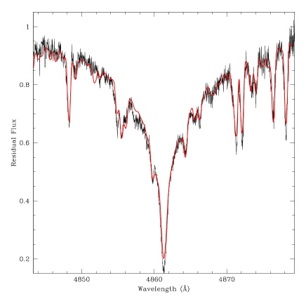
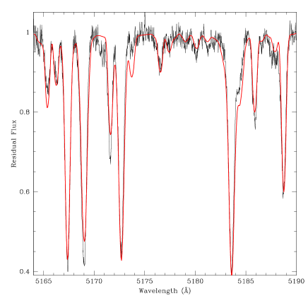
Figure 2: Two portions of observed spectrum matched to a model with $T_{\rm eff}$ = 6700, $\log g$ = 3.7 (red line). In the left panel we show the region around H$\beta$ that is sensitive to temperature, and in the right panel the region around Mgi triplet sensitive to gravity.

Statistical analyses of several $\delta$ Sct stars observed from the ground have already shown that the photometrically observed frequencies are not distributed at random, but that the excited nonradial modes cluster around the frequencies of the radial modes over many radial orders. The observed regularities can be partly explained by modes trapped in the stellar envelope (Breger, Lenz & Pamyatnykh, 2009). This leads to regularities in the observed frequency spectra, but not to exact equidistance.

In examining the Kepler data for $\delta$ Sct stars we noticed several stars in which many exactly equally-spaced frequency components are present. There are natural explanations for nearly equally spaced frequency multiplets such as harmonics and non-linear combination frequencies. In some of these stars, however, these mechanisms do not explain the spacings. In these stars there is often more than one exact frequency spacing and these are interleaved in a way which so far defies any explanation.

Some examples of equally-spaced frequency components which remain unexplained are known from ground-based observations. The $\delta$ Sct star 1 Mon has a frequency triplet where the departure from equidistance is extremely small: only $0.000079\pm 0.000001$ d^-1 (or $0.91\pm 0.01$ nHz), yet the frequency splitting cannot be due to rotation because $\ell=0$ for the central component and $\ell=1$ for the other two modes (Breger & Kolenberg, 2006; Balona et al., 2001). In the $\beta$ Cep star 12 Lac, there is a triplet with side peaks spaced by 0.1558 and 0.1553 d^-1. The probability that this is a chance occurrence is very small, yet photometric mode identification shows that two of these modes are $\ell=2$ and the third is $\ell=1$. This is therefore not a rotationally split triplet either (Handler et al., 2006).

One solution to these puzzling equally-spaced frequencies could be non-linear mode interaction through frequency locking. Buchler, Goupil & Hansen (1997) show that frequency locking within a rotationally split multiplet of a rapidly rotating star (150 to 200 km s^-1) could yield equally-spaced frequency splitting, which is to be contrasted to the prediction of linear theory where strong departures from equal splitting are expected.

In this paper we present a study of the $\delta$ Sct star KIC 9700322 (RA = 19:07:51, Dec = 46:29:12 J2000, Kp = 12.685). There are two modes with amplitudes exceeding 20000 ppm and several more larger than 1000 ppm. The equal frequency spacing is already evident in these large amplitude modes. This star does not fall in the unexplained category discussed above. It is, however, a remarkable example of a star in which combination frequencies are dominant.

The star has a large pulsational amplitude which can easily be observed from the ground. It was found to be variable in the ”All Sky Automated Survey” (Pigulski et al., 2008), where it is given the designation ASAS 190751+4629.2. It is classified as a periodic variable (PER) with a frequency of 7.79 d^-1. This is the 2 d^-1 alias of the main frequency (9.79 d^-1), which is determined below from the Kepler data. The Kepler data is, of course, not affected by daily aliasing. It was also examined during the ”Northern Sky Variability Survey” (Woźniak et al., 2004) with up to two measurements per night. Due to the short periods of the star, the 109 points of NSVS 5575265 were not suitable for a comparison with our results.

2 New observations of KIC 9700322

This star was observed with the Kepler satellite for 30.3 d during quarter 3 (BJD $245\,5093.21-245\,5123.56$) with short cadence. An overview of the Kepler Science Processing Pipeline can be found in Jenkins et al. (2010). The field crowding factor given in the KAC is 0.016, which is about the average for the Kepler field. The data were filtered by us for obvious outliers. After prewhitening the dominant modes, a number of additional points were rejected with a four-sigma filter as determined from the final multifrequency solution. 42990 out of 43103 data points could be used. We emphasize that most rejected points are extreme outliers and that the present conclusions do not change if no editing is performed. As can be expected from near-continuous set of observations with one measurement per minute, the spectral window is very clean with the second highest peak at 0.046 d^-1 and a height of 22% relative to the main peak.

A small, typical sample of the Kepler measurements is shown in Fig. 1. Inspection of the whole light curve indicates that the pattern shown in Fig. 1 is repeated every 0.72 d. The repetition, however, is not perfect. This simple inspection already suggests, but does not prove, that most of the variability is caused by a few dominant modes and that additional, more complex effects are also present.

The (Woźniak et al., 2004) Input Catalogue also does not list any photometry for this star, but some information on the spectral energy distribution is available. The spectral energy distribution was constructed using literature photometry: 2MASS (Skrutskie et al., 2006), GSC2.3 $B$ and $R$ (Lasker et al., 2008), TASS $V$ and $I$ (Droege et al., 2006), and CMC14 $r^{\prime}$ (Evans, Irwin & Helmer, 2002) magnitudes. Interstellar Na D lines present in the spectrum have equivalent widths of 60 $\pm$ 15 mÅ and 115 $\pm$ 20 mÅ for the D₁ and D₂ lines, respectively. The calibration of Munari & Zwitter (1997) gives $E(B-V)$= 0.03 $\pm$ 0.01.

The dereddened spectral energy distribution was fitted using solar-composition (Kurucz, 1993a) model fluxes. The model fluxes were convolved with photometric filter response functions. A weighted Levenberg-Marquardt non-linear least-squares fitting procedure was used to find the solution that mimimized the difference between the observed and model fluxes. Since the surface gravity is poorly constrained by our spectral energy distribution, fits were performed for $\log g=4.5$ and $\log g=2$ to assess the uncertainty due to unconstrained $\log g$. A final value of $T_{\rm eff}=7140\pm 310$ K was found. The uncertainties in $T_{\rm eff}$ includes the formal least-squares error and that from the uncertainties in $E(B-V)$ and $\log g$. We note here that in the next section values with considerably smaller uncertainties are determined from high-dispersion spectroscopy.

3 Characterization of the stellar atmosphere

In order to classify the star with higher precision and to test the very low rotational velocity predicted by our interpretation of the pulsation spectrum in later sections, a high-dispersion spectrum is needed. KIC 9700322 was observed on 2010 August 12 with the High Resolution Spectrograph (Tull, 1998) on the Hobby-Eberly Telescope at McDonald Observatory. The spectrum was taken at $R\sim 30\,000$ using the 316g cross-disperser setting, spanning a wavelength region from $4120-7850$Å. The exposure time was 1800 secs. A signal/noise ratio of 194 was found at 593.6 nm. We reduced the data using standard techniques with IRAF routines in the echelle package. These included overscan removal, bias subtraction, flat-fielding, order extraction, and wavelength calibration. The cosmic ray effects were removed with the L.A. Cosmic package (van Dokkum, 2001).

The effective temperature, $T_{\rm eff}$, and surface gravity, $\log g$, can be obtained by minimizing the difference between the observed and synthetic spectra. We used a fit to the H$\beta$ line to obtain an estimate of the effective temperature. For stars with $T_{\rm eff}<7000$ K the Balmer lines are no longer sensitive to gravity, so we used the Mgi triplet at 5167.321, 5172.684, and 5183.604 Å for this purpose. The goodness-of-fit parameter, $\chi^{2}$, is defined as

$\displaystyle\chi^{2}=\frac{1}{N}\sum\bigg{(}\frac{I_{\rm obs}-I_{\rm th}}{\delta I_{\rm obs}}\bigg{)}^{2}$,

where $N$ is the total number of points and $I_{\rm obs}$ and $I_{\rm th}$ are the intensities of the observed and computed profiles, respectively. $\delta I_{\rm obs}$ is the photon noise. The error in a parameter was estimated by the variation required to change $\chi^{2}$ by unity. The projected rotational velocity and the microturbulence were determined by matching the metal lines in the range 5160 – 5200 Å.

From this procedure we obtained T_eff = 6700 $\pm$ 100 K, $\log g$ = 3.7 $\pm$ 0.1, $v\sin i$ = 19 $\pm$ 1 km s^-1, $\xi$ = 2.0 $\pm$ 0.5 km s^-1. In Fig. 2, we show the match to observed spectrum. The theoretical profiles were computed with SYNTHE (Kurucz & Avrett, 1981) using ATLAS9 atmospheric models (Kurucz, 1993b). The solar opacity distribution function was used in these calculations. The effective temperature calculated from the spectrum is somewhat lower than that obtained by matching the spectral energy distribution discussed in the previous section. The difference is within the statistical uncertainties. We note that the spectrum showed no evidence for the presence of a companion.

Because of problems of line blending, we decided to use direct matching of rotationally-broadened synthetic spectra to the observations in order to determine the projected rotational velocity. For this purpose, we divided the spectrum into several 100 Å segments. We derived the abundances in each segment using $\chi^{2}$ minimization. We used the line lists and atomic parameters in Kurucz & Bell (1995) as updated by Castelli & Hubrig (2004).

Table 1 shows the abundances expressed in the usual logarithmic form relative to the total number of atoms $N_{\rm tot}$. To more easily compare the chemical abundance pattern in KIC 9700322, Fig. 3 shows the stellar abundances relative to the solar values (Grevesse et al., 2010) as a function of atomic number. The error in abundance for a particular element which is shown in Table 1 is the standard error of the mean abundance computed from all the wavelength segments. This analysis shows that the chemical abundance in KIC 9700322 is the normal solar abundance.

The effective temperature determined for KIC 9700322 makes the star one of the cooler $\delta$ Sct stars. Other pulsators with similar temperatures are known, e.g., 6700 K for $\rho$ Pup (Netopil et al., 2008) and 6900 K for 44 Tau (Lenz et al., 2010).

Figure 3: Abundance pattern derived for KIC 9700322.

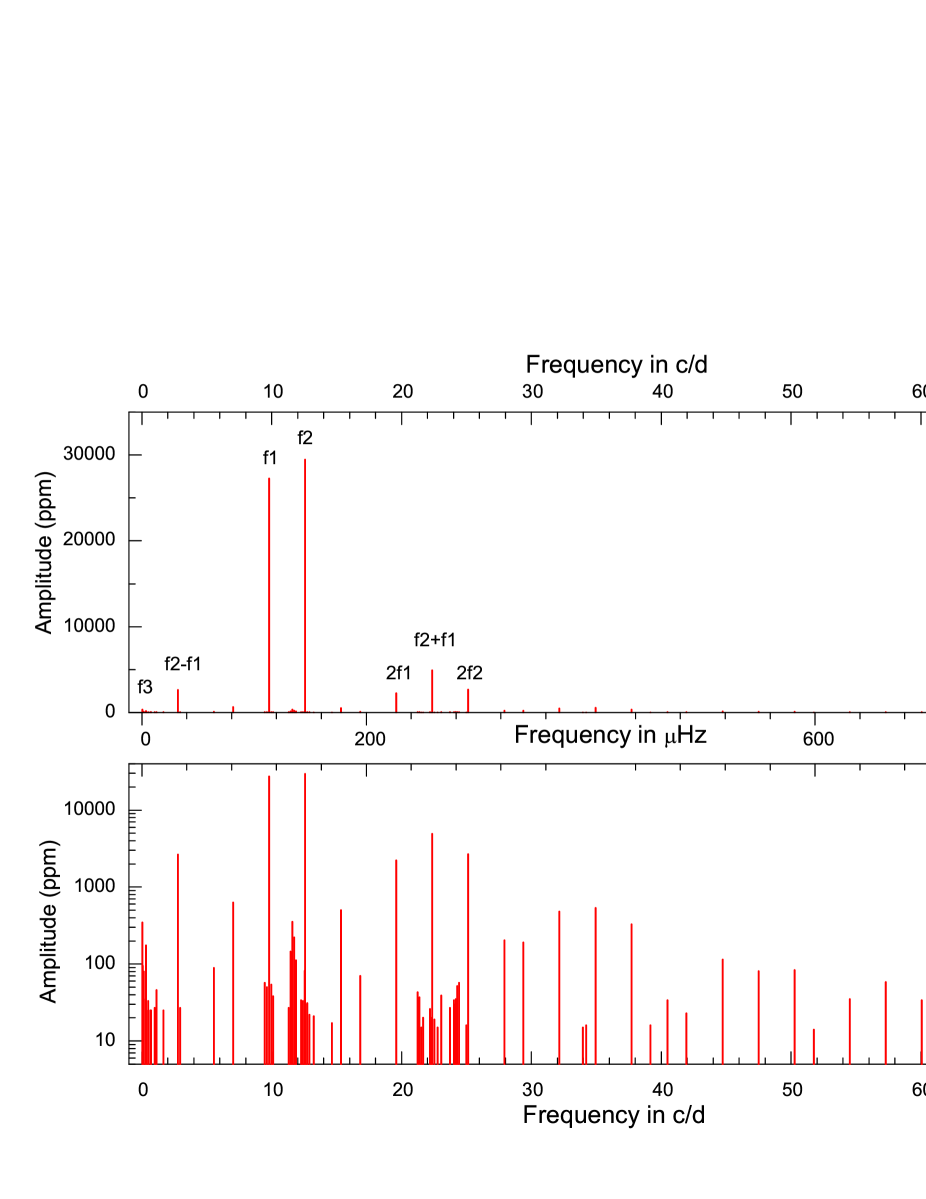
Figure 4: Amplitude spectra of KIC 9700322. The amplitudes (Table 2) are shown both linearly and logarithmically. The top panel illustrates the dominance of the two excited frequencies and that standard ground-based photometry would only detect these and a few combinations.

Table 1: Abundances derived for KIC 9700322 expressed in term of $\log N(el)/N_{\rm tot}$

C	$-$3.6 $\pm$ 0.3	Sc	$-$9.0 $\pm$ 0.3	Co	$-$6.8 $\pm$ 0.2
O	$-$3.1 $\pm$ 0.2	Ti	$-$7.2 $\pm$ 0.3	Ni	$-$5.8 $\pm$ 0.3
Na	$-$5.8 $\pm$ 0.3	V	$-$7.7 $\pm$ 0.3	Sr	$-$8.6 $\pm$ 0.1
Mg	$-$4.4 $\pm$ 0.4	Cr	$-$6.5 $\pm$ 0.2	Y	$-$9.4 $\pm$ 0.2
Si	$-$4.6 $\pm$ 0.1	Mn	$-$6.8 $\pm$ 0.2	Ba	$-$9.2 $\pm$ 0.4
Ca	$-$5.8 $\pm$ 0.4	Fe	$-$4.6 $\pm$ 0.2

4 Frequency analysis

The Kepler data of KIC 9700322 were analyzed with the statistical package PERIOD04 (Lenz & Breger, 2005). This package carries out multifrequency analyses with Fourier as well as least-squares algorithms and does not rely on the assumption of white noise. Previous comparisons of multifrequency analyses of satellite data with other techniques such as SIGSPEC (Reegen, 2007) have shown that PERIOD04 is more conservative in assigning statistical significances, leads to fewer (Poretti et al., 2009), and hopefully also fewer erroneous, pulsation frequencies, but may consequently also miss some valid frequencies.

We did not concern ourselves with small instrumental zero-point changes in the data since we have no method to separate these from intrinsic pulsation. Consequently, our solution contains several low frequencies in the region below 1 d^-1 which may only be mathematical artefacts of instrumental effects. The suspicion concerning the unreliable low frequencies is confirmed when comparing the present PERIOD04 results with those from other period search programs and different data editing.

Following the standard procedures for examining the peaks with PERIOD04, we have determined the amplitude signal/noise values for every promising peak in the amplitude spectrum and adopted a limit of S/N of 3.5. The value of 3.5 (rather than 4) could be adopted because most low peaks do not have random frequency values due to their origin as combinations. This standard technique is modified for all our analyses of accurate satellite photometry: the noise is calculated from prewhitened data because of the huge range in amplitudes of three orders of magnitudes.

After prewhitening 76 frequencies, the average residual per point was 430 ppm. The large number of measurements (42990) lead to very low noise levels in the Fourier diagrams as computed by PERIOD04: 7 ppm ($0-10$ d^-1), 4.7 ppm ($10-20$ d^-1), 3.9 ppm ($20-40$ d^-1), and 3.6 ppm ($40-200$ d^-1). At low frequencies the assumption of white noise is not realistic.

Table 2: Multifrequency solution of KIC 9700322 and identifications. Frequencies are given in cycles d^-1 and also in $\mu$Hz. Amplitudes are in parts per million (ppm).

Frequency		Amplitude	Identification	Comment	Frequency		Amplitude	Identification
d-1	$\mu$Hz	ppm			d-1	$\mu$Hz	ppm
$\pm$ 0.00021	$\pm$ 0.0021	$\pm$ 32
Main frequencies
9.7925	113.339	27266	$f_{1}$	Dominant mode
12.5688	145.472	29463	$f_{2}$	Dominant mode
0.1597	1.848	80	$f_{3}$	Rotation, causes combinations
11.3163	130.975	27	$f_{4}$	Quintuplet
11.4561	132.593	145	$f_{5}$	Quintuplet
11.5940	134.190	354	$f_{6}$	Quintuplet
11.7200	135.648	221	$f_{7}$	Quintuplet
11.8593	137.261	112	$f_{8}$	Quintuplet
Combination frequencies
0.3194	3.697	174	$2f_{3}$		22.7723	263.588	15	$f_{4}+f_{5}$
0.4791	5.545	33	$3f_{3}$		23.0501	266.719	39	$f_{5}+f_{6}$
0.6388	7.394	25	$4f_{3}$		23.7187	274.522	27	$2f_{8}$
0.7095	8.211	25	$f_{2}-f_{8}$		24.0249	278.066	34	$f_{5}+f_{2}$
0.9748	11.282	27	$f_{2}-f_{6}$		24.1628	279.662	35	$f_{6}+f_{2}$
1.1127	12.879	46	$f_{2}-f_{5}$		24.2888	281.120	52	$f_{7}+f_{2}$
1.6636	19.254	25	$f_{5}-f_{1}$		24.4282	282.733	57	$f_{8}+f_{2}$
2.7763	32.133	2633	$f_{2}-f_{1}$		24.9779	289.096	16	$2f_{2}-f_{3}$
2.9360	33.981	27	$f_{2}-f_{1}+f_{3}$		25.1376	290.945	2663	$2f_{2}$
5.5526	64.266	89	$2f_{2}-2f_{1}$		27.9139	323.078	203	$3f_{2}-f_{1}$
7.0162	81.206	632	$2f_{1}-f_{2}$		29.3776	340.018	191	$3f_{1}$
9.4731	109.643	57	$f_{1}-2f_{3}$		32.1538	372.151	479	$2f_{1}+f_{2}$
9.6328	111.491	50	$f_{1}-f_{3}$		33.9554	393.002	15	$f_{6}+f_{1}+f_{2}$
9.9522	115.188	54	$f_{1}+f_{3}$		34.2207	396.073	16	$f_{8}+f_{1}+f_{2}$
10.1119	117.036	38	$f_{1}+2f_{3}$		34.9301	404.284	536	$f_{1}+2f_{2}$
12.2494	141.775	34	$f_{2}-2f_{3}$		37.7064	436.417	329	$3f_{2}$
12.4091	143.624	33	$f_{2}-f_{3}$		39.1701	453.357	16	$4f_{1}$
12.7285	147.321	31	$f_{2}+f_{3}$		40.4827	468.550	34	$4f_{2}-f_{1}$
12.8882	149.169	22	$f_{2}+2f_{3}$		41.9464	485.490	23	$3f_{1}+f_{2}$
15.3451	177.605	502	$2f_{2}-f_{1}$		44.7227	517.623	114	$2f_{1}+2f_{2}$
16.8088	194.546	70	$3f_{1}-f_{2}$		47.4989	549.756	81	$f_{1}+3f_{2}$
19.5850	226.679	2225	$2f_{1}$		50.2752	581.889	83	$4f_{2}$
21.2486	245.933	43	$f_{5}+f_{1}$		54.5152	630.963	35	$3f_{1}+2f_{2}$
21.3865	247.529	37	$f_{6}+f_{1}$		57.2915	663.096	58	$2f_{1}+3f_{2}$
21.5125	248.987	15	$f_{7}+f_{1}$		60.0678	695.229	34	$f_{1}+4f_{2}$
21.6519	250.600	20	$f_{8}+f_{1}$		62.8440	727.362	15	$5f_{2}$
22.2016	256.963	26	$f_{1}+f_{2}-f_{3}$		67.0840	776.435	19	$3f_{1}+3f_{2}$
22.3613	258.812	4902	$f_{1}+f_{2}$		69.8603	808.568	21	$2f_{1}+4f_{2}$
22.5210	260.660	19	$f_{1}+f_{2}+f_{3}$
Other peaks in the amplitude spectrum
0.0221	0.256	347	$f_{66}$		13.2417	153.260	21	$f_{72}$
0.0555	0.642	95	$f_{67}$		14.6254	169.275	17	$f_{73}$
0.1346	1.558	35	$f_{68}$	$f_{4}$-$f_{5}$ and $f_{5}$-$f_{6}$?	22.3250	258.391	20	$f_{74}$
0.3542	4.100	25	$f_{69}$		24.1464	279.473	30	$f_{75}$
12.5347	145.077	82	$f_{70}$		51.7521	598.982	14	$f_{76}$
12.5837	145.645	30	$f_{71}$

¹ Accuracy of frequencies determined experimentally (see Section 4.1), independent of amplitude. The numbers apply only to unblended frequency peaks. Because of the high quality of the $Kepler$ data, the frequency accuracy is much better than the resolution calculated from the length of a 30.3 d run.

² Determined by a multiple-frequency least-squares solution.

Our analysis was performed using intensity units (ppm). The analysis was repeated with the logarithmic units of magnitudes, which are commonly used in astronomy. The differences in the results were, as expected, minor and have no astrophysical implications. The only small difference beyond the scaling factor of 1.0857 involved neighboring peaks with large intensity differences, in which the weaker peak was in an extended ’wing’ of the dominant peak: the effects are numerical from the multiple-least-squares solutions.

KIC 9700322 shows only six frequencies with amplitudes larger than 1000 ppm, of which only the two main frequencies are independent. Although a few ground-based campaigns lasting several years have succeeded in detecting statistically significant modes with smaller amplitudes, 1000 ppm can be regarded as a good general limit. Observed with standard ground-based techniques, the star would show few frequencies. In all, we find 76 statistically significant frequencies.

Figure 5: Echelle diagram of the detected frequencies using 2.7763 d^-1, which is the difference between the two dominant pulsation modes. All patterns can be easily explained through combination modes, rotational splitting and modulation (see text).

4.1 The observed frequency combinations

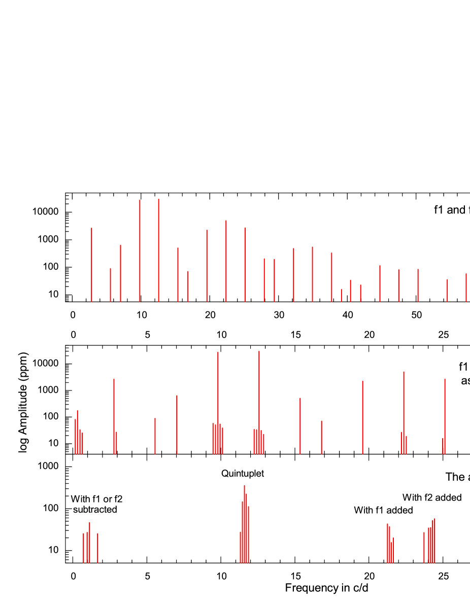
Figure 7: Top panel: Amplitude spectrum of those frequencies which are numerical combinations of the two dominant modes only. This demonstrates the richness of the combinations. Notice that the patterns are more complex than a simple Fourier sum. The middle panel demonstrates that some of those combination frequencies show further splittings with $f_{3}$ (rotation). The bottom panel shows an additional set of five frequencies together with the combinations of the set with $f_{1}$ and $f_{2}$.

Most of the detected frequencies can be identified as parts of regular patterns (see Fig. 7). Visual inspection shows that the most obvious pattern is the exact spacing of $\delta f=2.7763$ d^-1. This is confirmed by statistical analyses of all possible frequency differences present in the data. However, this pattern is not continued over the whole spectrum, but is present as different patterns, repeated and interleaved several times. Consequently, a simple explanation in terms of a Fourier series (e.g., of a nonsinusoidal light curve) is not applicable.

Fig. 5 shows the Echelle diagram using 2.7763 d^-1, which demonstrates the presence of remarkable patterns. Investigation of these patterns reveals that they originate in very simple frequency combinations and that the 2.7763 d^-1 is only a marker of the true explanation: combinations of the two dominant modes $f_{1}$ and $f_{2}$, as shown in Table 2. In fact, 2.7763 d^-1 = ($f_{2}-f_{1})$.

The frequencies shown in the top panel of Fig. 7 can be expressed in as very simple way through the equation $f=mf_{1}\pm nf_{2}$, where $m$ and $n$ are small integers. The fact that $f_{1}$ and $f_{2}$ are the two modes with the highest amplitudes makes this approach also physically reasonable (see below).

We also detect a frequency at 0.1597 d^-1 (called $f_{3}$). This frequency is important, since additional patterns are also seen: a number of peaks are separated by exactly the value of $f_{3}$ (see middle panel of Fig. 7).

Altogether, 57 frequencies can be identified as numerical combinations and multiples involving $f_{1}$, $f_{2}$ and $f_{3}$ by comparing the observed to the predicted frequencies. We can essentially rule out accidental agreements. Let us consider the combination frequencies at frequencies larger than 3 d^-1, where the noise figures in the amplitude spectrum are reliable. For our identifications the average deviation between the observed and predicted frequency value is only 0.00021 d^-1. Such agreement is remarkable if one considers that the Kepler measurements used a time base of only 30 d and that $1/T=0.03$ d^-1 where $T$ is the time span between the last and first observation. The present result is typical for Kepler satellite data.

If we use the least-squares frequency uncertainties calculated by PERIOD04, on average the observed agreement is 44$\%$ better than predicted. However, such calculations assume white noise, which is not warranted. We can adopt the formulae given in Kallinger, Reegen & Weiss (2008) for the upper limit of the frequency uncertainty to include frequency-dependent noise. We calculated signal/noise ratios in 5 d^-1 bins centred on each frequency with PERIOD04 using the prewhitened spectrum. With this more realistic approach, the observed deviation of 0.00021 d^-1 is exactly a factor of two lower than the statistical upper limit. This supports our identifications.

4.2 The quintuplet

Five almost equidistant frequencies in the $11-12$ d^-1 range are also present together with various combinations of these frequencies with $f_{1}$ and $f_{2}$. This is shown in the bottom panel of Fig. 7.

4.3 Explanation of the Echelle diagram

We can now explain the patterns seen in the Echelle diagram (Fig. 5) in a simple manner. The vertical structures are the combination frequencies involving $f_{1}$ and/or $f_{2}$. They are displaced from each other because different low integers of $m$ and $n$ (in the equation $f=mf_{1}\pm nf_{2}$) are involved. The horizontal structures with a slight incline correspond to the frequencies separated by $\sim$0.13 and 0.16 d^-1, which are connected with the rotational frequency of 0.1597 d^-1 through rotational splitting and modulation. The incline occurs because the small frequency differences between adjacent frequency values must show up in both the $x$ and $y$ directions of the diagram. Details on the values and identifications of the individual frequencies are listed in Table 2.

4.4 Additional frequencies

A few additional peaks have been identified, which are not related to $f_{1}-f_{8}$ in an obvious or unique manner. The lowest frequencies were already discussed earlier as probable zero-point drift and their values were dependent on how the data were reduced. The non-combination frequency at 51.75 d^-1 has an amplitude of only 14 ppm. Calculation of the noise around the frequency gives a signal/noise ratio of 3.6, which makes it a very marginal detection.

Fig. 6 shows the amplitude spectrum of the residuals after prewhitening of the 76 frequencies. No peak is statistically significant and the overall distribution of amplitudes is typical of noise. Nevertheless, we have examined the highest (not significant) peaks, since a few of these may be real. Three peaks can be identified with expected values of additional combination frequencies, e.g., a peak at 8.129 d^-1 can be fit by 2$f_{1}$-$f_{5}$ at an amplitude signal/noise ratio of 3.0.

Figure 6: Amplitude spectrum of KIC 9700322 after prewhitening 76 frequencies. Note the low amplitudes of any additional pulsation modes present in the star.

Table 3: The additional $l$=2 quintuplet: Observed separations

Frequency	Separation from central frequency
d-1	d-1
$\pm$ 0.0002	$\pm$ 0.0003
11.3163	-0.2777
11.4561	-0.1379
11.5940	0
11.7200	0.1260
11.8593	0.2653

5 Discussion

Although this star was selected because of its very clear exactly equal frequency spacing, it turns out that the frequency spacing is explained as simple combination frequencies arising from non-linearities of the oscillation. This is different from another class of $\delta$ Sct stars in the Kepler database which also show exact frequency spacings, but in a manner which is not at present understood. Examples of this strange class will be presented in a separate paper.

What makes KIC 9700322 interesting is the remarkable way in which the large number of frequencies are related to the two main frequencies, $f_{1}$ and $f_{2}$. This behaviour is very similar to the high amplitude $\delta$ Sct star KIC 9408694, also discovered in the Kepler database. The frequency patterns together with their amplitudes permit us to identify the different frequencies and to provide physical interpretations.

5.1 The dominant radial modes

The period ratio of $f_{1}$ and $f_{2}$ is 0.779. This is close to the expected period ratio for fundamental and first overtone radial pulsation. The pulsation amplitudes of $\delta$ Sct stars increase with decreasing rotation, e.g., see Fig. 5 of Breger (2000). Furthermore, high amplitudes occur mainly in slowly rotating, radial pulsators: in fact, the high-amplitude $\delta$ Sct (HADS) subgroup is defined on the basis of peak-to-peak amplitudes in excess of 0.3 mag. Nevertheless, a rigid separation between radial HADS and lower-amplitude nonradial $\delta$ Sct stars does not exist. Dominant radial modes with amplitudes smaller than 0.3 mag have previously been found. Examples of EE Cam (Breger, Rucinski & Reegen, 2007) and 44 Tau (Lenz et al., 2010). The situation might be summarized as follows: Dominant radial modes occur only in slowly rotating stars.

Since KIC 9700322 is sharp-lined ($v\sin i=19$ km s^-1) and presumably also a slow rotator, it follows this relationship. The presence of two dominant radial modes with amplitudes less than the HADS limits of peak-to-peak amplitudes of 0.3 mag is not unusual.

The measured $v\sin i$ value supports the interpretation of the observed 0.1597 d^-1 peak as the rotational frequency. In fact, both dominant modes have very weak side lobes with spacings of exactly the rotational frequency. The side lobes are very weak: for $f_{1}$ and $f_{2}$ the amplitudes are only 0.0018 and 0.0011 of the central peak amplitudes. We interpret this as a very small modulation of the amplitudes with rotation. An alternate explanation in terms of rotational splitting of nonradial modes is improbable because rotational splitting does not lead to exact frequency separation unless there is frequency locking due to resonance. Also, the extreme amplitude ratios tend to favour the interpretation in terms of amplitude modulation.

Based on this mode identification assumption we investigated representative asteroseismic models of the star. We have used two independent numerical packages: the first package consisted of the current versions of the Warsaw-New Jersey stellar evolution code and the Dziembowski pulsation code (Dziembowski, 1977; Dziembowski & Goode, 1992). The second package is composed by the evolutionary code cesam (Morel, 1997), and the oscillation code filou (Suárez, 2002; Suárez, Goupil & Morel, 2006). Both pulsation codes consider second-order effects of rotation including near degeneracy effects.

The period ratio between the first radial overtone and fundamental mode mainly depends on metallicity, rotation and stellar mass. Moreover, the radial period ratio also allows for inferences on Rosseland mean opacities as shown in Lenz et al. (2010).

Indeed, an attempt to reproduce the radial fundamental and first overtone mode at the observed frequencies with the first modelling package revealed a strong dependence on the choice of the chemical composition and the OPAL vs. OP opacity data (Iglesias & Rogers, 1996; Seaton, 2005). The best model found in this investigation was obtained with OP opacities and increased helium and metal abundances. Unfortunately, this model ($T_{\rm eff}=7400$ K, $\log L/{\rm L}_{\odot}=1.27$, $\log g=3.87$, 2M_⊙) is much hotter than observations indicate. The disagreement in effective temperature indicates that this model is not correct despite the good fit of the radial modes.

As an additional test, by adopting the radial linear nonadiabatic models developed by Marconi & Palla (1998) and Marconi et al. (2004), we are able to reproduce the values of the two dominant frequencies with pulsation in the fundamental and first overtone modes, but with a lower period ratio (0.770) than observed. The best fit solution obtained with these models, for an effective temperature consistent with the spectroscopic determination and assuming solar chemical composition, corresponds to: $M=1.65M_{\odot}$, $\log L/{\rm L}_{\odot}=1.1$, $T_{\rm eff}=6700$ K, $\log g=3.83$. We notice that for this combination of stellar parameters, both the fundamental and the first overtone mode are unstable in these models. Moreover, looking at the Main Sequence and post-Main Sequence evolutionary tracks in the gravity versus effective temperature plane, as reported in Fig. 4 of Catanzaro et al. (2010), the solution $T_{\rm eff}$ = 6700 K, $\log g=3.83$ is consistent with a $1.65M_{\odot}$ stellar mass.

However, as already noted, the period ratio in our models is lower than the observed value. To resolve this discrepancy, the possibility of low metallicity and rotation effects was examined in more detail with the second modeling package. Models between $T_{\rm eff}=6200$ K and $8600\,$K with masses between 1.2 and 1.76${\rm M}_{\odot}$, were found to represent a good fit of $f_{1}$ and $f_{2}$ as radial fundamental and first overtone, respectively. The best fit with the observations was found for $M=1.2\,{\rm M}_{\odot}$ models computed with $\alpha_{\rm MLT}=0.5$, ${\rm d}_{ov}=0.1$, and a metallicity of [Fe/H] = -0.5 dex. Such a low value for the convection efficiency is in good agreement with the predictions by Casas et al. (2006) for $\delta$ Sct stars, based on their non-adiabatic asteroseismic analysis. All these parameters roughly match the general characteristics of the $\delta$ Sct stars with dominant radial modes and large amplitudes, despite being in the limit in metallicity.

The $P_{1}/P_{0}$ period ratios predicted by these models (which simultaneously fit $P_{0}$) are near 0.775, which is lower than the observed ratio, 0.779. A period ratio of 0.775 is also obtained by adopting the radial linear nonadiabatic models by Marconi et al. (2004) at $Z=0.006$, according to which the best fit solution with effective temperature consistent with the spectroscopic determination, corresponds to $Z=0.006$, $Y=0.25$, $M=1.5$, $\log L/L_{\odot}=1.04$, $T_{e}=6700$ K, $\log g=3.83$. Again the fundamental and first overtone modes are predicted to be simultaneoulsy unstable for this parameter combination. We explored the possibility that such a discrepancy might be due to rotation effects, particularly second-order distortion effects, as discussed by Suárez, Garrido & Goupil (2006) and Suárez, Garrido & Moya (2007). These investigations analyze theoretical Petersen Diagrams including rotation effects (Rotational Petersen Diagrams, hereafter RPDs), and show that $P_{1}/P_{0}$ ratios increase as stellar surface rotation increases. The rotation rate derived from observations is slightly below 25 km s^-1 (see section 5.3). At such rotation rates near degeneracy effects on the period ratio are small (less than 0.001 in $P_{1}/P_{0}$). However, when non-spherically symmetric components of the centrifugal force are considered, near-degeneracy effects may be larger, around 0.0025, causing the presence of wriggles in the RPDs (see Fig. 5 in Suárez, Garrido & Moya (2007) and Fig. 6 in Pamyatnykh (2003)). Such effects are even more significant for rotational velocities higher than 40 - 50 km s^-1. Consequently, near-degeneracy effects may help to decrease the discrepancy between the observed period ratio and the slightly lower values predicted by the models.

If the star had a low metal abundance (close to Pop. II), a detailed analysis of RPDs might have provided an independent estimate of the true rotational velocity (and thereby of the angle of inclination). However, the spectroscopic analysis indicates that the star has a solar abundance. KIC 9700322 therefore represents a challenge to asteroseismic modeling, since it appears impossible to reproduce all observables simultaneously with standard models.

5.2 The combination frequencies

We have already shown that the 50+ detected frequency peaks can be explained by simple combinations of the two dominant modes and the rotational frequency. Several different nonlinear mechanisms may be responsible for generating combination frequencies between two independent frequencies, $\nu_{1}$ and $\nu_{2}$. For example, any non-linear transformation, such as the dependence of emergent flux variation on the temperature variation ($L=\sigma T^{4}$) will lead to cross terms involving frequencies $\nu_{1}+\nu_{2}$ and $\nu_{1}-\nu_{2}$ and other combinations. The inability of the stellar medium to respond linearly to the pulsational wave is another example of this effect. Combination frequencies may also arise through resonant mode coupling when $\nu_{1}$ and $\nu_{2}$ are related in a simple numerical way such as $2\nu_{1}\approx 3\nu_{2}$.

The interest in the combination frequencies derives from the fact that their amplitudes and phases may allow indirect mode identification. For nonradial modes, some combination frequencies are not allowed depending on the parity of the modes (Buchler, Goupil & Hansen, 1997) which could lead to useful constraints on mode identification. Since $f_{1}$ and $f_{2}$ in KIC 9700322 are both presumably radial, there are no such constraints.

The identification of $f_{1}$ and $f_{2}$ with radial modes allows us to investigate the properties of the Fourier parameters of the combination modes with the aim to disentangle less obvious cases and/or solutions with a smaller number of combination terms. Buchler, Goupil & Hansen (1997) show that a resonance of the type $f_{c}=n_{1}f_{1}+n_{2}f_{2}$ leads to a phase $\phi_{r}=\phi_{c}-(n_{1}\phi_{1}+n_{2}\phi_{2})$. In the same way we may define the amplitude ratios $A_{r}=A_{c}/(A_{1}A_{2})$. To investigate how $\phi_{r}$ and $A_{r}$ behave with frequency, we first need the best estimate of the parent frequencies. We obtained these by non-linear minimization of a truncated Fourier fit involving $f_{1},f_{2}$ and all combination frequencies up to the 4^th order. The best values are $f_{1}=9.792514$ and $f_{2}=12.568811$ d^-1. The resulting amplitude and phases are shown in Table 4 together with the values of $\phi_{r}$ and $A_{r}$. The phases were calculated relative to BJD 245 5108.3849 which corresponds to the midpoint of the observations.

Table 4: Best fitting amplitudes, $A_{c}$ (ppm), and phases $\phi_{c}$ (radians), for the parent frequencies and their combination frequencies up to fourth order. Relative phases, $\phi_{r}$ and amplitudes, $A_{r}$ are also shown.

$(n_{1},n_{2})$	$f_{c}$	$A_{c}$	$\phi_{c}$	$\phi_{r}$	$A_{r}$
( 1, 0)	9.792514	27271	2.710
( 0, 1)	12.568811	29443	-1.313
( 2, 0)	19.585028	2225	-0.110	0.751	0.002553
( 1, 1)	22.361325	4898	1.954	0.557	0.005619
( -1, 1)	2.776297	2636	0.826	-1.431	0.003024
( 0, 2)	25.137622	2663	-2.317	0.310	0.003055
( 3, 0)	29.377542	192	-2.749	1.684	0.000222
( 2, 1)	32.153839	476	-0.835	1.339	0.000547
( 2, -1)	7.016217	633	0.127	-0.324	0.000726
( 1, 2)	34.930136	536	0.202	0.119	0.000615
( -1, 2)	15.345108	502	0.525	-0.418	0.000577
( 0, 3)	37.706433	329	-0.658	-3.000	0.000377
( 4, 0)	39.170056	12	0.844	2.567	0.000014
( 3, 1)	41.946353	22	-2.748	2.999	0.000026
( 3, -1)	16.808731	69	-2.521	0.598	0.000080
( 2, 2)	44.722650	114	0.869	-1.924	0.000132
( -2, 2)	5.552594	87	-2.717	-0.951	0.000101
( 1, 3)	47.498947	84	-1.941	-0.710	0.000097
( -1, 3)	27.913919	205	0.199	0.568	0.000236
( 0, 4)	50.275244	84	-1.061	-2.088	0.000097

Figure 8: The relative amplitudes, $A_{r}$, and phases, $\phi_{r}$ (radians) as a function of frequency (d^-1). The dotted lines show the location of the parent frequencies.

Fig. 8 shows how $A_{r}$ and $\phi_{r}$ vary with frequency. From the figure we note that $A_{r}$ is largest for $f_{1}+f_{2}$, $2f_{1}$, $2f_{2}$ and $f_{2}-f_{1}$ and very small for the rest. It is also interesting that $\phi_{r}$ is a relatively smooth function of frequency, being practically zero in the vicinity of the parent frequencies, decreasing towards smaller frequencies and increasing towards higher frequencies. This result is almost independent of the choice of $f_{1}$ and $f_{2}$. The standard deviation of $f_{1}$ and $f_{2}$ is 0.0001 d^-1 using the Montgomery & O’Donoghue (1999) formula. One may arbitrarily adjust $f_{1}$ and $f_{2}$ in opposite directions by this value, and using the corresponding calculated values of the combination frequencies, fit the data to obtain new phases. The resulting $\phi_{r}$ versus frequency remains monotonic, but the slope does change. The smooth monotonic nature of the $\phi_{r}$ versus frequency diagram remains even for a change of ten times the standard deviation in opposite directions for $f_{1}$ and $f_{2}$ and for arbitrary changes in epoch of phase zero. The result is clearly robust to observational errors, but it is not clear what physical conclusions may be derived from this result. The behaviour is certainly not random and must have a physical basis. Note that for simple trigonometric products, $\phi_{r}$ will always be zero.

Finally, we note that the amplitudes of the combination modes relative to the amplitudes of their parents can be compared with values detected in the star 44 Tau (Breger & Lenz, 2008). They agree to a factor of two or better, suggesting that KIC 9700322 is not unusual in this regard, just more accurately studied because of the Kepler data.

5.3 The quintuplet

In addition to the quintuplet structure around the two dominant modes another quintuplet with different properties is present in KIC 9700322 (see the listing of $f_{4}$ to $f_{8}$ in Table 3). The average spacing between the frequencies in this quintuplet is slightly smaller than the rotational frequency (0.1338 d^-1 vs. 0.1597 d^-1). This makes this quintuplet different from the quintuplet structures found around the two dominant modes, which exhibit a spacing that corresponds exactly to the rotation frequency. Moreover, the distribution of amplitudes within the third quintuplet is fundamentally different to the patterns around $f_{1}$ and $f_{2}$. The given characteristics support an interpretation of the quintuplet as an $l$ = 2 mode.

The location of the quintuplet near the centre in between the radial fundamental and first overtone mode rules out pure acoustic character. Consequently, the observed quintuplet consists of mixed modes with considerable kinetic energy contribution from the gravity-mode cavity. For such modes theory predicts a smaller (and more symmetrical) rotational splittings compared to acoustic modes due to different values of the Ledoux constant $C_{nl}$. Using the framework of second order theory (Dziembowski & Goode, 1992) we determined the equatorial rotation rate which provides the best fit of the observed quintuplet with an $\ell=2$ multiplet. The best results were obtained for an equatorial rotation rate of 23 km s^-1. This is only slightly higher than the observed $v\sin i$ value of 19 km s^-1, and therefore indicates a near-equator-on-view. The Ledoux constant, $C_{nl}$, of the $\ell=2$ quintuplet is 0.164. For quadrupole modes $C_{nl}$ ranges between $\approx$0.2 for pure gravity modes to smaller values for acoustic modes. With (1 - $C_{nl}$) = 0.836 this leads to a rotational frequency, $\nu_{rot}=\frac{\Omega}{2\Pi}$, of around 0.16 d^-1. Consequently, this theoretical result confirms the interpretation of $f_{3}$ as a rotational feature and of the quintuplet as $l$ = 2 modes. Further support is provided by the fact that we see various combinations of the quintuplet with $f_{1}$ and $f_{2}$.

Moreover, the location of the quintuplet allows us to determine the extent of overshooting from the convective core. In the given model we obtained $\alpha_{ov}=0.13$ but the uncertainties elaborated in Section 5.1 currently prevent an accurate determination.

5.4 Further discussion

A remarkable aspect of the star is the fact that so few pulsation modes are excited with amplitudes of 10 ppm or larger.

In the interior of an evolved $\delta$ Sct star, even high-frequency $p$ modes behave like high-order $g$ modes. The large number of spatial oscillations of these modes in the deep interior leads to severe radiative damping. As a result, nonradial modes are increasingly damped for more massive $\delta$ Sct stars, which explains why high-amplitude$\delta$ Sct stars pulsate in mostly radial modes and why in even more massive classical Cepheids nonradial modes are no longer visible.

In general, we do not expect the frequencies in the $\delta$ Sct stars observed by Kepler to be regularly spaced because, unlike ground-based photometry, the observed pulsation modes are not limited to small spherical harmonic degree, $l$. For the very low amplitudes detected by Kepler we may expect to see a large number of small-amplitude modes with high $l$. The observed amplitudes decreases very slowly with $l$ and, all things being equal, a large number of modes with high $l$ might be expected to be seen in $\delta$ Sct and other stars (Balona & Dziembowski, 1999). The $\delta$ Sct stars HD 50844 (Poretti et al., 2009) and HD 174936 (García Hernández et al., 2009) observed by CoRoT show many hundreds of closely-spaced frequencies and may be examples of high-degree modes. The relatively small number of independent frequencies detected in KIC 9700322 stands in strong contrast to the two stars observed by CoRoT.

It should be noted that, unlike many $\delta$ Sct stars observed by Kepler, KIC 9700322 does not have any frequencies in the range normally seen in $\gamma$ Dor stars. The only strong frequencies in this range are a few combination frequencies. Although we have identified significant frequencies below 0.5 d^-1, it is not possible at this stage to verify whether these are due to the star or instrumental artefacts. At present, we do not understand why low frequencies are present in so many $\delta$ Sct stars.

Regularities in the frequency spacing due to combination modes have already been observed from the ground even in low amplitude $\delta$ Sct stars. An example is the star 44 Tau (Breger & Lenz, 2008). Fig. 2 of Breger, Lenz & Pamyatnykh (2009) demonstrates that all the observed regularities outside the $5-13$ d^-1 range are caused by combination modes. For combination modes the frequency spacing must be absolutely regular within the limits of measurability. This is found for KIC 9700322.

References

- Balona et al. (2001) Balona L. A. et al., 2001, MNRAS, 321, 239
- Balona & Dziembowski (1999) Balona L. A., Dziembowski W. A., 1999, MNRAS, 309, 221
- Breger (2000) Breger M., 2000, in Astronomical Society of the Pacific Conference Series, Vol. 210, Delta Scuti and Related Stars, M. Breger & M. Montgomery, ed., p. 3
- Breger & Kolenberg (2006) Breger M., Kolenberg K., 2006, A&A, 460, 167
- Breger & Lenz (2008) Breger M., Lenz P., 2008, A&A, 488, 643
- Breger, Lenz & Pamyatnykh (2009) Breger M., Lenz P., Pamyatnykh A. A., 2009, MNRAS, 396, 291
- Breger, Rucinski & Reegen (2007) Breger M., Rucinski S. M., Reegen P., 2007, AJ, 134, 1994
- Buchler, Goupil & Hansen (1997) Buchler J. R., Goupil M., Hansen C. J., 1997, A&A, 321, 159
- Casas et al. (2006) Casas R., Suárez J. C., Moya A., Garrido R., 2006, A&A, 455, 1019
- Castelli & Hubrig (2004) Castelli F., Hubrig S., 2004, A&A, 425, 263
- Catanzaro et al. (2010) Catanzaro G. et al., 2010, MNRAS, 1732
- Droege et al. (2006) Droege T. F., Richmond M. W., Sallman M. P., Creager R. P., 2006, PASP, 118, 1666
- Dupret et al. (2005) Dupret M., Grigahcène A., Garrido R., Gabriel M., Scuflaire R., 2005, A&A, 435, 927
- Dziembowski (1977) Dziembowski W., 1977, AcA, 27, 95
- Dziembowski & Goode (1992) Dziembowski W. A., Goode P. R., 1992, ApJ, 394, 670
- Evans, Irwin & Helmer (2002) Evans D. W., Irwin M. J., Helmer L., 2002, A&A, 395, 347
- García Hernández et al. (2009) García Hernández A. et al., 2009, A&A, 506, 79
- Gilliland et al. (2010) Gilliland R. L. et al., 2010, ApJ, 713, L160
- Grevesse et al. (2010) Grevesse N., Asplund M., Sauval A. J., Scott P., 2010, Ap&SS, 328, 179
- Grigahcène et al. (2010) Grigahcène A. et al., 2010, ApJ, 713, L192
- Handler et al. (2006) Handler G. et al., 2006, MNRAS, 365, 327
- Iglesias & Rogers (1996) Iglesias C. A., Rogers F. J., 1996, ApJ, 464, 943
- Jenkins et al. (2010) Jenkins J. M. et al., 2010, ApJ, 713, L87
- Kallinger, Reegen & Weiss (2008) Kallinger T., Reegen P., Weiss W. W., 2008, A&A, 481, 571
- Koch et al. (2010) Koch D. G. et al., 2010, ApJ, 713, L79
- Kurucz (1993a) Kurucz R., 1993a, ATLAS9 Stellar Atmosphere Programs and 2 km/s grid. Kurucz CD-ROM No. 13. Cambridge, Mass.: Smithsonian Astrophysical Observatory, 1993., 13
- Kurucz & Bell (1995) Kurucz R., Bell B., 1995, Atomic Line Data (R.L. Kurucz and B. Bell) Kurucz CD-ROM No. 23. Cambridge, Mass.: Smithsonian Astrophysical Observatory, 1995, 23
- Kurucz (1993b) Kurucz R. L., 1993b, in Astronomical Society of the Pacific Conference Series, Vol. 44, IAU Colloq. 138: Peculiar versus Normal Phenomena in A-type and Related Stars, M. M. Dworetsky, F. Castelli, & R. Faraggiana, ed., pp. 87–97
- Kurucz & Avrett (1981) Kurucz R. L., Avrett E. H., 1981, SAO Special Report, 391
- Lasker et al. (2008) Lasker B. M. et al., 2008, AJ, 136, 735
- Lenz & Breger (2005) Lenz P., Breger M., 2005, Communications in Asteroseismology, 146, 53
- Lenz et al. (2010) Lenz P., Pamyatnykh A. A., Zdravkov T., Breger M., 2010, A&A, 509, 90
- Marconi & Palla (1998) Marconi M., Palla F., 1998, ApJ, 507, L141
- Marconi et al. (2004) Marconi M., Ripepi V., Palla F., Ruoppo A., 2004, Communications in Asteroseismology, 145, 61
- Montgomery & O’Donoghue (1999) Montgomery M. H., O’Donoghue D., 1999, Delta Scuti Star Newsletter, 13, 28
- Morel (1997) Morel P., 1997, A&AS, 124, 597
- Munari & Zwitter (1997) Munari U., Zwitter T., 1997, A&A, 318, 269
- Netopil et al. (2008) Netopil M., Paunzen E., Maitzen H. M., North P., Hubrig S., 2008, A&A, 491, 545
- Pamyatnykh (2003) Pamyatnykh A. A., 2003, Ap&SS, 284, 97
- Pigulski et al. (2008) Pigulski A., Pojmanski G., Pilecki B., Szczygiel D., 2008, ArXiv e-prints
- Poretti et al. (2009) Poretti E. et al., 2009, A&A, 506, 85
- Reegen (2007) Reegen P., 2007, A&A, 467, 1353
- Seaton (2005) Seaton M. J., 2005, MNRAS, 362, L1
- Skrutskie et al. (2006) Skrutskie M. F. et al., 2006, AJ, 131, 1163
- Suárez (2002) Suárez J. C., 2002, Ph.D. Thesis, ISBN 84-689-3851-3, ID 02/PA07/7178
- Suárez, Garrido & Goupil (2006) Suárez J. C., Garrido R., Goupil M. J., 2006, A&A, 447, 649
- Suárez, Garrido & Moya (2007) Suárez J. C., Garrido R., Moya A., 2007, A&A, 474, 961
- Suárez, Goupil & Morel (2006) Suárez J. C., Goupil M. J., Morel P., 2006, A&A, 449, 673
- Tull (1998) Tull R. G., 1998, in Presented at the Society of Photo-Optical Instrumentation Engineers (SPIE) Conference, Vol. 3355, Society of Photo-Optical Instrumentation Engineers (SPIE) Conference Series, S. D’Odorico, ed., p. 387
- van Dokkum (2001) van Dokkum P. G., 2001, PASP, 113, 1420
- Woźniak et al. (2004) Woźniak P. R. et al., 2004, AJ, 127, 2436