PoS(Lattice 2010)122
DESY 10-222
Edinburgh 2010/30
Liverpool LTH 889

Flavour symmetry breaking and tuning the strange quark mass for 2+1 quark flavours

Abstract:

QCD lattice simulations with 2+1 flavours typically start at rather large up-down and strange quark masses and extrapolate first the strange quark mass to its physical value and then the up-down quark mass. An alternative method of tuning the quark masses is discussed here in which the singlet quark mass is kept fixed, which ensures that the kaon always has mass less than the physical kaon mass. Using group theory the possible quark mass polynomials for a Taylor expansion about the flavour symmetric line are found, which enables highly constrained fits to be used in the extrapolation of hadrons to the physical pion mass. Numerical results confirm the usefulness of this expansion and an extrapolation to the physical pion mass gives hadron mass values to within a few percent of their experimental values.

1 Introduction

The QCD interaction is flavour-blind. Neglecting electromagnetic and weak interactions, the only difference between quark flavours comes from the quark mass matrix. We investigate here how flavour-blindness constrains hadron masses after flavour $SU(3)$ is broken by the mass difference between the strange and light quarks, to help us extrapolate $2+1$ flavour lattice data to the physical point.

We have our best theoretical understanding when all $3$ quark flavours have the same masses (because we can use the full power of flavour $SU(3)$); nature presents us with just one instance of the theory, with $m_{s}^{\mbox{\tiny$R$}}/m_{l}^{\mbox{\tiny$R$}}\approx 25$. We are interested in interpolating between these two cases.

We consider possible behaviours near the symmetric point, and find that flavour blindness is particularly helpful if we approach the physical point, $(m_{l}^{\mbox{\tiny$R$}\,*},m_{s}^{\mbox{\tiny$R$}\,*})$, along a path in the $(m_{l}^{\mbox{\tiny$R$}},m_{s}^{\mbox{\tiny$R$}})$ plane starting at a point on the $SU(3)$ flavour symmetric line ($m_{l}^{\mbox{\tiny$R$}}=m_{s}^{\mbox{\tiny$R$}}$) and holding the sum of the quark masses $m_{u}^{\mbox{\tiny$R$}}+m_{d}^{\mbox{\tiny$R$}}+m_{s}^{\mbox{\tiny$R$}}\equiv 2m_{l}^{\mbox{\tiny$R$}}+m_{s}^{\mbox{\tiny$R$}}$ constant, [1], as sketched in Fig. 1.

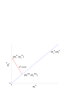
Figure 1: Sketch of the path (red, solid line) in the $(m_{l}^{\mbox{\tiny$R$}},m_{s}^{\mbox{\tiny$R$}})$ plane to the physical point $(m_{l}^{\mbox{\tiny$R$}\,*},m_{s}^{\mbox{\tiny$R$}\,*})$.

2 Theory

Our strategy is to start from a point with all $3$ sea quark masses equal,

$$m_{u}^{\mbox{\tiny$R$}}=m_{d}^{\mbox{\tiny$R$}}=m_{s}^{\mbox{\tiny$R$}}\equiv m_{0}^{\mbox{\tiny$R$}}\,,$$ (1)

and extrapolate towards the physical point, keeping the average sea quark mass

$$\overline{m}^{\mbox{\tiny$R$}}\equiv\mbox{\small$\frac{1}{3}$}(m_{u}^{\mbox{\tiny$R$}}+m_{d}^{\mbox{\tiny$R$}}+m_{s}^{\mbox{\tiny$R$}})$$ (2)

constant. For this trajectory to reach the physical point we have to start at a point where $m_{0}^{\mbox{\tiny$R$}}\approx\mbox{\small$\frac{1}{3}$}m_{s}^{\mbox{\tiny$R$}\,*}$. As we approach the physical point, the $u$ and $d$ quarks become lighter, but the $s$ becomes heavier. Pions are decreasing in mass, but $K$ and $\eta$ increase in mass as we approach the physical point.

We introduce the notation

$$\delta m_{q}^{\mbox{\tiny$R$}} \equiv m_{q}^{\mbox{\tiny$R$}}-\overline{m}^{\mbox{\tiny$R$}}\,,\qquad q=u,d,s\,,$$ (3)

and later use a similar notation for bare quark masses. (We will be mainly interested in the $2+1$ flavour case, with $m_{u}^{\mbox{\tiny$R$}}=m_{d}^{\mbox{\tiny$R$}}\equiv m_{l}^{\mbox{\tiny$R$}}$.) With this notation, the quark mass matrix is

$$\cal M = \left(\begin{array}[]{ccc}m_{u}^{\mbox{\tiny$R$}}&0&0\\ 0&m_{d}^{\mbox{\tiny$R$}}&0\\ 0&0&m_{s}^{\mbox{\tiny$R$}}\\ \end{array}\right)$$ (7)

$$= \overline{m}^{\mbox{\tiny$R$}}\left(\begin{array}[]{ccc}1&0&0\\ 0&1&0\\ 0&0&1\\ \end{array}\right)+\mbox{\small$\frac{1}{2}$}(\delta m_{u}^{\mbox{\tiny$R$}}-\delta m_{d}^{\mbox{\tiny$R$}})\left(\begin{array}[]{ccc}1&0&0\\ 0&-1&0\\ 0&0&0\\ \end{array}\right)+\mbox{\small$\frac{1}{2}$}\delta m_{s}^{\mbox{\tiny$R$}}\left(\begin{array}[]{ccc}-1&0&0\\ 0&-1&0\\ 0&0&2\\ \end{array}\right)\,.$$ (17)

The mass matrix ${\cal M}$ has a singlet part (proportional to $I$) and an octet part, proportional to $\lambda_{3}$, $\lambda_{8}$. In the $2+1$ case $\delta{m}_{u}^{\mbox{\tiny$R$}}=\delta{m}_{d}^{\mbox{\tiny$R$}}$ and isospin is a good symmetry. We argue that the theoretically cleanest way to approach the physical point is to keep the singlet part of ${\cal M}$ constant, and vary only the non-singlet parts. One technical advantage of this strategy is that it simplifies the quark mass renormalisation. In the case of clover/Wilson fermions, the singlet and non-singlet parts of the mass matrix will renormalise with different renormalisation constants [2]

$$m_{q}^{R}=Z_{m}^{NS}(m_{q}+\alpha_{Z}\overline{m})\,,\qquad\alpha_{Z}={Z_{m}^{\mbox{\tiny$S$}}-Z_{m}^{\mbox{\tiny$N\!S$}}\over Z_{m}^{\mbox{\tiny$N\!S$}}}\,,$$ (18)

where $\alpha_{Z}$ represents the fractional difference between the renormalisation constants. (Numerically this factor is $\sim O(1)$, and is thus non-negligible. Of course, for chiral fermions $\alpha_{Z}=0$.) This gives

$$\overline{m}^{\mbox{\tiny$R$}}=Z_{m}^{\mbox{\tiny$N\!S$}}(1+\alpha_{Z})\overline{m}\,,$$ (19)

and so by keeping the singlet mass constant we avoid the need to use two different $Z$s. This means that even for clover actions it does not matter whether we keep the bare or renormalised average sea quark mass constant (so we shall drop the ${}^{\mbox{\tiny$R$}}$ superscript in the following considerations).

An important advantage of our strategy is that it strongly constrains the possible mass dependence of physical quantities, and so simplifies the extrapolation towards the physical point. Consider a flavour singlet quantity (for example the scale $r_{0}$, or the plaquette $P$) at the symmetric point $(m_{0},m_{0},m_{0})$. If we make small changes in the quark masses, symmetry requires

$${\partial r_{0}\over\partial m_{u}}={\partial r_{0}\over\partial m_{d}}={\partial r_{0}\over\partial m_{s}}\,.$$ (20)

If we keep $m_{u}+m_{d}+m_{s}$ constant, $dm_{s}=-dm_{u}-dm_{d}=-2dm_{l}$ so

$$dr_{0}=dm_{u}\frac{\partial r_{0}}{\partial m_{u}}+dm_{d}\frac{\partial r_{0}}{\partial m_{d}}+dm_{s}\frac{\partial r_{0}}{\partial m_{s}}=0\,.$$ (21)

The effect of making the strange quark heavier exactly cancels the effect of making the light quarks lighter, so we know that $r_{0}$ must have be stationary at the symmetrical point. This makes extrapolations towards the physical point much easier, especially since we find that in practice quadratic terms in the quark mass expansion are very small. Any permutation of the quarks, such as an interchange $u\leftrightarrow s$, or a cyclic permutation $u\to d\to s\to u$ doesn’t change the physics, it just renames the quarks. Any quantity unchanged by all permutations will be flat at the symmetric point, like $r_{0}$. We can also construct permutation-symmetric combinations of hadrons. For example, for the decuplet, any permutation of the quark labels will leave the $\Sigma^{0*}$, ($uds$) unchanged, so the $\Sigma^{0*}$ is shown by a single black point in Fig. 2.

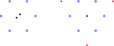
Figure 2: The behaviour of the octet and decuplet under the permutation group $S_{3}$. The colours denote sets of particles which are invariant under permutations of the quark flavours.

On the other hand, a permutation (such as $u\to d\to s$) can change a $\Delta^{++}(uuu)$ into a $\Delta^{-}(ddd)$ or (if repeated) into an $\Omega^{-}(sss)$, so these three particles form a set of baryons which is closed under quark permutations, and are all given the same colour (red) in Fig. 2. Finally the $6$ baryons consisting of two quarks of one flavour, and one quark of a different flavour, form an invariant set, shown in blue in Fig. 2. If we sum the masses in any of these sets, we get a flavour-symmetric quantity, which will obey the same argument we gave in eq. (21) for the quark mass (in)dependence of the scale $r_{0}$. We therefore expect that the $\Sigma^{0*}$ mass must be flat at the symmetric point, and furthermore that the combinations $(M_{\Delta^{++}}+M_{\Delta^{-}}+M_{\Omega})$ and $(M_{\Delta^{+}}+M_{\Delta^{0}}+M_{\Sigma^{*+}}+M_{\Sigma^{*-}}+M_{\Xi^{*0}}+M_{\Xi^{*-}})$ will also be flat. Technically these symmetrical combinations are in the $A_{1}$ singlet representation of the permutation group $S_{3}$. We list some of these invariant mass combinations in Table 1.

Decuplet	$2M_{\Delta}+M_{\Omega}$	red
baryons	$2(M_{\Delta}+M_{\Sigma^{*}}+M_{\Xi^{*}})$	blue
	$M_{\Sigma^{*}}$	black
Octet	$2(M_{N}+M_{\Sigma}+M_{\Xi})$	blue
baryons	$M_{\Sigma}+M_{\Lambda}$	black
Pseudoscalar	$4M_{K}^{2}+2M_{\pi}^{2}$	blue
mesons	$M^{2}_{\pi}+M^{2}_{\eta_{8}}$	black
Vector	$4M_{K^{*}}+2M_{\rho}$	blue
mesons	$2M_{\rho}+M_{\phi_{s}}$	black

Table 1: Permutation invariant mass combinations, see Fig. 2. $\phi_{s}$ is a fictitious $s\overline{s}$ particle; $\eta_{8}$ a pure octet meson. The colours in the third column correspond to Fig. 2.

We can use the singlet combinations from this table to locate the starting point of our path to physics by fixing a dimensionless ratio such as

$${X_{\pi}^{2}\over X_{N}^{2}}=\mbox{physical value}\,,$$ (22)

where $X_{\pi}^{2}=\mbox{\small$\frac{1}{3}$}(2M_{K}^{2}+M_{\pi}^{2})$ and $X_{N}=\mbox{\small$\frac{1}{3}$}(M_{N}+M_{\Sigma}+M_{\Xi})$. The permutation group $S_{3}$ yields a lot of useful relationships, but cannot capture the entire structure. For example, there is no way to make a connection between the $\Delta^{++}(uuu)$ and the $\Delta^{+}(uud)$ by permuting quarks. To go further, we need to classify physical quantities by $SU(3)$ and the permutation group $S_{3}$ (which is a subgroup of $SU(3)$).

Let us first consider linear terms in $\delta m_{q}$. These are given in Table 2.

Polynomial		$S_{3}$	$SU(3)$
$1$	✓	$A_{1}$	1
$(\overline{m}-m_{0})$		$A_{1}$	1
$\delta{m}_{s}$	✓	$E^{+}$		8
$(\delta{m}_{u}-\delta{m}_{d})$	✓	$E^{-}$		8
$(\overline{m}-m_{0})^{2}$		$A_{1}$	1
$(\overline{m}-m_{0})\delta{m}_{s}$		$E^{+}$		8
$(\overline{m}-m_{0})(\delta{m}_{u}-\delta{m}_{d})$		$E^{-}$		8
$\delta{m}_{u}^{2}+\delta{m}_{d}^{2}+\delta{m}_{s}^{2}$	✓	$A_{1}$	1		27
$3\delta{m}_{s}^{2}-(\delta{m}_{u}-\delta{m}_{d})^{2}$	✓	$E^{+}$		8	27
$\delta{m}_{s}(\delta{m}_{d}-\delta{m}_{u})$	✓	$E^{-}$		8	27

Table 2: All the quark-mass polynomials up to $O(m_{q}^{2})$, classified by symmetry properties. A tick (✓) marks the polynomials relevant on a constant $\overline{m}$ surface. These polynomials are plotted in Fig. 4.

Since we are keeping $\overline{m}$ constant, we are only changing the octet part of the mass matrix in eq. (17). Therefore, to first order in the mass change, only octet quantities can be effected. $SU(3)$ singlets have no linear dependence on the quark mass, as we have already seen by the symmetry argument eq. (21), but we now see that all quantities in $SU(3)$ multiplets higher than the octet cannot have linear terms. This provides a constraint on the hadron masses within a multiplet and leads to the Gell-Mann Okubo mass relations [4].

In the $2+1$ limit the decuplet baryons have $4$ different masses (for the $\Delta$, $\Sigma^{*}$, $\Xi^{*}$, and $\Omega$), but there is only one slope parameter in the linear mass formula. Similarly, for the octet baryons there are $4$ distinct masses, $(N,\Lambda,\Sigma,\Xi)$, but only $2$ slopes; and for octet mesons, one slope parameter for three mesons, ($\pi,K,\eta$). Mesons have fewer slope parameters than baryons because of constraints due to charge conjugation. In the meson octet the $K$ and $\overline{K}$ must have the same mass, but there is no reason why the $N$ and $\Xi$, (which occupy the corresponding places in the baryon octet), should have equal masses once flavour $SU(3)$ is broken.

When we proceed to quadratic polynomials we can construct polynomials which transform like mixtures of the $1$, $8$ and $27$ multiplets of $SU(3)$, Table 2. This covers all the structures that can arise in the octet mass matrix, but the decuplet mass matrix can include terms with the symmetries $10$, ${\overline{10}},$ and $64$, which first occur when we look at cubic polynomials in the quark masses, Table 3.

Polynomial		$S_{3}$	$SU(3)$
$(\overline{m}-m_{0})^{3}$		$A_{1}$	1
$(\overline{m}-m_{0})^{2}\delta{m}_{s}$		$E^{+}$		8
$(\overline{m}-m_{0})^{2}(\delta{m}_{u}-\delta{m}_{d})$		$E^{-}$		8
$(\overline{m}-m_{0})(\delta{m}_{u}^{2}+\delta{m}_{d}^{2}+\delta{m}_{s}^{2})$		$A_{1}$	1				27
$(\overline{m}-m_{0})\left[3\delta{m}_{s}^{2}-(\delta{m}_{u}-\delta{m}_{d})^{2}\right]$		$E^{+}$		8			27
$(\overline{m}-m_{0})\delta{m}_{s}(\delta{m}_{d}-\delta{m}_{u})$		$E^{-}$		8			27
$\delta{m}_{u}\delta{m}_{d}\delta{m}_{s}$	✓	$A_{1}$	1				27	64
$\delta{m}_{s}(\delta{m}_{u}^{2}+\delta{m}_{d}^{2}+\delta{m}_{s}^{2})$	✓	$E^{+}$		8			27	64
$(\delta{m}_{u}-\delta{m}_{d})(\delta{m}_{u}^{2}+\delta{m}_{d}^{2}+\delta{m}_{s}^{2})$	✓	$E^{-}$		8			27	64
$(\delta{m}_{s}-\delta{m}_{u})(\delta{m}_{s}-\delta{m}_{d})(\delta{m}_{u}-\delta{m}_{d})$	✓	$A_{2}$			10	$\overline{10}$		64

Table 3: The cubic quark-mass polynomials, classified by symmetry properties. A tick (✓) marks the polynomials relevant on a constant $\overline{m}$ surface. These polynomials are plotted in Fig. 4.

The allowed quark mass region on the $\overline{m}=\mbox{const.}$ surface is an equilateral triangle, as shown in Fig. 3.

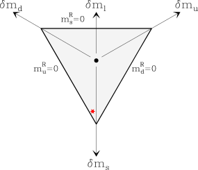
Figure 3: The allowed quark mass region on the $\overline{m}=\mbox{const.}$ surface is an equilateral triangle. The black point at the center is the symmetric point, the red star is the physical point. $2+1$ simulations lie on the vertical symmetry axis. The physical point is slightly off the $2+1$ axis because $m_{d}>m_{u}$.

Plotting the polynomials of Tables 2, 3 then gives the figures in Fig. 4, where the colour coding indicates whether the polynomial is positive (red) or negative (blue).

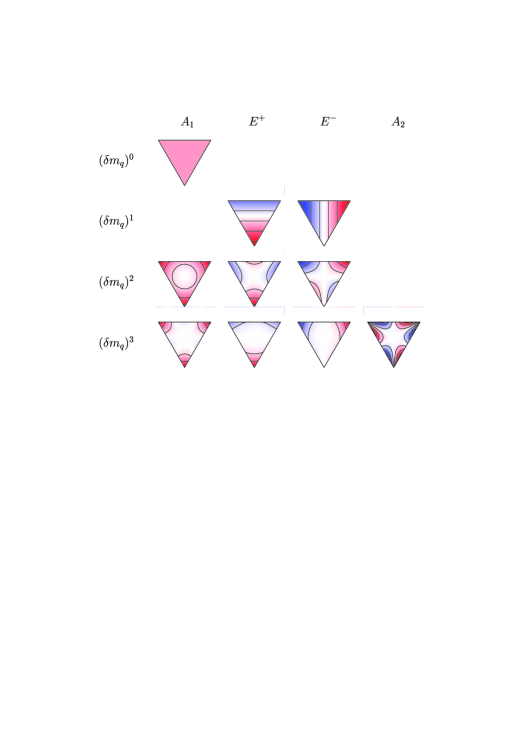
Figure 4: Contour plots of the polynomials relevant for the constant $\overline{m}$ Taylor expansion, see Tables 2, 3. A red(dish) colour denotes a positive number while a blue(ish) colour indicates a negative number. If $m_{u}=m_{d}$ (the $2+1$ case), only the polynomials in the $A_{1}$ and $E^{+}$ columns contribute.

We can see how well this works in practice by looking at the physical masses of the decuplet baryons,

$$4M_{\Delta}+3M_{\Sigma^{*}}+2M_{\Xi^{*}}+M_{\Omega} = 13.821{\rm\ GeV}\qquad\quad\ {\rm singlet}\quad\propto(\delta m_{l})^{0}$$

$$-2M_{\Delta}\qquad\ \quad+M_{\Xi^{*}}+M_{\Omega} = \ 0.742{\rm\ GeV}\qquad\quad\ {\rm octet}\qquad\propto(\delta m_{l})^{1}$$

$$4M_{\Delta}-5M_{\Sigma^{*}}-2M_{\Xi^{*}}+3M_{\Omega} = -0.044{\rm\ GeV}\qquad\quad{\rm 27plet}\qquad\propto(\delta m_{l})^{2}$$

$$-M_{\Delta}+3M_{\Sigma^{*}}-3M_{\Xi^{*}}+M_{\Omega} = -0.006{\rm\ GeV}\qquad\quad{\rm 64plet}\qquad\propto(\delta m_{l})^{3}\qquad\hbox{}$$ (23)

When we form combinations with particular $SU(3)$ symmetries we see a strong hierarchy, which suggests a short Taylor series may work well all the way from symmetry point $(m_{0},m_{0},m_{0})$ to the physical point. This gives the constrained fit formulae

$$M_{\pi}^{2} = M_{0}^{2}+2\alpha\delta m_{l}+(\beta_{0}+2\beta_{1})\delta m_{l}^{2}$$

$$M_{K}^{2} = M_{0}^{2}-\alpha\delta m_{l}+(\beta_{0}+5\beta_{1}+9\beta_{2})\delta m_{l}^{2}$$

$$M_{\eta_{s}}^{2} = M_{0}^{2}-4\alpha\delta m_{l}+(\beta_{0}+8\beta_{1})\delta m_{l}^{2}\,,$$ (24)

$$M_{\rho} = M_{0}+2\alpha\delta m_{l}+(\beta_{0}+2\beta_{1})\delta m_{l}^{2}$$

$$M_{K^{*}} = M_{0}-\alpha\delta m_{l}+(\beta_{0}+5\beta_{1}+9\beta_{2})\delta m_{l}^{2}$$

$$M_{\phi_{s}} = M_{0}-4\alpha\delta m_{l}+(\beta_{0}+8\beta_{1})\delta m_{l}^{2}\,,$$ (25)

$$M_{N} = M_{0}+3A_{1}\delta m_{l}+(B_{0}+3B_{1})\delta m_{l}^{2}$$

$$M_{\Lambda} = M_{0}+3A_{2}\delta m_{l}+(B_{0}+6B_{1}-3B_{2}+9B_{4})\delta m_{l}^{2}$$

$$M_{\Sigma} = M_{0}-3A_{2}\delta m_{l}+(B_{0}+6B_{1}+3B_{2}+9B_{3})\delta m_{l}^{2}$$

$$M_{\Xi} = M_{0}-3(A_{1}-A_{2})\delta m_{l}+(B_{0}+9B_{1}-3B_{2}+9B_{3})\delta m_{l}^{2}\,,$$ (26)

$$M_{\Delta} = M_{0}+3A\delta m_{l}+(B_{0}+3B_{1})\delta m_{l}^{2}$$

$$M_{\Sigma^{*}} = M_{0}+0+(B_{0}+6B_{1}+9B_{2})\delta m_{l}^{2}$$

$$M_{\Xi^{*}} = M_{0}-3A\delta m_{l}+(B_{0}+9B_{1}+9B_{2})\delta m_{l}^{2}$$

$$M_{\Omega} = M_{0}-6A\delta m_{l}+(B_{0}+12B_{1})\delta m_{l}^{2}\,.$$ (27)

While the linear terms are highly constrained, the quadratic terms much less so; indeed only for the baryon decuplet is there any constraint . Note also that for the pseudoscalar octet, $M_{\eta_{s}}$ is a fictitious $s\overline{s}$ particle (due to non-perfect $\eta$-$\eta^{\prime}$ mixing), while for the vector octet due to near perfect mixing between the $\phi$ and $\omega$ the $M_{\phi}$ is (almost) a perfect $s\overline{s}$ state, so that $M_{\phi_{s}}\approx M_{\phi}$. However even these fictitious particles still contain useful information, due to the constrained fit.

As eqs. (24)-(27) have been derived using only group theoretic arguments, then they will be valid for results derived on any lattice volume (though the coefficients are still functions of the volume).

What is the effect of higher order terms on our path in the $(m_{s},m_{l})$ plane? While at lowest order it did not matter whether we kept the quark mass constant or a particle mass now it does. Practically it is easiest to keep the (bare) quark mass fixed. Thus lines of constant $X_{S}$ are curved though they do still have to have the slope of $-2$ at the point where they cross the $SU(3)$ flavour symmetric line. Now we have to specify more closely what we mean when we keep $2m_{K}^{2}+m_{\pi}^{2}$ constant, as different scale choices give slightly different paths as sketched in Fig. 5.

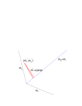
Figure 5: Sketch of some possible paths (red lines) in the $(m_{l},m_{s})$ plane to the physical point $(m_{l}^{\mbox{\tiny$R$}\,*},m_{s}^{\mbox{\tiny$R$}\,*})$.

Note that the physical domain $m_{l}^{\mbox{\tiny$R$}},m_{s}^{\mbox{\tiny$R$}}\geq 0$ translates to

$$m_{l}\geq-{\mbox{\small$\frac{1}{3}$}\alpha_{Z}\over(1+\mbox{\small$\frac{2}{3}$}\alpha_{Z})}m_{s}\,,\qquad m_{s} \geq -{\mbox{\small$\frac{2}{3}$}\alpha_{Z}\over(1+\mbox{\small$\frac{1}{3}$}\alpha_{Z})}m_{l}\,,$$ (28)

leading to non-orthogonal axes and possibly negative bare quark mass. (These features disappear for chiral fermions when $\alpha_{Z}=0$.) If we make different choices of the quantity we keep constant at the experimentally measured physical value, for example

$${X_{\pi}^{2}\over X_{N}^{2}}\,,\quad{X_{\pi}^{2}\over X_{\Delta}^{2}}\,,\quad{X_{\pi}^{2}\over X_{\rho}^{2}}\,,\quad{X_{\pi}^{2}\over X_{r}^{2}}\,,$$ (29)

where in addition to the previously defined singlet quantities we also now have $X_{\Delta}=\mbox{\small$\frac{1}{3}$}(2M_{\Delta}+M_{\Omega})$, $X_{\rho}=\mbox{\small$\frac{1}{3}$}(2M_{K^{*}}+M_{\rho})$, $X_{r}=r_{0}^{-1}$ we get slightly different trajectories. The different trajectories begin at slightly different points along the flavour $SU(3)$ symmetric line. Initially they are all parallel with slope $-2$, but away from the symmetry line they can curve, and will all meet at the physical point. (Numerically we shall later see that this seems to be a small effect.)

Finally we mention the connection of this method to $\chi$PT. For example for the pseudoscalar octet, using the results in [5] and assuming their validity up to the point on the flavour symmetric line, we find

$$M_{0}^{2} = \overline{\chi}\,\left[1-{16\overline{\chi}\over f_{0}^{2}}\left(3L_{4}+L_{5}-6L_{6}-2L_{8}\right)+{\overline{\chi}\over 24\pi^{2}f_{0}^{2}}\ln{\overline{\chi}\over\Lambda_{\chi}^{2}}\right]$$

$$\alpha = Q_{0}\,\left[1-{16\overline{\chi}\over f_{0}^{2}}\left(3L_{4}+2L_{5}-6L_{6}-4L_{8}\right)+{\overline{\chi}\over 8\pi^{2}f_{0}^{2}}\ln{\overline{\chi}\over\Lambda_{\chi}^{2}}\right]$$

$$\beta_{0} = -{Q_{0}^{2}\over 6\pi^{2}f_{0}^{2}}$$

$$\beta_{1} = {Q_{0}^{2}\over f_{0}^{2}}\,\left[-32\left(L_{5}-2L_{8}\right)+{1\over 24\pi^{2}}\left(7+4\ln{\overline{\chi}\over\Lambda_{\chi}^{2}}\right)\right]$$

$$\beta_{2} = {Q_{0}^{2}\over f_{0}^{2}}\,\left[16\left(L_{5}-2L_{8}\right)-{1\over 24\pi^{2}}\left(3+2\ln{\overline{\chi}\over\Lambda_{\chi}^{2}}\right)\right]\,,$$ (30)

with $Q_{0}=B_{0}^{\mbox{\tiny$R$}}Z_{m}^{\mbox{\tiny$N\!S$}}$, $\overline{\chi}=2Q_{0}(1+\alpha_{z})\overline{m}$, where the $L$s are appropriate Low Energy Constants or LECs. For clover fermions, as mentioned before we have to respect the fact that singlet and non-singlet quark masses renormalise differently which leads to a non-zero $\alpha_{Z}$.

We first note that when expanding the $\chi$-PT about a point on the $SU(3)$ flavour symmetry line gives to leading order only one parameter – $\alpha$. (This means, in particular, that flavour singlet combinations vanish to leading order, as discussed previously.) Secondly, while we fit to $\alpha$ and $\beta_{0}$, $\beta_{1}$ and $\beta_{2}$, it will be difficult to determine the individual LECs. The best we can probably hope for are these combinations.

3 The Lattice

We use a clover action for $2+1$ flavours with a single iterated mild stout smearing as described in [6]. Also given in this reference is a non-perturbative determination of the improvement coefficient for the clover term, using the Schrödinger Functional method. All the results given here will be at $\beta=5.50$, $c_{sw}=2.65$. HMC and RHMC were used for the $2$, $1$ fermion flavours respectively, [7], to generate the gauge configurations. The (bare) quark masses are defined as

$$am_{q}={1\over 2}\left({1\over\kappa_{q}}-{1\over\kappa_{sym;c}}\right)\,,$$ (31)

where vanishing of the quark mass along the $SU(3)$ flavour symmetric line determines $\kappa_{sym;c}$. We then keep $\overline{m}=\mbox{const.}\equiv m_{0}$ which gives

$$\kappa_{s}={1\over{{3\over\kappa_{sym}^{(0)}}-{2\over\kappa_{l}}}}\,.$$ (32)

So once we decide on $\kappa_{l}$ this then determines $\kappa_{s}$. A series of runs along the $SU(3)$ flavour line determines the initial point on this line: $\kappa_{sym}^{(0)}$ by looking when $X_{\pi}/X_{S}$, $S=N$, $\Delta$, $\rho$ are equal to their physical values, see eqs. (22), (29). This would also include $r$ if we have previously determined the physical value of $r_{0}$.

In Fig. 6 we plot $X_{\pi}^{2}/X_{S}^{2}$

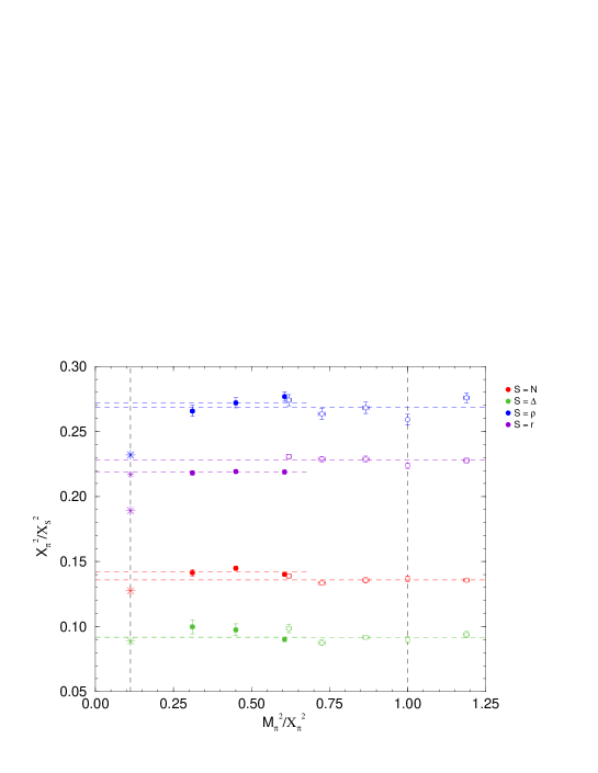
Figure 6: $X_{\pi}^{2}/X_{S}^{2}$ versus $M_{\pi}^{2}/X_{\pi}^{2}$ for $S=N$, $\Delta$, $\rho$, $r$ for $\kappa_{sym}^{(0)}=0.12090$. The dashed vertical line represents the physical value, while the dotted line gives the $SU(3)$ flavour symmetric point. Filled points are on $32^{3}\times 64$ lattices while open points are on $24^{3}\times 48$ sized lattice. Dashed horizontal lines represent constant fits to either the $32^{3}\times 64$ or $24^{3}\times 48$ results. The physical values are denoted by stars. For $r_{0}$ the small star is the value obtained using $r_{0}=0.5\,\mbox{fm}$ while the large star uses $r_{0}=0.467\,\mbox{fm}$ (determined for $n_{f}=2$ degenerate flavours [8]).

for various $X_{S}$ (with $S=N$, $\Delta$, $\rho$, $r$). Also shown are constant fits to the two volumes — $24^{3}\times 48$ and $32^{3}\times 64$. (The runs on $24^{3}\times 48$ lattices have $O(2000)$ trajectories, while the runs on $32^{3}\times 64$ lattices have $O(1500)$ trajectories.) As mentioned before we first simulate at various quark masses on the $SU(3)$ flavour symmetric line (i.e. $m_{\pi}^{2}/X_{\pi}^{2}=1$ in Fig. 6 where $\kappa_{sym}^{(0)}=0.12090$) to determine $\kappa_{sym}^{(0)}$. Note that simulations with a ‘light’ strange quark mass and heavy ‘light’ quark mass are possible – here the right most point. (In this inverted strange world we would expect $p\to\Sigma$ or $\Lambda$ decays.) It is apparent that while some scales fluctuate others (in particular $S=N$ and $r$) are very smooth. We take this as a sign that singlet quantities are very flat and the fluctuations are due to low statistics. Assuming that all ratios are constant, (i.e. higher order effects are small, see eq. (29)) we would expect all the ratios to converge to their experimental values. This is complicated because there are small finite size effects present (this can again best be seen in the $S=N$ and $r$ data). To investigate possible effects we are generating results on a variety of lattices, but for the present for the ratios we simply take the largest volume available. In Fig. 7

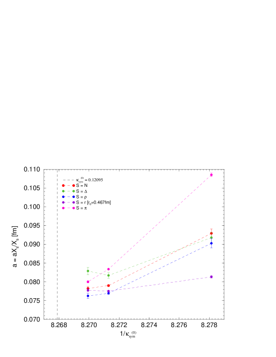
Figure 7: $aX_{S}/X_{S}$ against $1/\kappa^{(0)}_{sym}$ for $S=N$, $\Delta$, $\rho$, $r$, $\pi$ and $\kappa^{(0)}_{sym}=0.12080$, $0.12090$, $0.12092$. The vertical dashed line is at $\kappa^{(0)}_{sym}=0.12095$.

we plot $aX_{S}/X_{S}$, $S=N$, $\Delta$, $\rho$, $r$, $\pi$ for the largest volume fitted results from Fig. 6 (together with smaller data sets for $\kappa^{(0)}_{sym}=0.12080$, $\kappa^{(0)}_{sym}=0.12092$, the latter data set is presently only partially generated). This ratio gives estimates for the lattice spacing $a$ for the various scales. There appears to be convergence to a common scale of $a\sim 0.078\,\mbox{fm}$. To investigate this point further we are performing additional runs at $\kappa^{(0)}_{sym}=0.12092$ and $0.12095$.

4 Spectrum results

We now consider the mass spectrum. First we check whether there is a strong hierarchy due to the $SU(3)$ flavour symmetry as found in eq. (23). In Fig. 8

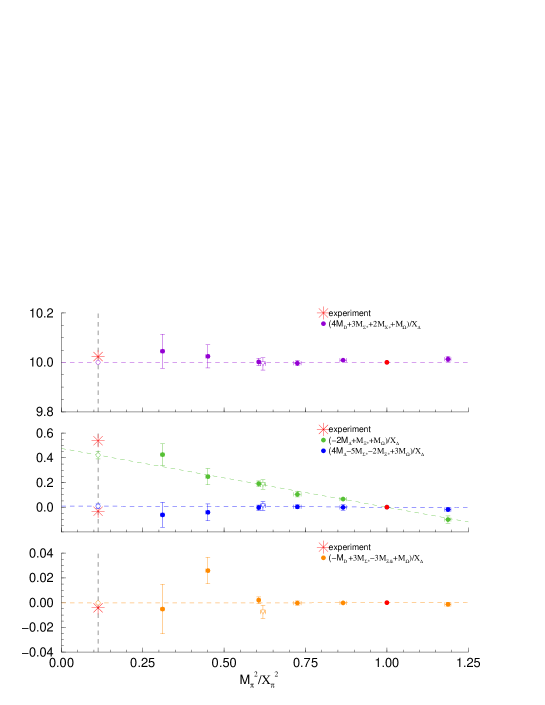
Figure 8: $(4M_{\Delta}+3M_{\Sigma^{*}}+2M_{\Xi^{*}}+M_{\Omega})/X_{\Delta}$, $(-2M_{\Delta}+M_{\Xi^{*}}+M_{\Omega})/X_{\Delta}$, $(4M_{\Delta}-5M_{\Sigma^{*}}-2M_{\Xi^{*}}+M_{\Omega})/X_{\Delta}$ and $(-M_{\Delta}+3M_{\Sigma^{*}}-3M_{\Xi^{*}}+M_{\Omega})/X_{\Delta}$ (filled circles) against $M_{\pi}^{2}/X_{\pi}^{2}$ together with a fit of constant, linear quadratic and cubic term in $\delta m_{l}$ respectively. Extrapolated values are shown as opaque circles. Experimental values are denoted by stars. The opaque triangle is a run at the same $(\kappa_{l},\kappa_{s})$, but on a $24^{3}\times 48$ lattice rather than a $32^{3}\times 64$ lattice.

we plot $(4M_{\Delta}+3m_{\Sigma^{*}}+2M_{\Xi^{*}}+M_{\Omega})/X_{\Delta}$, $(-2M_{\Delta}+M_{\Xi^{*}}+M_{\Omega})/X_{\Delta}$, $(4M_{\Delta}-5M_{\Sigma^{*}}-2M_{\Xi^{*}}+M_{\Omega})/X_{\Delta}$ and $(-M_{\Delta}+3M_{\Sigma^{*}}-3M_{\Xi^{*}}+M_{\Omega})/X_{\Delta}$ against $M_{\pi}^{2}/X_{\pi}^{2}$. Also shown are the experimental values. There is reasonable agreement with these numbers. (See [9] for a similar investigation of octet baryons.) It is also seen that as expected while $(-2M_{\Delta}+M_{\Xi^{*}}+M_{\Omega})/X_{\Delta}$ has a linear gradient in the pion mass, in the other fits any gradient is negligible. To check for possible finite size effects we also plot a run at the same $(\kappa_{l},\kappa_{s})$ but using $24^{3}\times 48$ lattice rather than $32^{3}\times 64$. There is little difference and so it appears that considering ratios of quantities within the same multiplet leads to (effective) cancellation of finite size effects.

In Fig. 9

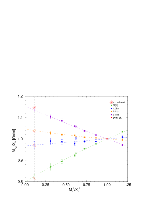
Figure 9: $M_{N_{O}}/X_{N}$ ($N_{O}=N$, $\Lambda$, $\Sigma$, $\Xi)$) against $M_{\pi}^{2}/X_{\pi}^{2}$ together with the combined fit of eqs. (26), (24) (the dashed lines). Experimental values are denoted by stars. The opaque triangle is a run at the same $(\kappa_{l},\kappa_{s})$, but on a $24^{3}\times 48$ lattice rather than a $32^{3}\times 64$ lattice.

we plot the nucleon octet $M_{N_{O}}/X_{N}$ (for $N_{O}=N$, $\Lambda$, $\Sigma$, $\Xi$) against $M_{\pi}^{2}/X_{\pi}^{2}$ for $\kappa_{sym}=0.12090$. A typical ‘fan’ structure is seen with results radiating from the common point on the symmetric line. Again, finite volume effects tend to cancel in the ratio (normalising with the singlet quantity from the same octet) and so both volumes have been used in the fit. The combined fit uses eqs. (26), (24) with the bare quark mass being an ‘internal’ parameter. Note that one point has a light strange quark and a heavy ‘light’ quark. Similarly in Figs. 10 and 11

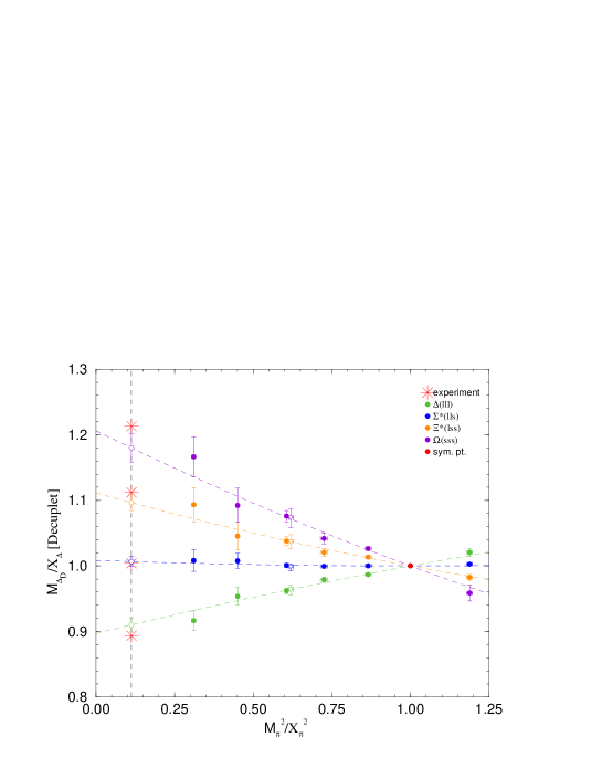
Figure 10: $M_{\Delta_{D}}/X_{\Delta}$ ($\Delta_{D}=\Delta$, $\Sigma^{*}$, $\Xi^{*}$, $\Omega$) against $M_{\pi}^{2}/X_{\pi}^{2}$ together with the combined fit of eqs. (27), (24). Same notation as Fig. 9.

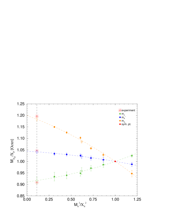
Figure 11: $M_{\rho_{O}}/X_{\rho}$ ($\rho_{O}=\rho$, $K^{*}$, $\phi_{s}$) against $M_{\pi}^{2}/X_{\pi}^{2}$ together with the combined fit of eqs. (25), (24) (the dashed lines). Same notation as Fig. 9.

we plot the corresponding nucleon decuplet $M_{\Delta_{D}}/X_{\Delta}$ and vector octet $M_{\rho_{O}}/X_{\rho}$ against $M_{\pi}^{2}/X_{\pi}^{2}$ respectively. Although we have included quadratic terms in the fit, there is really very little curvature in the results. We find good agreement with the experimental results.

5 Conclusions

We have outlined a programme to systematically approach the physical point starting from a point on the $SU(3)$ flavour symmetric line. Exploratory results for the hadron mass spectrum show that constrained linear extrapolations give accurate results for the mass spectrum. We are also applying this method to the computation of matrix elements, some initial results are given in [10, 11].

References

- [1] W. Bietenholz et al., [QCDSF–UKQCD Collaboration], Phys. Lett. B690, 436 (2010) [arXiv:1003.1114[hep-lat]].
- [2] M. Göckeler et al., [QCDSF–UKQCD Collaboration], Phys. Lett. B639, 307 (2006) [arXiv:hep-ph/0409312].
- [3] P. W. Atkins, M. S. Child and C. S. G. Phillips, “Tables for Group Theory”, (Oxford, 1970).
- [4] M. Gell-Mann, Phys. Rev. 125, 1067 (1962); S. Okubo, Prog. Theor. Phys. 27, 949 (1962).
- [5] C. Allton et al. [RBC–UKQCD Collaboration], Phys. Rev. D78, 114509 (2008) [arXiv:0804.0473[hep-lat]].
- [6] N. Cundy et al., [QCDSF–UKQCD Collaboration], Phys. Rev. D79, 094507 (2009) [arXiv:0901.3302[hep-lat]].
- [7] Y. Nakamura and H. Stüben, \posPoS(Lattice 2010)040.
- [8] A. Ali Khan et al., [QCDSF Collaboration], Phys. Rev. D74, 094508 (2006) [arXiv:hep-lat/0603028].
- [9] S. R. Beane et al., [NPLQCD Collaboration], Phys. Lett. B654, 20 (2007) [arXiv:hep-lat/0604013].
- [10] J. Zanotti et al., [QCDSF–UKQCD Collaboration], \posPoS(Lattice 2010)165.
- [11] F. Winter et al., [QCDSF–UKQCD Collaboration], \posPoS(Lattice 2010)163.
- [12] P. A. Boyle, Comp. Phys. Comm. 180, 2739 (2009).