Quark mass hierarchies in heterotic orbifold GUTs

Abstract

We discuss how to calculate Yukawa couplings in string-derived orbifold GUTs. As an application we investigate the quark mass hierarchies in these models. An interplay of different mechanisms derived from string theory leads to an interesting pattern. We discuss concrete examples in the context of heterotic orbifold compactifications.

1 Introduction

In the standard model (SM) of particle physics the structure of Yukawa couplings of quarks and leptons is completely undetermined. Yukawa couplings enter the model as free parameters. Adjusting these free parameters in an appropriate way, the theory is extremely successful in describing experimental results. Unfortunately it cannot explain the differences in the couplings and mixings. It would be appealing to explain all these input parameters like masses and mixings from a lower number of free parameters.

Heterotic string theory is one of the candidates for completing the SM in the ultraviolet. It was shown in the last years that heterotic orbifold compactifications can reproduce the particle content of the SM or its minimal supersymmetric version (MSSM) [1, 2]. Yukawa couplings are in these models no longer free parameters but depend on the size and the shape of the extra dimensions and the string coupling constant. It is possible to calculate the Yukawa couplings from first principles and compare them, as a test of the models, with the experimental data. If such a model is to describe the real world, it should reproduce the observed quark and lepton masses, CP phases and mixings. Recently it has been shown that it is possible to obtain the correct value for the top Yukawa coupling in these models quite naturally [3].

Motivated by this success this study is devoted to a calculation of the Yukawa couplings for the other particles. It is nearly impossible to calculate the couplings in string theory exactly due to the complexity of the calculations. Nevertheless the ratios between the couplings can be computed in a simple way. We will consider mainly tree-level effects, which means that we will ignore quantum corrections such as those coming from the renormalization group.

The comparison of the ratios between the different quark masses with the experimental data is quite exciting. We will show that the so-called benchmark models 1A and 1B [2] seem to be excluded due to their flavor structure. Maybe loop corrections induced through SUSY breaking [4] are able to break the obtained relations in the right way to get experimentally viable models.

In section 2 we will briefly introduce the mini-landscape models before we show in section 3 how we calculate the ratios between different couplings. In sections 4 and 5 we elaborate the flavor structure of the models 1A and 1B from [2] in more detail. Some technical details can be found in appendix A and B.

2 The mini-landscape models

In [2] several string derived models have been presented which are based on the so-called $\mathbbm{Z}_{6-\text{II}}$ heterotic orbifold compactification. It was shown that models with the exact MSSM spectrum with additional heavy vector-like exotics exist. These models have appealing phenomenological features like matter parity, a large top Yukawa coupling [3] and the possibility to include the seesaw mechanism to create neutrino masses [5]. The flavor structure of these models was also investigated in [6]. We will focus here on a specific example and show that the structure of the models is quite restrictive in a concrete example.

We focus on models which allow for a 6D orbifold GUT limit like the ones considered in [3] or [7]. Throughout this analysis we will assume that extra dimensions are compactified in such a way that this limit is realized. The geometry of the two extra dimensions is $\mathbbm{T}^{2}/\mathbbm{Z}_{2}$. The emerging extra dimensional structure is depicted in figure 1.

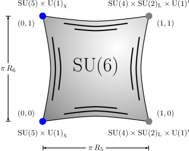
Figure 1: A 6D orbifold GUT. The fixed points are labeled with the two quantum numbers $(n_{2},n_{2}^{\prime})$. The first family sits at the fixed point labeled with $(0,1)$, the second family at the fixed point $(0,0)$. The third family and the Higgs fields live in the bulk.

The SM families are located at different points in the extra dimensions (see figure 1). These different location properties are not introduced by hand, but are a consequence of several string selection rules (see for example [8]). We will see that the flavor structure mainly depends on this localization. The fields are further localized in the additional four extra dimensions needed to have a consistent string theory. The influence on the flavor structure of these extra dimensions is subdominant as we will see in the next section. We can thus completely focus on the 6D GUT structure. A detailed discussion of the complete geometry can be found for example in [8].

3 Yukawa couplings in the heterotic mini-landscape

Yukawa couplings in the mini-landscape are not only 3-point functions, but are induced by higher order terms due to SM singlets. Let us discuss the origin of the Yukawa couplings in a concrete example. Consider the up type quark couplings

$$\mathcal{W}_{\text{Yukawa}}\supset Y_{u}^{ij}(R,\tilde{s})q_{i}\overline{u}_{j}\overline{\phi}_{1}$$ (3.1)

where $\tilde{s}$ denote standard model singlets, $R$ represents the dependence on the extra dimensions and the fields are labeled according to the notation in [2]. From a bottom-up perspective $Y_{u}^{ij}(R,\tilde{s})$ are free parameters which can be used to generate the observed quark masses. By contrast, in string theory these couplings are calculable. Matching string scattering amplitudes to the couplings in the corresponding low-energy field theory results in the schematic relation

$$Y_{u}^{ij}(R,\tilde{s})=\mathcal{A}_{u}^{ij}(R)\cdot\text{VEVs}$$ (3.2)

where $\mathcal{A}_{u}^{ij}(R)$ is the string scattering amplitude. The expression “VEVs” refers to the vacuum expectation value of SM singlets $\tilde{s}$ which induce this coupling. In general $Y_{u}^{ij}(R,\tilde{s})$ is a sum of several contributions (see for example equation (3.3)). $\mathcal{A}_{u}^{ij}(R)$ is the correlation function of string vertex operators on the string worldsheet which can be evaluated with the help of conformal field theory (CFT). It depends on the quantum numbers of the fields and especially on their origin in the extra dimensions.

Let us specifically consider the so-called benchmark model 1A of [2]. The Yukawa couplings for the first generation of up quarks are given by

$$\mathcal{A}_{u}^{11}=\left<q_{1}\overline{u}_{1}\overline{\phi}_{1}\cdot s^{0}_{4}s^{0}_{5}s^{0}_{26}\left(h_{1}h_{2}+s^{0}_{17}s^{0}_{18}+s^{0}_{20}s^{0}_{22}+s^{0}_{21}s^{0}_{22}+s^{0}_{20}s^{0}_{23}+s^{0}_{21}s^{0}_{23}\right)\right>$$ (3.3)

where $\overline{\phi}_{1}$ is the up type Higgs field and the additional fields are SM singlets $(\tilde{s})$. The brackets denote that we have to perform a CFT calculation to obtain a numerical value. The fields inside this correlator have to be understood as labels for the corresponding vertex operators on the string worldsheet. Because also the quarks and the Higgs field participate in this calculation we have included them in the above formulae. To avoid confusion we want to note that we use the same bracket notation for the VEV of a field as well as for string correlation functions. The value of the correlator (3.3) together with the VEVs of the singlets is then the model prediction for the coefficient $Y_{u}^{ij}(R,\tilde{s})$ given in equation (3.1). The singlet VEVs can be understood as expansion parameters of the superpotential.

The calculation can be performed using CFT techniques. The final result depends only on the localization of the fields in the extra dimensions. The reason why only the above outlined couplings are allowed are several string selection rules specified in detail in [8] and [2].

We want to explicitly calculate the above coupling in string theory in order to explain or at least motivate the hierarchy between the quark masses in the SM. The techniques to calculate such couplings in string theory have been developed long time ago [9, 10]. However, a technical obstruction to performing such a computation results from the fact that couplings in the heterotic mini-landscape are generated via SM singlets and we have to deal with higher order couplings. There are calculational tools available also for higher order couplings [11, 12, 13, 14], but it is difficult to obtain numerical quantities from these general results. Excited twist operators which appear through oscillator modes have not been considered in the literature for higher order couplings so far. These couplings occur frequently in the heterotic mini-landscape and it seems that we have to develop tools to address these couplings as well.

Before getting lost in a lot of technicalities it is worth to look at the structure of couplings first of all. We will see that it is not necessary to develop new tools, because the coupling structure is quite simple. As we shall see, the coupling strengths mainly depend on the location and on whether the fields have oscillator excitations. Table 1 shows the relevant data.

Particle	Twisted	Oscillator	$\tilde{N}^{*}_{f_{1}}$	$\tilde{N}^{*}_{f_{2}}$	$\tilde{N}^{*}_{f_{3}}$	$n_{3}$	$n_{2}$	$n_{2}^{\prime}$
$q_{1}$	$\checkmark$	-	-	-	-	0	0	1
$\overline{u}_{1}$	$\checkmark$	-	-	-	-	0	0	1
$\overline{\phi}_{1}$	-	-	-	-	-	$*$	$*$	$*$
$s^{0}_{4}$	$\checkmark$	$\checkmark$	-	1	-	0	0	0
$s^{0}_{5}$	$\checkmark$	$\checkmark$	1	-	-	0	0	0
$s^{0}_{26}$	$\checkmark$	$\checkmark$	-	1	-	0	$*$	$*$
$h_{1}$	$\checkmark$	-	-	-	-	0	$*$	$*$
$h_{2}$	$\checkmark$	-	-	-	-	0	$*$	$*$
$s^{0}_{17}$	$\checkmark$	-	-	-	-	0	$*$	$*$
$s^{0}_{18}$	$\checkmark$	-	-	-	-	0	$*$	$*$
$s^{0}_{20}$	$\checkmark$	-	-	-	-	1	$*$	$*$
$s^{0}_{21}$	$\checkmark$	-	-	-	-	1	$*$	$*$
$s^{0}_{22}$	$\checkmark$	-	-	-	-	2	$*$	$*$
$s^{0}_{23}$	$\checkmark$	-	-	-	-	2	$*$	$*$

Table 1: We show a set of relevant quantum numbers for some states of the model 1A. For the calculation of couplings the geometric origin and the oscillator numbers are highly important.

The notation is the same as in [2]. The six extra dimensions of the $\mathbbm{Z}_{6-\text{II}}$ orbifold compactification factorize in three two dimensional tori $\mathbbm{T}^{6}=\mathbbm{T}^{2}_{\text{G}_{2}}\times\mathbbm{T}^{2}_{\text{SU(3)}}\times\mathbbm{T}^{2}_{\text{SO(4)}}$. Each torus is described by a root lattice and an orbifold point group. As already mentioned we consider the limit in which the torus with the SO(4) root lattice and the $\mathbbm{Z}_{2}$ point group is large compared to the other four extra dimensions. The quantities $\tilde{N}^{*}_{f_{i}}$ indicate if a state is from the oscillator sector in the corresponding torus. Here $f_{1}$ refers to the $G_{2}$ torus, whereas $f_{2}$ labels the SU(3) torus and $f_{3}$ labels the SO(4) torus. The $G_{2}$ and SU(3) torus form four extra dimensions, whereas the SO(4) torus gives us the two additional extra dimensions depicted in figure 1. No state is an oscillator in the SO(4) torus which simplifies the calculation as we will see later on. The quantities $n_{2}$ and $n_{2}^{\prime}$ describe the localization in the SO(4) torus as already discussed and $n_{3}$ describes the localization in the SU(3) torus. A star ($*$) means that the state is a bulk field in this torus. The localization in the $G_{2}$ torus is not displayed in the table.

We can see that not all fields are twisted and not every field is an oscillator state. As already remarked, computing all involved correlators in string theory exactly will be painful. A useful strategy to get phenomenological interesting results has been examined for example in [3]. Computing a quantity exactly is often quite difficult, but the relation to another observable is sometimes very easy to obtain. We will use a similar strategy here. We do not calculate the Yukawa couplings exactly, but look at the ratios between them. As we can see by looking at the correlators in string theory, it is irrelevant where a term comes from, for example from a singlet or a quark. The only important point is where the fields are located. The reason for this behavior is of course that in heterotic string theory the different particles are just excitations of a closed string in ten dimensions. Because we are considering the interactions between closed strings we already incorporate all essential features. An additional advantage of this approach is that we do not have to take care about the Kähler potential because it is universal for the different couplings (see also [15]).

To be more concrete, let us take a look at another coupling. We find

$$\mathcal{A}_{u}^{12}=\left<q_{1}\overline{u}_{2}\overline{\phi}_{1}\cdot s^{0}_{4}s^{0}_{11}s^{0}_{26}\left(h_{1}h_{2}+s^{0}_{17}s^{0}_{18}+s^{0}_{20}s^{0}_{22}+s^{0}_{21}s^{0}_{22}+s^{0}_{20}s^{0}_{23}+s^{0}_{21}s^{0}_{23}\right)\right>.$$ (3.4)

The structure is the same as for the $Y_{u}^{11}$ coupling except for the fact that $s_{5}^{0}$ was interchanged by $s_{11}^{0}$. These singlets have the same quantum numbers (as can be seen in the appendix of [2]), but live at different fixed points (see also table 1). This is not an accident but a consequence of a $D_{4}$ symmetry [6]. The only difference between $\overline{u}_{1}$ and $\overline{u}_{2}$ is, that they also live at different fixed points. This means, that the interchange in the singlets just compensates the different location of the second family. We get

$$Y_{u}^{12}=\frac{\left<s_{11}^{0}\right>}{\left<s_{5}^{0}\right>}Y_{u}^{11}.$$ (3.5)

With $\left<\tilde{s}\right>$ we denote the vacuum expectation value (VEV) of a field $\tilde{s}$. We obtain similar relations like that, which only depend on the VEVs of some singlet fields and not on some difficult string theory calculation. Using these relations we can determine the structure of the Yukawa couplings in dependence of the yet unknown quantity $Y_{u}^{11}$.

4 The flavor structure of model 1A

4.1 The up quark sector

We will consider the up quark sector in the so-called benchmark model 1A in the heterotic mini-landscape in this section. In principle, this analysis can easily extended to all models in the mini-landscape. In [2] the couplings in the up quark sector were given by

$$Y_{u}=\begin{pmatrix}\tilde{s}^{5}&\tilde{s}^{5}&\tilde{s}^{5}\\ \tilde{s}^{5}&\tilde{s}^{5}&\tilde{s}^{6}\\ \tilde{s}^{6}&\tilde{s}^{6}&1\end{pmatrix}.$$ (4.1)

We have already looked in more detail at the couplings $Y_{u}^{11}$ and $Y_{u}^{12}$. The entry $Y_{u}^{33}$ was set to 1 because it already appears at the renormalizable level. In [3] it was shown that this coupling comes from the gauge coupling in the higher dimensional gauge theory and is slightly suppressed due to localization effects to fit in the right value. For our purposes we can just assume that the coupling to the top quark is of the right size and set it in the following to $y_{t}$.

We have collected the behavior of all necessary fields in table 1 and table 2.

Particle	Twisted	Oscillator	$\tilde{N}^{*}_{f_{1}}$	$\tilde{N}^{*}_{f_{2}}$	$\tilde{N}^{*}_{f_{3}}$	$n_{3}$	$n_{2}$	$n_{2}^{\prime}$
$q_{2}$	$\checkmark$	-	-	-	-	0	0	0
$\overline{u}_{2}$	$\checkmark$	-	-	-	-	0	0	0
$q_{3}$	-	-	-	-	-	$*$	$*$	$*$
$\overline{u}_{3}$	-	-	-	-	-	$*$	$*$	$*$
$s^{0}_{6}$	$\checkmark$	$\checkmark$	1	-	-	0	0	0
$s^{0}_{9}$	$\checkmark$	$\checkmark$	-	1	-	0	0	1
$s^{0}_{11}$	$\checkmark$	$\checkmark$	1	-	-	0	0	1

Table 2: More information on the participating fields in the up quark sector.

We start with a closer look at the coupling $Y_{u}^{11}$. As can be seen from the quantum numbers in table 1 the fields are located at different fixed points in the SO(4) torus depicted in figure 1. This different location will be encoded in the quantity $f(R_{6})$

$$Y_{u}^{11}=f(R_{6})A(\tilde{s}).$$ (4.2)

We will look at this quantity in more detail later (see also appendix A). We will see that the quark mass hierarchies are mainly controlled by $f(R_{6})$. The quantity $A(\tilde{s})$ is no longer depending on the localization of the fields in the SO(4) torus, but still on the localization in the other extra dimensions and on the singlet VEVs. The localization in the additional four extra dimensions will be irrelevant for our discussion and is therefore suppressed. The reason for that is that $A(\tilde{s})$ appears in every entry of $Y_{u}$ and can therefore not lead to a difference between the quark couplings.

Looking at the other couplings in detail we get

$$Y_{u}^{21}=Y_{u}^{12},\qquad Y_{u}^{22}=A(\tilde{s})$$ (4.3)

where we have taken the different localization of the second family in $Y_{u}^{22}$ into account. We have the same fields as for the $Y_{u}^{11}$ coupling despite the two quarks which are located at a different fixed point. For the $Y_{u}^{22}$ coupling all fields are located at the same fixed point in the SO(4) torus and we get no contribution from the localization in this torus. The coupling is completely insensitive to the volume of this torus.

When including also the third family things get more complicated. The third family is not localized and has its origin in the untwisted sector (see table 2). In order to obtain couplings to localized states, extra singlet VEVs are required, such that the couplings appear at higher order. We obtain for example

$$\begin{split}\mathcal{A}_{u}^{13}&=\left<q_{1}\overline{u}_{3}\overline{\phi}_{1}\cdot s^{0}_{4}s^{0}_{6}s^{0}_{11}s^{0}_{26}\left(h_{1}h_{2}+s^{0}_{17}s^{0}_{18}+s^{0}_{20}s^{0}_{22}+s^{0}_{21}s^{0}_{22}+s^{0}_{20}s^{0}_{23}+s^{0}_{21}s^{0}_{23}\right)\right>\\ &\quad+\left<q_{1}\overline{u}_{3}\overline{\phi}_{1}\cdot s_{13}^{0}\left(s^{0}_{4}s^{0}_{26}\right)^{2}\right>.\end{split}$$ (4.4)

Compared to $Y_{11}$ the singlet $s_{6}^{0}$ is here playing the role of $s_{5}^{0}$ whereas $s_{11}^{0}$ is playing the role of $\overline{u}_{1}$. Because $\overline{u}_{3}$ is from the untwisted sector it is irrelevant for our considerations. There is an additional term at order five in the singlets which we cannot easily relate to $Y_{u}^{11}$. We obtain

$$Y_{u}^{13}=\frac{\left<s_{6}^{0}\right>\left<s_{11}^{0}\right>}{\left<s_{5}^{0}\right>}Y_{u}^{11}+B(R_{6},\tilde{s}),\qquad Y_{u}^{31}=\left<s_{9}^{0}\right>Y_{u}^{11}$$ (4.5)

where $B(R_{6},\tilde{s})$ stands for an unknown contribution appearing at order five in the singlets. Furthermore we have

$$Y_{u}^{23}=\left<s_{6}^{0}\right>A(\tilde{s}),\qquad Y_{u}^{32}=\frac{\left<s_{9}^{0}\right>\left<s_{11}^{0}\right>}{\left<s_{5}^{0}\right>}Y_{u}^{11}.$$ (4.6)

The last term occurs already at the renormalizable level and we set it to $Y_{u}^{33}=y_{t}$ as already discussed. Putting everything together we get the matrix

$$Y_{u}=\begin{pmatrix}f(R_{6})A(\tilde{s})&\frac{\left<s_{11}^{0}\right>}{\left<s_{5}^{0}\right>}f(R_{6})A(\tilde{s})&\frac{\left<s_{6}^{0}\right>\left<s_{11}^{0}\right>}{\left<s_{5}^{0}\right>}f(R_{6})A(\tilde{s})+B(R_{6},\tilde{s})\\ \frac{\left<s_{11}^{0}\right>}{\left<s_{5}^{0}\right>}f(R_{6})A(\tilde{s})&A(\tilde{s})&\left<s_{6}^{0}\right>A(\tilde{s})\\ \left<s_{9}^{0}\right>f(R_{6})A(\tilde{s})&\frac{\left<s_{9}^{0}\right>\left<s_{11}^{0}\right>}{\left<s_{5}^{0}\right>}f(R_{6})A(\tilde{s})&y_{t}\end{pmatrix}.$$ (4.7)

This matrix contains several parameters. The singlet VEVs are, in principle, calculable as they are determined by F- and D-flatness constraints. However, in practice it is quite difficult to compute them. In what follows, we will see that one can nevertheless gain non-trivial information since we can understand the behavior of $f(R_{6})$ from a string theory calculation. Another important information is that the diagonal entries of $Y_{u}$ are completely independent of the VEVs. Let us now discuss the quantities $f(R_{6})$ and $B(R_{6},\tilde{s})$ in somewhat more detail.

The expression $f(R_{6})$ reflects the different localization of the first family in the SO(4) torus. It thus depends only on the moduli dependent part of the amplitude in this torus. We have four twisted fields and no oscillator. Looking at the location of the fields we can see that for $Y_{u}^{22}$ all fields live at the same fixed point in this torus. We conclude that there is no suppression due to instanton effects (see for example [9]). For $Y_{u}^{11}$ the situation changes. We get differently localized fields and thus an instanton suppression. As a first result we can assume that $Y_{u}^{22}\gg Y_{u}^{11}$ and therefore $f(R_{6})\ll 1$.

Whenever two fields from different fixed points interact the coupling is suppressed by the distance between the fields. If only fields from the same orbifold fixed point or from the bulk interact the coupling is unsuppressed.

A detailed look at a four twist calculation (as for example performed in [9]) tells us that the only difference between $Y_{u}^{11}$ and $Y_{u}^{22}$ is in the classical part of the amplitude. This is the instanton part which goes roughly like $e^{-R_{6}^{2}}$ where $\pi R_{6}$ is the distance between the two fixed points labeled with $n_{2}^{\prime}$ in the SO(4) torus (of course this distance is encoded in the $T$ modulus). We get the following suppression (see appendix A for a detailed calculation)

$$f(R_{6})=e^{-\frac{\pi R_{6}^{2}}{4}}.$$ (4.8)

The quantity $B(R_{6},\tilde{s})$ is quite difficult to discuss. It is a coupling involving six oscillators. It is also the only coupling depending on $s^{0}_{13}$. $B(R_{6},\tilde{s})$ appears only in one entry of the Yukawa matrix and thus it affects the result only marginaly.

Using this ingredients we can try to obtain quantitative results. The running of the couplings is neglected as it is beyond the accuracy of our approach (see also [3]). As a first test, the eigenvalues of $Y_{u}$ should give us the right ratio of the different up type quark masses. We start with fixed VEVs, all of the same size $\left<s^{0}_{i}\right>=0.1$. As usual we can change to mass eigenstates to relate the couplings in $Y_{u}$ to the quark masses. The diagonal entries of the rotated matrix have to be proportional to the quark masses. The experimental values are given in table 3.

Quark	Mass
up quark ($\overline{u}_{1}$)	$1.5-3.3\text{ MeV}$
charm quark ($\overline{u}_{2}$)	$1.27\begin{pmatrix}+0.07\\ -0.11\end{pmatrix}\text{ GeV}$
top quark ($\overline{u}_{3}$)	$171.3\pm 1.1\pm 1.2\text{ GeV}$

Table 3: Up quark masses from [16].

We get ratios between the quark masses like 500 between the first two generations and 100 between the second and the third generation

$$\frac{m_{u}}{m_{c}}\stackrel{{\scriptstyle!}}{{\approx}}\frac{1}{500},\qquad\frac{m_{c}}{m_{t}}\stackrel{{\scriptstyle!}}{{\approx}}\frac{1}{100}.$$ (4.9)

The impact of the VEVs and $B(R_{6},\tilde{s})$ is negligible and we ignore it. We therefore set $B(R_{6},\tilde{s})$ to zero.

The dependence on the remaining quantities is approximately given by

$$\frac{m_{u}}{m_{c}}\approx f(R_{6}),\qquad\frac{m_{c}}{m_{t}}\approx A(\tilde{s}).$$ (4.10)

If we choose $f(R_{6})=\frac{1}{500}$ we can get the right behavior with $A(\tilde{s})=\frac{1}{100}$. The off-diagonal terms are now quite small and we obtain the eigenvalues $m\approx(0.00002,0.01,1)$. Given the experimental values (displayed in table 3) these values are of the right size.

The small value of $f(R_{6})$ can be explained by the instanton suppression in the SO(4) torus. Using our result from equation (4.8) we obtain $R_{6}\approx 2.8$. As also remarked in [3] we expect to relate the distance $R_{5}$ between the two fixed points labeled by $n_{2}$ to the GUT scale, namely $M_{\text{GUT}}=\frac{1}{2R_{5}}$. As a starting point we use $R_{5}=50$, which gives us $M_{\text{GUT}}=\frac{1}{100}$ in Planck units. With these values we find an anisotropy of a factor of $\frac{R_{5}}{R_{6}}=18$ to get the right value for $R_{6}$. Given [3] such a value seems to be excluded. Nevertheless it is very encouraging that we get a value in the correct region. As outlined in section 4.2 the model suffers from more serious problems, therefore we do not address this point here in more detail. Another uncertainty is the value for $A(\tilde{s})$ which may or may not be realistic.

We conclude that even if we have a lot of unknowns, we can use the strong correlations between the couplings due to the different selection rules to make predictions. In contrast to the general analysis of [6] we find that the models are quite predictive. It is appealing that we have to consider in principle only a 6D GUT with differently localized families to explain the hierarchy for the up quark masses. We have obtained a very intuitive geometrical explanation and no miraculous string features at work. Taking the result of [3] into account the scenario is very constraint. We have one free parameter, namely $R_{6}$, to explain the ratio between the gauge coupling and the top Yukawa coupling and simultaneously the ratio between the up and the charm quark mass.

We proceed by looking at the remaining quark masses in the down quark sector.

4.2 The down quark sector

After the success of relating the quark masses in the up quark sector to the geometry of the extra dimensions, we will also try to explain the hierarchy for the down quark masses on the same footing. As we will see one cannot fit the up quark and the down quark masses simultaneously. The experimental data are displayed in table 4.

Quark	Mass
down quark ($\overline{d}_{1}$)	$3.5-6\text{ MeV}$
strange quark ($\overline{d}_{2}$)	$105\begin{pmatrix}+25\\ -35\end{pmatrix}\text{ MeV}$
bottom quark ($\overline{d}_{3}-\overline{d}_{4}$)	$4.2\begin{pmatrix}+0.17\\ -0.07\end{pmatrix}\text{ GeV}$

Table 4: Down quark masses from [16]. The labels for the quark masses are the same as in [2].

We find a mass ratio of 19 between the down and the strange quark mass [17] and a ratio around 40 between the strange and the bottom quark mass

$$\frac{m_{d}}{m_{s}}\stackrel{{\scriptstyle!}}{{\approx}}\frac{1}{19},\qquad\frac{m_{s}}{m_{b}}\stackrel{{\scriptstyle!}}{{\approx}}\frac{1}{40}.$$ (4.11)

We take into account couplings up to order nine in standard model singlets which correspond to 12-point couplings. Because we consider also couplings at higher order in singlets our starting point is slightly different from [2] and we start with

$$Y_{d}=\begin{pmatrix}\tilde{s}^{9}&\tilde{s}^{5}&0\\ \tilde{s}^{5}&\tilde{s}^{9}&0\\ 0&\tilde{s}^{6}&\tilde{s}^{8}\end{pmatrix}$$ (4.12)

which is a more accurate starting point. Repeating the steps of the discussion in the up quark sector we end up with a matrix like

$$Y_{d}=\begin{pmatrix}g_{1}(R_{6})C(\tilde{s})&f(R_{6})D(\tilde{s})&0\\ f(R_{6})D(\tilde{s})&g_{2}(R_{6})C(\tilde{s})&0\\ 0&X(R_{6},\tilde{s})&U(\tilde{s})\end{pmatrix}.$$ (4.13)

We have a lot of parameters, from a naive perspective it should be easily possible to fit the right values for all quark masses.

For the coupling between $q_{3}$ and the massless combination $\overline{d}_{3}-\overline{d}_{4}$ we find a coupling at order eight which is unsuppressed in the SO(4) torus because we find a coupling where all fields are localized at the same fixed point. Looking at the eigenvalues of the matrix we can see that the coupling $U(\tilde{s})$ exactly gives us one eigenvalue. As outlined above the coupling is not related to $R_{6}$ or $R_{5}$ and we can treat it as a free parameter to fit the bottom quark mass. The situation is similarly as for the top quark coupling, the third generation decouples from the first two generations.

For the other two quark masses the situation is more complicated. We find that $X(R_{6},\tilde{s})$ plays no role for the eigenvalues of $Y_{d}$ and is thus irrelevant for our discussion. The off-diagonal couplings $f(R_{6})D(\tilde{s})$ arise already at order five in standard model singlets and are suppressed in the SO(4) torus. We find the same factor as in the up quark sector, namely $f(R_{6})$ for the suppression. $f(R_{6})$ is the same as in the up quark sector, we have again four twisted fields in the SO(4) torus. Again two fields are localized at the fixed point labeled by $n_{2}^{\prime}=0$, whereas two of them are localized at the fixed point $n_{2}^{\prime}=1$. To be concrete, we obtain

$$\mathcal{A}_{d}^{12}=\left<q_{1}\overline{d}_{2}\phi_{1}\cdot s_{6}^{0}s_{9}^{0}s_{26}^{0}\left(h_{1}h_{2}+s^{0}_{17}s^{0}_{18}+s^{0}_{20}s^{0}_{22}+s^{0}_{21}s^{0}_{22}+s^{0}_{20}s^{0}_{23}+s^{0}_{21}s^{0}_{23}\right)\right>+\mathcal{O}(\tilde{s}^{6})$$ (4.14)

and thus

$$Y_{d}^{12}=f(R_{6})D(\tilde{s})=\frac{1}{\tan\beta}\frac{\left<s_{6}^{0}\right>\left<s_{9}^{0}\right>}{\left<s_{4}^{0}\right>\left<s_{5}^{0}\right>}Y_{u}^{11}+\mathcal{O}(\tilde{s}^{6}).$$ (4.15)

Inserting already the Higgs VEVs we can relate quantities from the up quark sector to the down quark sector. We have seen that $Y_{u}^{11}=f(R_{6})A(\tilde{s})$ together with $\tan\beta$ gives the up quark mass. We thus can see that $Y_{d}^{12}$ is of the right order to give us the down quark mass because the singlet VEVs are supposed to be of the same order of magnitude (see for example [18]). Of course, in detail the situation is more constrained, because $\tan\beta=1$ is excluded by experiments. An allowed value of about $\tan\beta>2$ [19] yields a too small down quark mass if the VEVs are of the same size. Nevertheless, this can be overcome due to an according VEV assignment. If this can be realistic or not is an open question.

We further note that we get contributions from higher order terms. These corrections do not affect the statement $Y_{d}^{12}=Y_{d}^{21}$ which is correct also up to order nine in the standard model singlets. The reason for this behavior is the $D_{4}$ symmetry [6].

The diagonal couplings $g_{1}(R_{6})C(\tilde{s})$ and $g_{2}(R_{6})C(\tilde{s})$ arise at order nine in standard model singlets. Their calculation is challenging. We have (for the quantum numbers of the additional fields see [2])

$$Y_{d}^{11}=g_{1}(R_{6})C(\tilde{s}),\qquad Y_{d}^{22}=\frac{g_{2}(R_{6})}{g_{1}(R_{6})}Y_{d}^{11}$$ (4.16)

with

$$\begin{split}\mathcal{A}_{d}^{11}&=\left<q_{1}\overline{d}_{1}\phi_{1}\cdot s_{4}^{0}\left(s_{13}^{0}\right)^{2}s_{26}^{0}s_{30}^{0}\big{(}\chi_{1}\chi_{2}h_{2}h_{4}+\chi_{3}\chi_{4}h_{2}h_{4}+\chi_{1}\chi_{4}h_{2}h_{6}+\chi_{2}\chi_{3}h_{2}h_{6}\right.\\ &\quad\left.+h_{2}h_{3}(h_{4})^{2}+h_{2}h_{3}(h_{6})^{2}+h_{2}h_{4}h_{5}h_{6}\right)\Big{>}.\end{split}$$ (4.17)

We find a similar behavior as in the up quark sector. The couplings for the first and second generation are not the same, but differ due to the different localization of the second family. We introduce the factors $g_{1}(R_{6})$ and $g_{2}(R_{6})$ which encode the localization behavior. We find for these couplings eight fields twisted in the SO(4) torus. There are always fields localized at different fixed points. We conclude that despite the fact that the coupling is already suppressed by a high power of singlet VEVs, the coupling is further suppressed due to the localization in the SO(4) torus (see also appendix B). Compared to the off-diagonal terms, these couplings are therefore rather small. We have to introduce two different factors because both couplings are suppressed. In the up quark case only the $Y_{u}^{11}$ coupling was suppressed.

We want to look at the eigenvalues to compare them to the experimental quark masses like in the up quark case. $X(R_{6},\tilde{s})$ is irrelevant for the eigenvalues due to the zeros in the matrix $Y_{d}$. Because the off-diagonal entries are identical and compared to the diagonal couplings quite large we get two almost degenerate eigenvalues. This is in contrast to data. To be more concrete we can estimate the difference between the couplings. If we assume rather large VEVs $\left<\tilde{s}\right>=0.3$ we get a suppression of $\left<\tilde{s}\right>^{4}\approx\frac{1}{125}$ between the diagonal and the off-diagonal couplings because the diagonal couplings arise at order nine and the off-diagonal couplings at order five in standard model singlets

$$C(\tilde{s})\approx\frac{1}{125}D(\tilde{s}).$$ (4.18)

We should point out that for smaller VEVs this ratio is even larger. If we use the results of appendix B we obtain

$$Y_{d}\approx\begin{pmatrix}\frac{1}{125}f(R_{6})D(\tilde{s})&f(R_{6})D(\tilde{s})&0\\ f(R_{6})D(\tilde{s})&\frac{1}{125}f(R_{6})D(\tilde{s})&0\\ 0&X(R_{6},\tilde{s})&U(\tilde{s})\end{pmatrix}.$$ (4.19)

We can tune $D(\tilde{s})$ to obtain the right ratio between the bottom and the strange quark mass regardless of $R_{6}$, but it is impossible to get a big ratio between the down and the strange quark mass. The quark mass ratios are

$$\frac{m_{d}}{m_{s}}\approx\frac{62}{63},\qquad\frac{m_{s}}{m_{b}}\approx\frac{126}{125}\frac{f(R_{6})D(\tilde{s})}{U(\tilde{s})}.$$ (4.20)

The mass eigenvalues for $m_{d}$ and $m_{s}$ are almost degenerate for all possible values of the free parameters.

We conclude that it is impossible to obtain a quark mass hierarchy as expected from experimental data with our setup.

It was first proposed in [4] to generate Yukawa couplings via loop effects through SUSY breaking soft terms. This can be a mechanism to cure the problem in the down quark sector. This mechanism leads also naturally to flavor changing neutral currents (FCNCs) which have to be compatible with experimental bounds (see for example [20] in the string theory context). If it is possible to fulfill these bounds in this class of models remains an open task for future work. Maybe there are also other mechanism which can give rise to essential corrections to the down quark masses in the right way.

5 A comment on model 1B

In [2] another vacuum configuration called model 1B was considered. This model has an unbroken $D_{4}$ family symmetry for the first two generations. The difference to model 1A is that the symmetry is not broken by the VEV assignment. The consequence is that all couplings for the first two generations are equal. As we have seen in the last section for the model 1A, such a behavior is in conflict with observations. It seems to be impossible for such configurations to get a big ratio between the masses as required by experiment without radiative quark mass generation already mentioned in the last section. We conclude that these configurations are rather unrealistic by construction.

6 Summary

We have developed tools to study the quark mass pattern in heterotic orbifold compactifications. Specifically we have studied the flavor structure in two examples of the mini-landscape, namely the so-called benchmark models 1A and 1B. We have seen that without any difficult string theory calculation we can obtain several interesting results because the couplings enjoy relations. We have linked the quark masses to the extra dimensions like already in [3] for the top quark coupling. We have also found some relations between the up quark and the down quark sector depending on $\tan\beta$. Our study shows that it is possible to obtain simple relations for the Yukawa couplings even in complex string-derived setups.

For the concrete models studied in our analysis we found that it is impossible to get the right masses in the down quark sector without including large radiative contributions through SUSY breaking. We do not know if this feature is universal for all models in the mini-landscape. What we can state is that it seems to be quite easy to disfavor models from the mini-landscape. Because we have not succeeded in obtaining the right quark mass pattern, we have not looked at the mixing, namely the CKM matrix or the mass pattern in the lepton sector. With the techniques outlined in this paper this is in principle also possible.

In [21] and [22] powerful tools have been developed to study the discrete symmetries between the string selection rules. Maybe it is possible to find better string theory models with these techniques.

Appendix A $\boldsymbol{N}$-point couplings for four $\boldsymbol{\mathbbm{Z}_{2}}$ twists

To obtain the quantity $f(R_{6})$ we need to calculate a $N$-point coupling with four $\mathbbm{Z}_{2}$ twists. The calculation of a 4-point coupling with four $\mathbbm{Z}_{2}$ twists has been calculated long time ago [9, 10]. Let us review here the result. There are two different contributions, one from the quantum part and one from the classical part. The first is insensitive to the localization of the fields, whereas the latter one is sensitive. Thus the quantity $f(R_{6})$ is only influenced by the classical part. The result for the classical part is [9]

$$Z_{\text{cl}}(x)=\sum e^{-S_{\text{cl}}(x)}=\sum_{n_{0},n_{1}\in\mathbbm{Z}}e^{-\frac{\pi R_{6}^{2}}{\operatorname{Im}\tau(x)}\left|n_{1}+n_{0}\tau(x)+\frac{1}{2}(\epsilon_{1}+\epsilon_{0}\tau(x))\right|^{2}}$$ (A.1)

where we have

$$\tau(x)=\frac{i\,{}_{2}F_{1}\left(\frac{1}{2},\frac{1}{2},1,1-x\right)}{{}_{2}F_{1}\left(\frac{1}{2},\frac{1}{2},1,x\right)}=\frac{i\,K(1-x)}{K(x)}$$ (A.2)

and $\epsilon_{i}$ labels the fixed point of the twist fields. With $K(x)$ we mean the complete elliptic integral of the first kind. $x$ can be interpreted as the position of one of the vertex operators on the sphere. It cannot be fixed by $\text{PSL}(2,\mathbbm{C})$ invariance and has to be weighted by an integral in the end. That means we have one free complex modulus of the Riemann surface describing the string interaction. We further have $\epsilon_{i}=0$ for the fixed point $(n_{2},n_{2}^{\prime})=(0,0)$ and $\epsilon_{i}=1$ for the fixed point $(n_{2},n_{2}^{\prime})=(0,1)$.

If all fields live at the same fixed point $\epsilon_{0}=\epsilon_{1}=0$ we get an unsuppressed amplitude because the exponential breaks down. If the fields are localized at different fixed points, for example $\epsilon_{0}=0$ and $\epsilon_{1}=1$ we get a suppression going with the distance squared $R_{6}^{2}$. The terms for $n_{i}\neq 0$ are further suppressed and come from states winding also around the torus. We can neglect their contribution for simplicity and obtain

$$Z_{\text{cl}}(x)\approx\begin{cases}1&\text{all fields live at the same fixed point}\\ e^{-\frac{\pi R_{6}^{2}}{4\operatorname{Im}\tau(x)}}&\text{fields live at different fixed points}\end{cases}.$$ (A.3)

This is the exact classical contribution in the SO(4) torus, because all other fields are untwisted in the SO(4) torus. We do not know the contribution in the other extra dimensions, namely the SU(3) and the $\text{G}_{2}$ torus in detail. We know that the additional contribution is depending on $x$. Because we have to integrate over $x$ in the end, we have to approximate the result.

Let us focus now on the $N$-point coupling in more detail. We have a $N$-point coupling and therefore $N$ vertex operator positions on the worldsheet. We can fix three of them by $\text{PSL}(2,\mathbbm{C})$ invariance. Over the remaining $N-3$ positions we should integrate. At least one of these vertex operators is twisted in the SO(4) torus and we called his position $x$ (in fact it is also possible that all vertex operators in the SO(4) torus are undetermined by $\text{PSL}(2,\mathbbm{C})$ invariance, but we will not consider this case here). The other vertex operators are untwisted in the SO(4) torus and we do not know their contribution exactly, but they depend on all $N-3$ variables. Their contribution is the same, regardless of their localization in the SO(4) torus. The complete contribution coming from this localization enters via equation (A.3). If we call the unknown part from the SU(3) and $\text{G}_{2}$ torus and the contributions not affected by the localization in the SO(4) torus $U(x,x_{2},\ldots x_{N-3})$ we get

$$\intop d^{2}x\intop d^{2}x_{2}\ldots\intop d^{2}x_{N-3}Z_{\text{cl}}(x)U(x,x_{2},\ldots x_{N-3})$$ (A.4)

for the complete amplitude. We can approximate the function $Z_{\text{cl}}(x)$ by setting $x=\frac{1}{2}$ which is motivated by the shape of the function (see figure 2).

\psfrag{rx}{\small{$\mathsf{\textsf{Re}(x)}$}}\psfrag{ix}{\small{$\mathsf{\textsf{Im}(x)}$}}\psfrag{S}{\small{$\mathsf{S_{\textsf{cl}}(x)}$}}\includegraphics[width=227.62204pt]{classhape}

Figure 2: The function $S_{\text{cl}}(x)$ for the values $\epsilon_{0}=0$, $\epsilon_{1}=1$ and $R_{6}=2$.

We obtain $\tau(x)=i$ for this choice. We get

$$\intop d^{2}x\intop d^{2}x_{2}\ldots\intop d^{2}x_{N-3}U(x,x_{2},\ldots x_{N-3})$$ (A.5)

if all fields live at the same fixed point and the coupling is unsuppressed. In the case where the fields are localized at different fixed points we get

$$e^{-\frac{\pi R_{6}^{2}}{4}}\intop d^{2}x\intop d^{2}x_{2}\ldots\intop d^{2}x_{N-3}U(x,x_{2},\ldots x_{N-3}).$$ (A.6)

We recognize that the integrals are now the same. We conclude that the required ratio between an suppressed and an unsuppressed coupling is

$$f(R_{6})=\frac{e^{-\frac{\pi R_{6}^{2}}{4}}\intop d^{2}x\intop d^{2}x_{2}\ldots\intop d^{2}x_{N-3}U(x,x_{2},\ldots x_{N-3})}{\intop d^{2}x\intop d^{2}x_{2}\ldots\intop d^{2}x_{N-3}U(x,x_{2},\ldots x_{N-3})}=e^{-\frac{\pi R_{6}^{2}}{4}}$$ (A.7)

in a first approximation. The uncertainty of this approach is of course substantial, because the function $U(x,x_{2},\ldots x_{N-3})$ is unknown.

Appendix B $\boldsymbol{N}$-point couplings for eight $\boldsymbol{\mathbbm{Z}_{2}}$ twists

The functions $g_{1}(R_{6})$ and $g_{2}(R_{6})$ can be determined by looking at $N$-point couplings with eight $\mathbbm{Z}_{2}$ twists. The computation of this amplitude is more complicated than the one reviewed in appendix A. General $\mathbbm{Z}_{2}$ twist amplitudes have been considered in several papers [12, 23, 24, 25, 26, 27], also because they are of interest in the context of spin operators. The beautiful mathematics of hyperelliptic Riemann surfaces needed for these computations can be found for example in [28]. The factors $g_{1}(R_{6})$ and $g_{2}(R_{6})$ are not only given by the classical part of the amplitude, which is now depending on at least five free moduli of the Riemann surface $x_{1},\ldots x_{5}$. The reason for this is that different fields appear for different couplings and the quantum part is depending on all of these fields. Because our approach contains already a big uncertainty we assume

$$Z_{\text{qu}}=\mathcal{O}(1)$$ (B.1)

and neglect the quantum part for the following discussion. This can be justified due to the discussion in [29] in the context of magnetized brane models and will be discussed in more detail for heterotic orbifolds elsewhere.

The classical part can be written as

$$Z_{\text{cl}}=\sum e^{-S_{\text{cl}}(x_{1},\ldots,x_{5})}.$$ (B.2)

The dependence on $R_{6}$ is the same as for $f(R_{6})$. We find

$$g_{i}(R_{6})=e^{-\alpha_{i}R_{6}^{2}}$$ (B.3)

and thus again an exponential suppression of the order of $f(R_{6})$. The constants $\alpha_{i}>0$ are depending on the period matrix of the Riemann surface and on the integral approximation. The coupling $g_{1}(R_{6})$ is dominated by couplings where six twist fields are localized at one fixed point and two twist fields at the other fixed point. We thus conclude that $g_{1}(R_{6})\approx f(R_{6})$ (see for example [12]). For the coupling $g_{2}(R_{6})$ the dominant contribution originates from the same coupling as for the $g_{1}(R_{6})$ term. There is an additional contribution where four twist fields sit at one fixed point and four twist fields at the other fixed point. Nevertheless, this contribution is stronger suppressed [12]. We thus conclude that $g_{2}(R_{6})\approx g_{1}(R_{6})$. There is only a mild difference between $g_{2}(R_{6})$ and $g_{1}(R_{6})$ which we will neglect. For the numerical discussion of couplings we assume

$$g_{1}(R_{6})\approx g_{2}(R_{6})\approx f(R_{6}).$$ (B.4)

The error of this approximation is larger as for the calculation of $f(R_{6})$ discussed in appendix A.

References

- [1] W. Buchmüller, K. Hamaguchi, O. Lebedev, and M. Ratz, Phys. Rev. Lett. 96 (2006), 121602, [hep-ph/0511035].
- [2] O. Lebedev et al., Phys. Rev. D77 (2008), 046013, [0708.2691].
- [3] P. Hosteins, R. Kappl, M. Ratz, and K. Schmidt-Hoberg, JHEP 07 (2009), 029, [0905.3323].
- [4] W. Buchmüller and D. Wyler, Phys. Lett. B121 (1983), 321.
- [5] W. Buchmüller, K. Hamaguchi, O. Lebedev, S. Ramos-Sánchez, and M. Ratz, Phys. Rev. Lett. 99 (2007), 021601, [hep-ph/0703078].
- [6] P. Ko, T. Kobayashi, J.-h. Park, and S. Raby, Phys. Rev. D76 (2007), 035005, [0704.2807].
- [7] W. Buchmüller, C. Lüdeling, and J. Schmidt, JHEP 09 (2007), 113, [0707.1651].
- [8] W. Buchmüller, K. Hamaguchi, O. Lebedev, and M. Ratz, Nucl. Phys. B785 (2007), 149–209, [hep-th/0606187].
- [9] L. J. Dixon, D. Friedan, E. J. Martinec, and S. H. Shenker, Nucl. Phys. B282 (1987), 13–73.
- [10] S. Hamidi and C. Vafa, Nucl. Phys. B279 (1987), 465.
- [11] S. A. Abel and A. W. Owen, Nucl. Phys. B682 (2004), 183–216, [hep-th/0310257].
- [12] J. J. Atick, L. J. Dixon, P. A. Griffin, and D. Nemeschansky, Nucl. Phys. B298 (1988), 1–35.
- [13] M. Bershadsky and A. Radul, Int. J. Mod. Phys. A2 (1987), 165–178.
- [14] K.-S. Choi and T. Kobayashi, Nucl. Phys. B797 (2008), 295–321, [0711.4894].
- [15] L. E. Ibanez and D. Lust, Nucl. Phys. B382 (1992), 305–364, [hep-th/9202046].
- [16] Particle Data Group, C. Amsler et al., Phys. Lett. B667 (2008), 1.
- [17] H. Leutwyler, Phys. Lett. B378 (1996), 313–318, [hep-ph/9602366].
- [18] R. Kappl et al., Phys. Rev. Lett. 102 (2009), 121602, [0812.2120].
- [19] G. Degrassi, S. Heinemeyer, W. Hollik, P. Slavich, and G. Weiglein, Eur. Phys. J. C28 (2003), 133–143, [hep-ph/0212020].
- [20] T. Banks, Nucl. Phys. B303 (1988), 172.
- [21] W. Buchmüller and J. Schmidt, Nucl. Phys. B807 (2009), 265–289, [0807.1046].
- [22] B. Petersen, M. Ratz, and R. Schieren, JHEP 08 (2009), 111, [0907.4049].
- [23] L. Alvarez-Gaume, G. W. Moore, and C. Vafa, Commun. Math. Phys. 106 (1986), 1–40.
- [24] R. Dijkgraaf, E. P. Verlinde, and H. L. Verlinde, Commun. Math. Phys. 115 (1988), 649–690.
- [25] V. G. Knizhnik, Commun. Math. Phys. 112 (1987), 567–590.
- [26] K. Miki, Phys. Lett. B191 (1987), 127.
- [27] A. B. Zamolodchikov, Nucl. Phys. B285 (1987), 481–503.
- [28] H. M. Farkas and I. Kra, Riemann surfaces, 2. ed., Springer Verlag, 1992.
- [29] H. Abe, K.-S. Choi, T. Kobayashi, and H. Ohki, JHEP 06 (2009), 080, [0903.3800].