Hydrodynamic modeling of deconfinement phase transition in nuclear collisions

Abstract

The (3+1)–dimensional ideal hydrodynamics is used to simulate collisions of gold nuclei with bombarding energies from 1 to 160 GeV per nucleon. The initial state is represented by two cold Lorentz-boosted nuclei. Two equations of state: with and without the deconfinement phase transition are used. We have investigated dynamical trajectories of compressed baryon-rich matter as functions of various thermodynamical variables. The parameters of collective flow and hadronic spectra are calculated. It is shown that presence of the deconfinement phase transition leads to increase of the elliptic flow and to flattening of proton rapidity distributions.

I Introduction

Relativistic hydrodynamics is a very popular approach to describe high–energy nuclear collisions. Especially useful is its sensitivity to the equation of state (EoS) of strongly interacting matter and, in particular, to its phase transitions. In fact, extracting this EoS is the main goal of heavy–ion experiments. Some signatures of a deconfined quark-gluon plasma (QGP) have been already found in RHIC experiments with c.m. bombarding energies $\sqrt{s_{NN}}=60-200$ GeV. Presumably, this plasma can be also created at lower (SPS, AGS) energies. A more detailed data should be obtained in the low–energy runs at RHIC and future FAIR and NICA experiments.

A large amount of experimental data on nuclear collisions at AGS, SPS and RHIC energies have been successfully described by different versions of the hydrodynamic model. The first model of this kind has been proposed by Landau Lan53 . One can roughly divide the existing versions of ideal hydrodynamics into two classes. The first class includes the models which apply fluid dynamical simulations from the very beginning, i.e. starting from cold equilibrium nuclei. The models of the second class introduce an excited and compressed initial state – a locally equilibrated ”fireball” formed at an early non-equilibrium stage of the collision. Up to now many versions of the fireball–based hydrodynamic model were developed ranging from simplified (1+1)– and (2+1)–dimensional models to more sophisticated (3+1)–dimensional ones (see  Sat07 and references therein).

Historically, early 3D hydrodynamic models of relativistic nuclear collisions Ams75 ; Sto79 used cold Lorentz-contracted nuclei in the initial state. However, such models become less justified at high bombarding energy due to the nuclear transparency effects.

One should have in mind that the hydrodynamical approach can not be directly applied to late stages of a heavy–ion reaction when binary collisions of particles become too rare to maintain the local thermodynamic equilibrium. A usual way Coo74 to circumvent this difficulty to introduce a so called ”freeze–out” criterium to stop the hydrodynamic description at late times. A more consistent procedure has been proposed in Refs. Bas00 ; Pet08 within a hybrid ”hydro–cascade” model.

In this paper we formulate a version of the ideal (3+1)–dimensional hydrodynamics suitable for the domain of NICA–FAIR energies. This model belongs to the first class and uses a new EoS Sat09 with the deconfinement and liquid–gas phase transitions. By performing simulations with and without the deconfinement phase transition we try to find the observables which are sensitive to creation of the QGP. A more detailed description of the results will be given in Ref. Mer10 .

II Formulation of the model

Below we study the evolution of highly excited, and possibly deconfined, strongly–interacting matter produced in ultrarelativistic heavy-ion collisions. It is assumed that this evolution can be described by the equations of ideal relativistic hydrodynamics Lan87 :

$$\partial_{\nu}T^{\mu\nu}=0\hskip 1.0pt,$$ (1)

$$\partial_{\mu}(nu^{\mu})=0\hskip 1.0pt.$$ (2)

Here $T^{\mu\nu}$ is energy-momentum tensor ($\hbar=c=1$)

$$T^{\mu\nu}=(\varepsilon+P)\hskip 1.0ptu^{\mu}u^{\nu}-P\hskip 1.0ptg^{\hskip 1.0pt\mu\nu},$$ (3)

$\varepsilon,n$ and $P$ are the rest–frame energy density, the net baryon density and pressure of the fluid, $u^{\mu}=(\gamma,\gamma\hskip 1.0pt\bm{v})^{\hskip 1.0pt\mu}$ is its collective 4–velocity, $\gamma=(1-\bm{v}^{2})^{-1/2}$, $\bm{v}$ is the fluid 3–velocity, $g^{\hskip 1.0pt\mu\nu}$ is the metric tensor. To solve Eqs. (1)–(3) it is necessary to specify the EoS $P=P(n,\varepsilon)$ of the fluid and initial conditions.

In our calculations we use the EoS of strongly interacting matter with the first order deconfinement phase transition (EoS–PT) Sat09 . The hadronic phase is described as the hadron resonance gas including known hadrons with masses up to 2 GeV. Finite size effects are taken into account by introducing the excluded volume corrections. The same excluded volume parameter $v_{e}=1$ fm³ is used for all hadronic species. A Skyrme–like mean field $U=U(n)$ is added to guarantee that the hadronic matter has correct saturation point and the liquid-gas phase transition. The quark–gluon phase is described by the bag model with lowest-order perturbative corrections. The phase transition boundaries and characteristics of the mixed phase (MP) are found by using the Gibbs conditions with the strangeness neutrality constraint.

To probe sensitivity to the EoS, we have also performed calculations with the EoS of ideal hadron gas (EoS–HG). In this case we disregard the excluded volume effects assuming that $v_{e}=0$. To provide stability of initial nuclei we also introduce the Skyrme-like mean field. The parameters of EoS–PT and EoS–HG are given in Ref. Sat09 . Our analysis shows that although generally the EoS with the phase transition is softer than the EoS of pure hadron gas, in some regions of thermodynamic parameters the EoS-PT has sound velocities of the same order or even larger than those in the EoS–HG.

Below we consider collisions of gold nuclei. The hydrodynamic simulation is started at the stage when two cold Lorentz-contracted nuclei approach each other. The initial baryon and energy density profiles of each nucleus in its rest frame are described by the Woods-Saxon distribution. Due to the stabilizing effect of the Skyrme-like mean field, the initial nuclei may stay in equilibrium with vacuum at $P=0$ . They propagate without distortion until their density distributions essentially overlap.

Below the beam axis is denoted by $z$ and the $x$–axis is chosen along the impact parameter vector $\bm{b}$. In our simulations we use linear interpolation of tables $P(n,\varepsilon)$ prepared with fixed steps in $\varepsilon$ and $n$. Analogous tables for temperature ($T$), baryon ($\mu$) and strange ($\mu_{S}$) chemical potentials are used for calculating hadronic spectra. The numerical solution of fluid–dynamical equations is obtained by using the relativistic version of the flux-corrected transport algorithm Bor73 .

To calculate hadronic momentum distributions we apply the approximation of instantaneous freeze-out: it is assumed that a sudden transition from the local equilibrium to collisionless propagation of particles takes place at some isochronous hypersurface ($t=t_{\rm fr}={\rm const}$). Within this approximation one can use the following formula Coo74 for the invariant momentum distribution of the hadronic species $i$

$$E\hskip 1.0pt\frac{d^{\hskip 1.0pt3}N_{i}}{d^{\hskip 1.0pt3}p}=\frac{d^{\hskip 1.0pt3}N_{i}}{dy\hskip 1.0ptd^{\hskip 1.0pt2}p_{\hskip 1.0ptT}}=\frac{g_{i}E}{(2\pi)^{\hskip 1.0pt3}}\int dV\left\{\exp\left(\frac{p_{\nu}u^{\nu}-\mu_{i}}{T}\right)\pm 1\right\}^{-1},$$ (4)

where $p^{\hskip 1.0pt\mu}=(E,\bm{p})^{\mu}$ is the 4–momentum of the particle, $y$ and $\bm{p}_{\hskip 1.0ptT}$ are, respectively, its longitudinal rapidity and transverse momentum, $g_{i}$ is the statistical weight of i-th hadrons. Plus and minus in Eq. (4) correspond, respectively, to fermions and bosons. Using conditions of chemical equilibrium one can express the particle’s chemical potential $\mu_{i}$ through the baryon and strange chemical potentials as follows

$$\mu_{i}=B_{i}\mu+S_{i}\mu_{S}\,,$$ (5)

where $B_{i}$ and $S_{i}$ are, respectively, the baryon and strangeness number of species $i$ .

In addition to contributions of ”thermal” nucleons and pions, which are calculated directly by using Eqs. (4)–(5), we also take into account resonance decays, e.g. $\Delta\to N\pi$, $\rho\to 2\pi$,…We use the standard formulae for two-body decays of resonances in the zero width approximation (the decays into more than two hadrons are treated approximately Sat07 ). All known resonances with masses up to 2 GeV are taken into account.

The transverse collective flows of matter created in heavy–ion collisions, are rather sensitive to the EoS. Especially useful is the elliptic flow characterized by the parameter $v_{2}$ Oll92 . To discuss qualitatively possible differences between the EoS–PT and EoS–HG, below we calculate the so–called momentum anisotropy parameter $\epsilon_{p}$ which characterizes the flow asymmetry in the azimuthal plane. Following Ref. Boz09 we define this quantity as

$$\epsilon_{p}=\frac{\displaystyle\int dx\hskip 1.0ptdy\left(T^{\hskip 1.0ptxx}-T^{\hskip 1.0ptyy}\right)}{\displaystyle\int dx\hskip 1.0ptdy\left(T^{\hskip 1.0ptxx}+T^{\hskip 1.0ptyy}\right)}\,,$$ (6)

where $T^{\hskip 1.0ptxx},T^{\hskip 1.0ptyy}$ are the components of the energy-momentum tensor in the azimuthal plane $z=0$. The approximate relation $\epsilon_{p}\simeq 2\hskip 1.0ptv_{2}$ has been obtained in Ref. Kol00 from (2+1)–hydrodynamical simulations of Pb+Pb collisions at SPS and RHIC energies.

III Results

First, let us discuss thermodynamic characteristics of matter created in relativistic Au+Au collisions. Our goal is to find differences between the results obtained with EoS–HG and EoS–PT. Figures 1–2 represent dynamical trajectories of matter in the central box ($|x|,\,|y|,\,|z|/\gamma_{0}\,<\,1\,{\rm fm}$) produced in central (b=0) Au+Au collisions at different bombarding energies $E_{\rm\hskip 1.0ptlab}$. Shown are the results for $n-\varepsilon$ and $\mu-T$ planes. At $E_{\rm\hskip 1.0ptlab}\gtrsim 5$ AGeV the calculation with EoS–PT predicts larger values of $\varepsilon$ and $n$ as compared to EoS–HG. In this case one can also see longer life-times of states with maximal compression and delay in transition to expansion stages. Note that calculations with EoS–PT predict a zigzag-like behavior of the trajectories in the $\mu-T$ plane with slightly raising temperature in the MP as a function of time. It is important to note that the final states of hadronic matter in the central cell are very similar for two EoS used in the calculations. In other words, all differences in the early dynamics are practically washed out in the final stage.

According to our analysis, especially interesting is the region of bombarding energies around $E_{\rm\hskip 1.0ptlab}\sim 10$ AGeV. At such energies we find an enhanced sensitivity of collective flows and particle spectra to the phase transition. Figure 3 represents the time evolution of the momentum anisotropy $\epsilon_{p}$ in semicentral Au+Au collisions at different $E_{\rm\hskip 1.0ptlab}$ . One can see that the momentum anisotropy is rather sensitive to EoS at $E_{\rm\hskip 1.0ptlab}\lesssim 20$ AGeV. The asymptotic values of $\epsilon_{p}$ at $E_{\rm\hskip 1.0ptlab}\gtrsim 10$ AGeV are larger in calculations with the deconfinement phase transition. This agrees with the similar conclusion of Ref. Pet10 .

To estimate sensitivity of these results to the choice of the freeze-out time, we determine the time moment when the energy density in a central box becomes smaller than a certain freeze-out value $\varepsilon_{\rm fr}$. In Fig. 3 we mark the values of $\epsilon_{p}$ corresponding to different values of $\varepsilon_{\rm fr}$. Figure 4 shows our results for the excitation function $\epsilon_{p}(E_{\rm\hskip 1.0ptlab})$. The lines connect the values $\epsilon_{p}$ taken at freeze-out times corresponding to $\varepsilon_{\rm fr}=0.4$ GeV/fm³. In the case of EoS–PT we predict a non-monotonic dependence of $\epsilon_{p}(E_{\rm\hskip 1.0ptlab})$ with maximum at $E_{\rm\hskip 1.0ptlab}\simeq 10$ AGeV. On the other hand, the existing experimental data on the elliptic flow in Au+Au and Pb+Pb collisions at AGS and low SPS energies do not show a non-monotonic behavior. This may imply that elliptic flows are strongly suppressed by viscosity effects in the considered energy domain.

In Figs. 5–6 we present our results for proton and pion rapidity distributions in central Au+Au collisions at $E_{\rm\hskip 1.0ptlab}\sim 10$ A GeV. The proton and $\pi^{-}$ distributions are obtained from nucleon and pion spectra by introducing the additional factors 1/2 and 1/3 respectively. The hadronic spectra were calculated by using Eqs. (4)–(5). The parameter $t_{\rm fr}$ is chosen to achieve the best fit of experimental data. To take into account the mean-field potential, we shift the chemical potentials of baryons by $-U(n)$. In the case of EoS–PT we also introduce the excluded volume corrections. This is done by replacing $\mu_{i}\rightarrow\mu_{i}-v_{e}P_{K}$, where $P_{K}$ is the kinetic part of pressure Sat09 . According to our calculations, these corrections are more important for pion spectra.

Figure 5 shows the rapidity distributions of protons in central Au+Au collision at $E_{\rm\hskip 1.0ptlab}=10.7$ AGeV. The calculation with the phase transition predicts noticeably broader rapidity distributions. In this case the agreement with experimental data is better as compared with the EoS–HG.

The $\pi^{-}$ rapidity distribution for the same reaction is shown in Fig. 6. Again, calculations with the EoS–PT give broader distributions than those with the EoS–HG, however this difference is not so large as for protons. In the case of EoS-PT the observed pion spectra may be reproduced only if one takes a smaller freeze-out time as compared to protons. We expect that this differences would decrease if we would take smaller values of the excluded volume for pions.

IV Conclusions

We have studied the sensitivity of the elliptic flow and particle spectra to the deconfinement phase transition in heavy-ion collisions. Our analysis shows that at FAIR energies maximal values of energy- and baryon densities in the central box of the colliding system are significantly larger if the QGP is formed at some intermediate stage of a heavy-ion collision. It it shown that the collective flow parameters are especially sensitive to the EoS around $E_{\rm\hskip 1.0ptlab}\simeq 10$ AGeV. At such energies the calculations with the deconfinement phase transition predict enhanced elliptic flows and broader proton rapidity distributions as compared with the purely hadronic scenario.

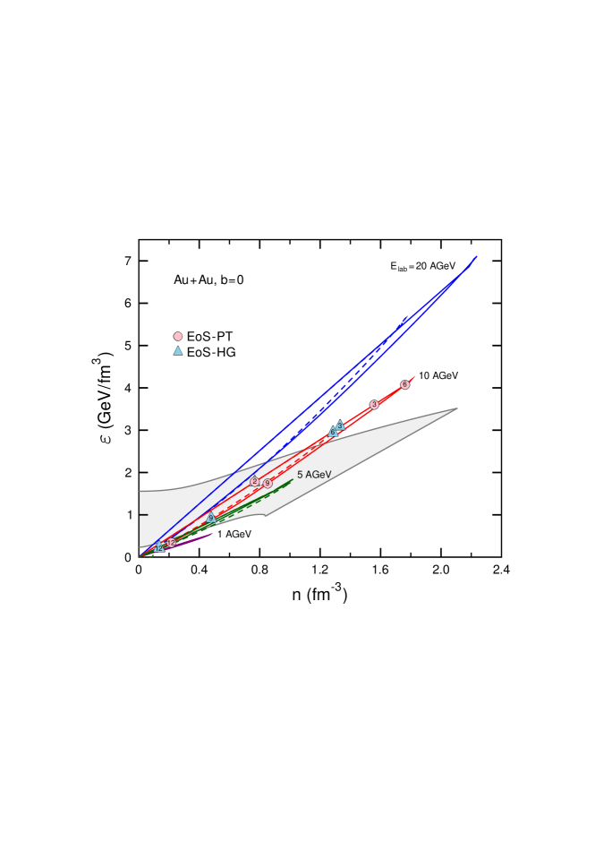
Figure 1: Time evolution of matter in central Au+Au collision at different bombarding energies $E_{\rm\hskip 1.0ptlab}$. Shown are values of energy and baryon densities averaged over the central box. Dashed and solid lines correspond to EoS–HG and EoS–PT, respectively. Numbers in circles and triangles give the c.m. time in fm/$c$. Shading shows the MP region of deconfinement phase transition.

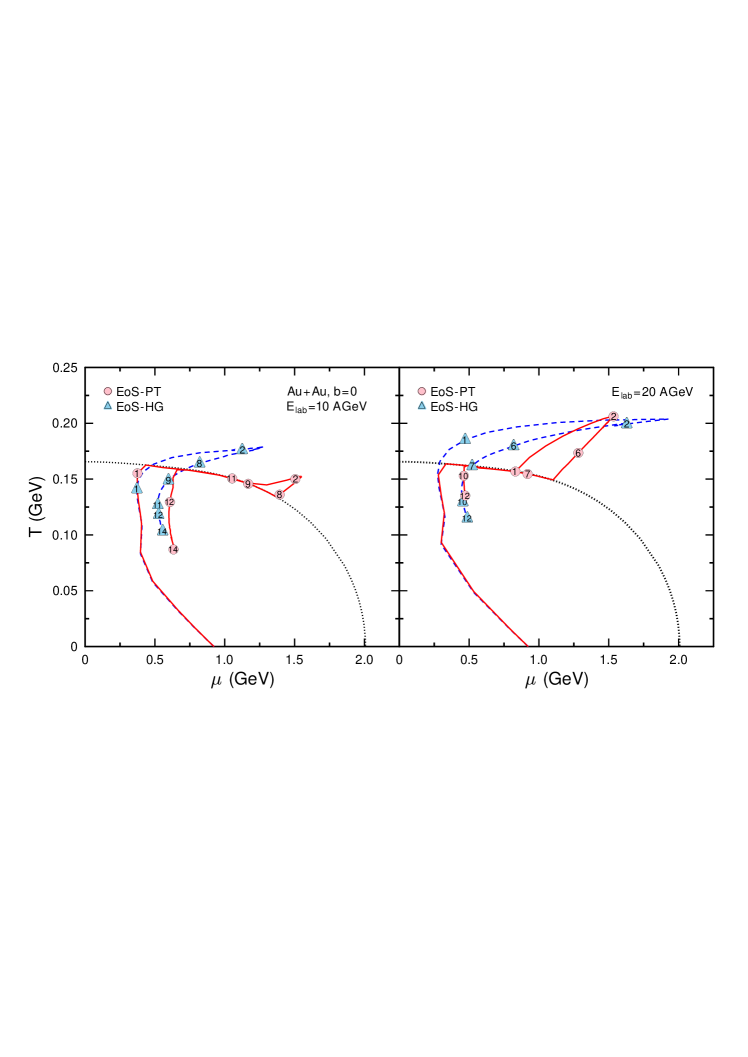
Figure 2: Time evolution of matter (central cell) in the $\mu-T$ plane. Left and right panels correspond to central Au+Au collisions at $E_{\rm\hskip 1.0ptlab}=10$ and 20 AGeV, respectively. Dashed (solid) lines show the results for EoS–HG (EoS–PT). Dotted lines show the MP region. Numbers in circles and triangles give time values in fm/$c$.

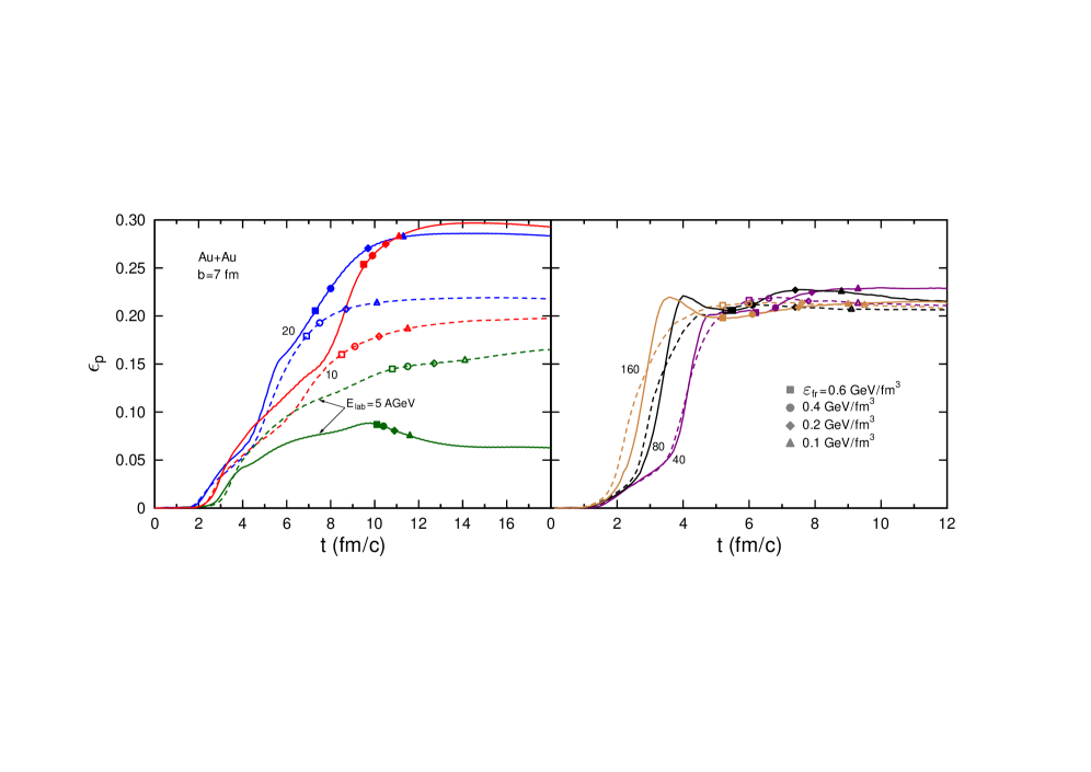
Figure 3: Time dependence of the momentum anisotropy in Au+Au collisions for different bombarding energies ($b=7$ fm). The solid (dashed) lines correspond to the EoS–PT (EoS–HG). Markers show time moments when energy density in the central box becomes lower than certain values $\varepsilon_{\rm{fr}}$ indicated in the the right panel.

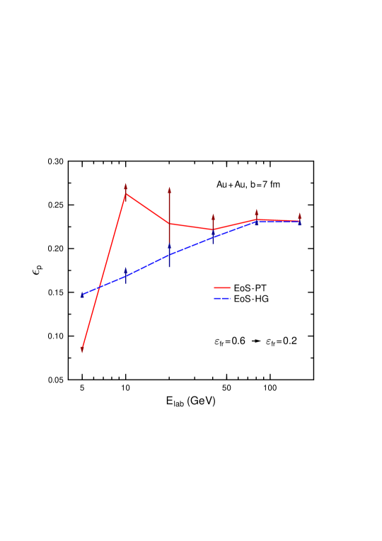
Figure 4: Excitation function of momentum anisotropy in Au+Au collisions with $b=7$ fm. The solid (dashed) lines correspond to the EoS–PT (EoS–HG). Arrows show possible shifts of $\epsilon_{p}$-values for different choices of freeze-out energy density $\varepsilon_{\rm fr}$ between 0.2 and 0.6 GeV/fm³.

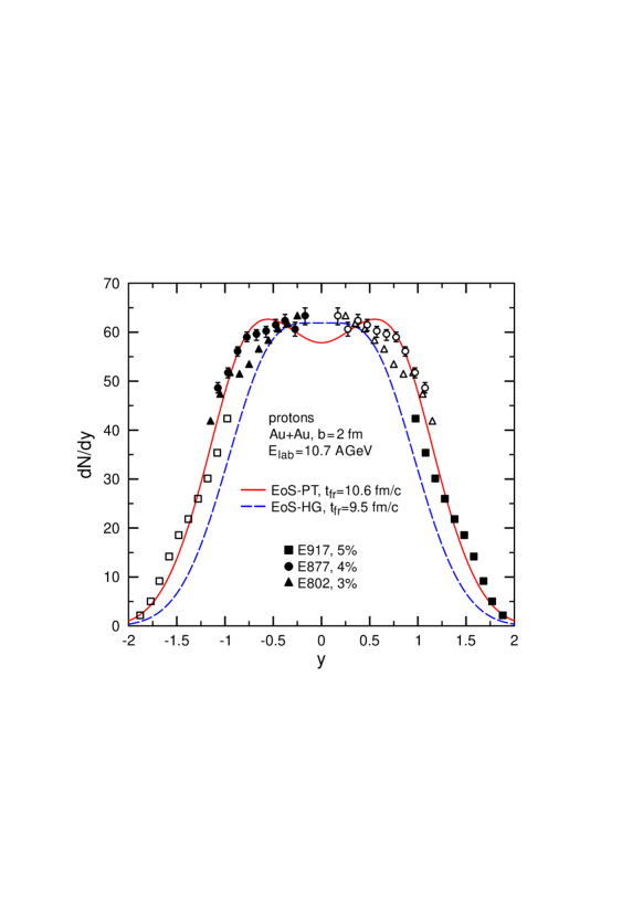
Figure 5: Proton rapidity distributions for central Au+Au collision at $E_{\rm\hskip 1.0ptlab}=10.7$ AGeV. Full symbols are experimental data Ahl98 ; Bac01 ; Bar00 . Open symbols are obtained by reflection with respect to midrapidity.

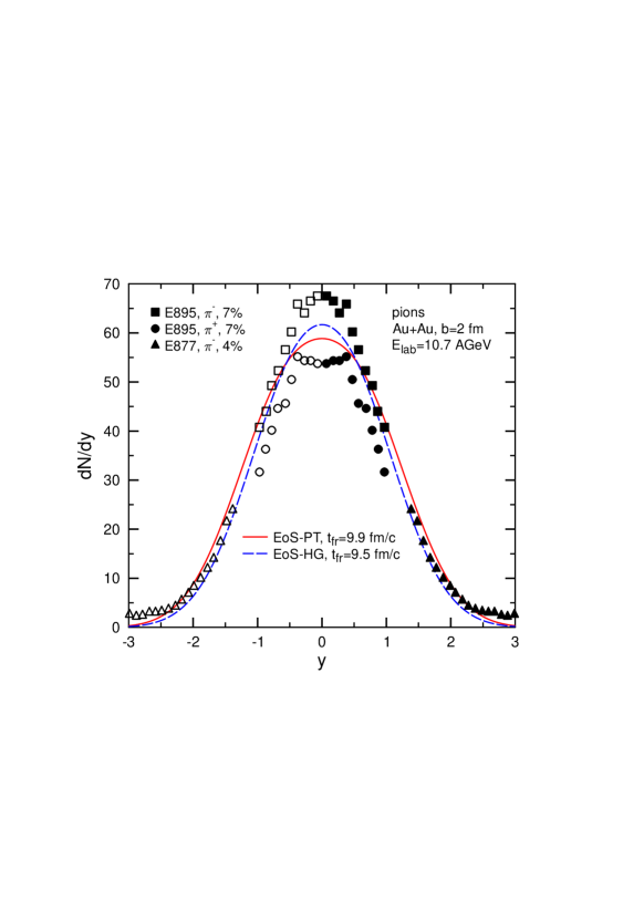
Figure 6: Same as Fig. 5 but for rapidity distributions of $\pi^{-}$ mesons. Experimental data are taken from Refs. Bar00 ; Kla03 .