DESY 10-228 ISSN 0418-9833
December 2010
Measurement of the Inclusive Scattering Cross Section at High Inelasticity and of the Structure Function
H1 Collaboration
A measurement is presented of the inclusive neutral current scattering cross section using data collected by the H1 experiment at HERA during the years 2003 to 2007 with proton beam energies of , , and GeV. The kinematic range of the measurement covers low absolute four-momentum transfers squared, GeV GeV2, small values of Bjorken , , and extends to high inelasticity up to . The structure function is measured by combining the new results with previously published H1 data at GeV and GeV. The new measurements are used to test several phenomenological and QCD models applicable in this low and low kinematic domain.
Submitted to EPJC
F.D. Aaron5,49, C. Alexa5, V. Andreev25, S. Backovic30, A. Baghdasaryan38, S. Baghdasaryan38, E. Barrelet29, W. Bartel11, O. Behrend8,54 P. Belov11, K. Begzsuren35, A. Belousov25, J.C. Bizot27, V. Boudry28, I. Bozovic-Jelisavcic2, J. Bracinik3, G. Brandt11, M. Brinkmann11, V. Brisson27, D. Britzger11, D. Bruncko16, A. Bunyatyan13,38, G. Buschhorn26,†, A. Bylinkin24, L. Bystritskaya24, A.J. Campbell11, K.B. Cantun Avila22, F. Ceccopieri4, K. Cerny32, V. Cerny16,47, V. Chekelian26, A. Cholewa11, J.G. Contreras22, J.A. Coughlan6, J. Cvach31, J.B. Dainton18, K. Daum37,43, B. Delcourt27, J. Delvax4, E.A. De Wolf4, C. Diaconu21, M. Dobre12,51,52, V. Dodonov13, A. Dossanov26, A. Dubak30,46, G. Eckerlin11, S. Egli36, A. Eliseev25, E. Elsen11, L. Favart4, A. Fedotov24, R. Felst11, J. Feltesse10,48, J. Ferencei16, D.-J. Fischer11, M. Fleischer11, A. Fomenko25, E. Gabathuler18, J. Gayler11, S. Ghazaryan11, A. Glazov11, L. Goerlich7, N. Gogitidze25, M. Gouzevitch11,45, C. Grab40, A. Grebenyuk11, T. Greenshaw18, B.R. Grell11, G. Grindhammer26, S. Habib11, D. Haidt11, C. Helebrant11, R.C.W. Henderson17, E. Hennekemper15, H. Henschel39, M. Herbst15, G. Herrera23, M. Hildebrandt36, K.H. Hiller39, D. Hoffmann21, R. Horisberger36, T. Hreus4,44, F. Huber14, M. Jacquet27, X. Janssen4, L. Jönsson20, A.W. Jung15, H. Jung11,4, M. Kapichine9, J. Katzy11, I.R. Kenyon3, C. Kiesling26, M. Klein18, C. Kleinwort11, T. Kluge18, A. Knutsson11, R. Kogler26, P. Kostka39, M. Kraemer11, J. Kretzschmar18, K. Krüger15, K. Kutak11, M.P.J. Landon19, W. Lange39, G. Laštovička-Medin30, P. Laycock18, A. Lebedev25, V. Lendermann15, S. Levonian11, K. Lipka11,51, B. List12, J. List11, N. Loktionova25, R. Lopez-Fernandez23, V. Lubimov24, A. Makankine9, E. Malinovski25, P. Marage4, H.-U. Martyn1, S.J. Maxfield18, A. Mehta18, A.B. Meyer11, H. Meyer37, J. Meyer11, S. Mikocki7, I. Milcewicz-Mika7, F. Moreau28, A. Morozov9, J.V. Morris6, M.U. Mozer4, M. Mudrinic2, K. Müller41, Th. Naumann39, P.R. Newman3, C. Niebuhr11, A. Nikiforov11,53, D. Nikitin9, G. Nowak7, K. Nowak11, J.E. Olsson11, S. Osman20, D. Ozerov24, P. Pahl11, V. Palichik9, I. Panagouliasl,11,42, M. Pandurovic2, Th. Papadopouloul,11,42, C. Pascaud27, G.D. Patel18, E. Perez10,45, A. Petrukhin11, I. Picuric30, S. Piec11, H. Pirumov14, D. Pitzl11, R. Plačakytė12, B. Pokorny32, R. Polifka32, B. Povh13, V. Radescu14, N. Raicevic30, T. Ravdandorj35, P. Reimer31, E. Rizvi19, P. Robmann41, R. Roosen4, A. Rostovtsev24, M. Rotaru5, J.E. Ruiz Tabasco22, S. Rusakov25, D. Šálek32, D.P.C. Sankey6, M. Sauter14, E. Sauvan21, S. Schmitt11, L. Schoeffel10, A. Schöning14, H.-C. Schultz-Coulon15, F. Sefkow11, L.N. Shtarkov25, S. Shushkevich26, T. Sloan17, I. Smiljanic2, Y. Soloviev25, P. Sopicki7, D. South11, V. Spaskov9, A. Specka28, Z. Staykova11, M. Steder11, B. Stella33, G. Stoicea5, U. Straumann41, T. Sykora4,32, P.D. Thompson3, T. Toll11, T.H. Tran27, D. Traynor19, P. Truöl41, I. Tsakov34, B. Tseepeldorj35,50, I. Tsurin18, J. Turnau7, K. Urban15, A. Valkárová32, C. Vallée21, P. Van Mechelen4, A. Vargas11, Y. Vazdik25, M. von den Driesch11, D. Wegener8, E. Wünsch11, J. Žáček32, J. Zálešák31, Z. Zhang27, A. Zhokin24, H. Zohrabyan38, and F. Zomer27
1 I. Physikalisches Institut der RWTH, Aachen, Germany
2 Vinca Institute of Nuclear Sciences, University of Belgrade,
1100 Belgrade, Serbia
3 School of Physics and Astronomy, University of Birmingham,
Birmingham, UKb
4 Inter-University Institute for High Energies ULB-VUB, Brussels and
Universiteit Antwerpen, Antwerpen, Belgiumc
5 National Institute for Physics and Nuclear Engineering (NIPNE) ,
Bucharest, Romaniam
6 Rutherford Appleton Laboratory, Chilton, Didcot, UKb
7 Institute for Nuclear Physics, Cracow, Polandd
8 Institut für Physik, TU Dortmund, Dortmund, Germanya
9 Joint Institute for Nuclear Research, Dubna, Russia
10 CEA, DSM/Irfu, CE-Saclay, Gif-sur-Yvette, France
11 DESY, Hamburg, Germany
12 Institut für Experimentalphysik, Universität Hamburg,
Hamburg, Germanya
13 Max-Planck-Institut für Kernphysik, Heidelberg, Germany
14 Physikalisches Institut, Universität Heidelberg,
Heidelberg, Germanya
15 Kirchhoff-Institut für Physik, Universität Heidelberg,
Heidelberg, Germanya
16 Institute of Experimental Physics, Slovak Academy of
Sciences, Košice, Slovak Republicf
17 Department of Physics, University of Lancaster,
Lancaster, UKb
18 Department of Physics, University of Liverpool,
Liverpool, UKb
19 Queen Mary and Westfield College, London, UKb
20 Physics Department, University of Lund,
Lund, Swedeng
21 CPPM, Aix-Marseille Université, CNRS/IN2P3, Marseille, France
22 Departamento de Fisica Aplicada,
CINVESTAV, Mérida, Yucatán, Méxicoj
23 Departamento de Fisica, CINVESTAV IPN, México City, Méxicoj
24 Institute for Theoretical and Experimental Physics,
Moscow, Russiak
25 Lebedev Physical Institute, Moscow, Russiae
26 Max-Planck-Institut für Physik, München, Germany
27 LAL, Université Paris-Sud, CNRS/IN2P3, Orsay, France
28 LLR, Ecole Polytechnique, CNRS/IN2P3, Palaiseau, France
29 LPNHE, Université Pierre et Marie Curie Paris 6,
Université Denis Diderot Paris 7, CNRS/IN2P3, Paris, France
30 Faculty of Science, University of Montenegro,
Podgorica, Montenegroe
31 Institute of Physics, Academy of Sciences of the Czech Republic,
Praha, Czech Republich
32 Faculty of Mathematics and Physics, Charles University,
Praha, Czech Republich
33 Dipartimento di Fisica Università di Roma Tre
and INFN Roma 3, Roma, Italy
34 Institute for Nuclear Research and Nuclear Energy,
Sofia, Bulgariae
35 Institute of Physics and Technology of the Mongolian
Academy of Sciences, Ulaanbaatar, Mongolia
36 Paul Scherrer Institut,
Villigen, Switzerland
37 Fachbereich C, Universität Wuppertal,
Wuppertal, Germany
38 Yerevan Physics Institute, Yerevan, Armenia
39 DESY, Zeuthen, Germany
40 Institut für Teilchenphysik, ETH, Zürich, Switzerlandi
41 Physik-Institut der Universität Zürich, Zürich, Switzerlandi
42 Also at Physics Department, National Technical University,
Zografou Campus, GR-15773 Athens, Greece
43 Also at Rechenzentrum, Universität Wuppertal,
Wuppertal, Germany
44 Also at University of P.J. Šafárik,
Košice, Slovak Republic
45 Also at CERN, Geneva, Switzerland
46 Also at Max-Planck-Institut für Physik, München, Germany
47 Also at Comenius University, Bratislava, Slovak Republic
48 Also at DESY and University Hamburg,
Helmholtz Humboldt Research Award
49 Also at Faculty of Physics, University of Bucharest,
Bucharest, Romania
50 Also at Ulaanbaatar University, Ulaanbaatar, Mongolia
51 Supported by the Initiative and Networking Fund of the
Helmholtz Association (HGF) under the contract VH-NG-401.
52 Absent on leave from NIPNE-HH, Bucharest, Romania
53 Now at Humbold Universität Berlin, Berlin, Germany
54 Now at Siemens, Nürnberg, Germany
† Deceased
a Supported by the Bundesministerium für Bildung und Forschung, FRG,
under contract numbers 05H09GUF, 05H09VHC, 05H09VHF, 05H16PEA
b Supported by the UK Science and Technology Facilities Council,
and formerly by the UK Particle Physics and
Astronomy Research Council
c Supported by FNRS-FWO-Vlaanderen, IISN-IIKW and IWT
and by Interuniversity
Attraction Poles Programme,
Belgian Science Policy
d Partially Supported by Polish Ministry of Science and Higher
Education, grant DPN/N168/DESY/2009
e Supported by the Deutsche Forschungsgemeinschaft
f Supported by VEGA SR grant no. 2/7062/ 27
g Supported by the Swedish Natural Science Research Council
h Supported by the Ministry of Education of the Czech Republic
under the projects LC527, INGO-LA09042 and
MSM0021620859
i Supported by the Swiss National Science Foundation
j Supported by CONACYT,
México, grant 48778-F
k Russian Foundation for Basic Research (RFBR), grant no 1329.2008.2
l This project is co-funded by the European Social Fund (75%) and
National Resources (25%) - (EPEAEK II) - PYTHAGORAS II
m Supported by the Romanian National Authority for Scientific Research
under the contract PN 09370101
1 Introduction
Deep inelastic lepton-nucleon scattering (DIS) plays a pivotal role in determining the structure of the proton. The electron-proton collider HERA covers a wide range of absolute four-momentum transfer squared, , and of Bjorken . Previous measurements of the DIS cross section, performed by the H1 [1, 2, 3, 4, 5, 6] and ZEUS [7, 8, 9, 10, 11, 12, 13, 14, 15] collaborations, using data at proton beam energies of GeV and GeV and a lepton beam energy of GeV, as well as their combination [16], have enabled studies of perturbative Quantum Chromodynamics (QCD) with unprecedented precision. These measurements are complemented here with new data including the data taken at GeV and GeV.
At low , the scattering cross section is defined by the two structure functions, and . In a reduced form, the double differential cross section is given by
| (1) |
Here is the fine structure constant and is the process inelasticity which is related to and the centre-of-mass energy squared by . The two structure functions are defined by the cross sections for the scattering of the longitudinally and transversely polarised photons off protons and as
| (2) | |||||
| (3) |
These relations are valid to good approximation at low and imply that . To disentangle the two structure functions in a model-independent way, measurements at different values of are required.
Using the ratio , defined as
| (4) |
the reduced cross section in equation 1 can also be written as
| (5) |
where .
In the quark-parton model, is given by the charge squared weighted sum of the quark densities while is zero because of helicity conservation. In QCD, the gluon emission gives rise to a non-vanishing . Measuring the structure function therefore provides a way of studying the gluon density and a test of perturbative QCD.
The contribution of the term containing to the scattering cross section can be sizeable only at large values of . For low values of , the reduced DIS neutral current (NC) scattering cross section is well approximated by the structure function . Kinematically, for low , large values of correspond to low energies of the scattered lepton. Selecting high events is thus complicated due to a possibly large background from hadronic final state particles.
This paper reports new measurements of the DIS cross section at low and high values, using data collected by the H1 collaboration in the years to . The data samples are taken with dedicated high and low triggers. Methods relying on data are used to determine the hadronic background contribution. The first data sample consists of a new cross-section measurement for the nominal proton beam energy of GeV for GeV2 with an increased integrated luminosity of pb-1 compared to [2]. The second new data sample at GeV covers the region GeV2 using a dedicated silicon tracker for the measurement of the charge of backward scattered particles. This analysis is based on an integrated luminosity of pb-1. Two further data samples correspond to the measurements at reduced proton beam energy, GeV and GeV, covering the kinematic domain of GeV2 with integrated luminosities of pb-1 and pb-1, respectively. Combined with the previously published H1 measurements [1, 2], the data are used to measure the structure function . This new measurement supersedes the previous H1 result [17].
The measurements are used to test several phenomenological and QCD models describing the low behaviour of the DIS cross section. The phenomenological models include the power-law dependence of [18] and several dipole models [19, 20, 21, 22, 23] applicable at low . For the first time, dipole model analyses are extended to account for the non-negligible valence-quark contributions at small . Fits using the DGLAP evolution equations [24, 25, 26, 27, 28] at NLO [29, 30] are applied for GeV2. For the DGLAP fits, different treatments of the heavy quark contributions are compared [31, 32, 33]. A study of possible non-DGLAP contributions at low and low is performed by varying kinematic cuts applied to the data. The dipole and DGLAP models are compared to with other by performing fits in a common kinematic domain.
This paper is organised as follows. The measurement technique is presented in section 2. The data analysis and event selection are described in section 3. The cross section and measurement procedures are explained in sections 4 and 5. Section 6 contains the phenomenological analysis of the measurement. The results presented in the paper are summarised in section 7.
2 Measurement Technique
2.1 H1 Detector
A detailed description of the H1 detector can be found in [34, 35]. A view of a high , low event reconstructed in the H1 detector is shown in figure 1. The origin of the H1 coordinate system is the nominal interaction point. The direction of the proton beam defines the positive -axis (forward direction). Transverse momenta are measured in the plane. Polar () and azimuthal () angles are measured with respect to the reference system.
The most relevant detector components for this analysis are the central tracker (CT), the backward lead-scintillator calorimeter (SpaCal) [36] and the liquid argon calorimeter (LAr) [37]. The central tracker consists of the central jet drift chambers (CJC1 and CJC2), the drift chamber [38], the central inner proportional chamber (CIP) [39], the central silicon tracker (CST) [40]. The detector operates in a T solenoidal magnetic field. The drift chambers and the CST are used for the measurement of tracks from the hadronic final state and to determine the interaction vertex. The energy of the scattered lepton is measured by the SpaCal. The polar angle of the scattered lepton is determined by the SpaCal and the vertex position. The tracking information obtained from the backward silicon tracker (BST) [41], partially in combination with the CJC, determines the charge of the scattered electron candidate using the measured curvature. The BST is equipped with silicon pad sensors to provide a fast trigger signal. The SpaCal contains electromagnetic and hadronic sections. Its energy resolution for electromagnetic energy depositions is . It also provides a trigger based on the scattered lepton energy, time and location inside the calorimeter. The LAr allows the hadronic final state to be reconstructed. Its energy resolution was determined to be with pion test beam data [42]. Two electromagnetic calorimeters, a tungsten/quartz-fibre sampling calorimeter (“photon tagger”) and a compact lead/scintillator calorimeter (“electron tagger”), are located close to the beam pipe at m and m, respectively. The photon tagger is used for monitoring the luminosity via the measurement of the Bethe-Heitler process . The electron tagger is used to select pure samples of photoproduction events used for background estimation.
The H1 data collection employs a four level trigger system. The first level trigger (L1) is based on various sub-detector components, which are combined at the second level (L2); the decision is refined at the third level (L3). The fully reconstructed events are subject to an additional selection at the software filter farm (L4).
2.2 Reconstruction
At HERA, the DIS kinematics can be reconstructed using the scattered lepton, the hadronic final state or a combination of both. For the measurement at high inelasticity , however, the reconstruction of kinematics using the scattered lepton, the so called electron method, has superior resolution and is used here.
The kinematic variables in the electron method are determined by
| (6) |
Energy-momentum conservation implies that
| (7) |
where the subscripts “in” and “out” denote the total before and after the interaction, () is the reconstructed energy (longitudinal component of the momentum) of a particle from the hadronic final state and the sum runs over all measured hadronic final state particles. For events with hard QED initial state radiation (ISR), the radiated photon escapes in the beam pipe and is reduced. Therefore measurement of allows control of the effective beam energy and the reduction of contamination from ISR events. Requiring to be close to the nominal value also suppresses photoproduction background events, in which the scattered lepton escapes in the beam pipe.
2.3 Monte Carlo Simulation
The Monte Carlo (MC) simulation is used to correct for detector acceptance and resolution effects. The inclusive DIS signal events are generated using the DJANGOH [43] event generator, which also contains a simplified simulation of difractive processes. Elastic QED Compton events are generated using the COMPTON event generator [44]. The cross section measurement is corrected for QED radiation up to order using HERACLES [45] which is included in DJANGOH. The radiative corrections are cross checked with HECTOR [46].
All generated events are passed through the full GEANT [47] based simulation of the H1 apparatus and are reconstructed using the same program chain as the data. Shower models are used to speed up the simulation in the LAr [48] and SpaCal [49] calorimeters. The calibrations of the SpaCal and the LAr, as well as the alignment, are performed for the reconstructed MC events in the same way as for the data.
3 Data Analysis
3.1 Data Sets and Event Selection
The analysis is based on several data samples which are listed in table 1. These samples are distinguished based on the kinematic region, online trigger condition, offline selection criteria and proton beam energy.
3.1.1 Online Event Selection
| Sample | Years | range | Total | ||
|---|---|---|---|---|---|
| GeV2 | pb-1 | pb-1 | pb-1 | ||
| Medium CJC GeV | - | ||||
| Low BST GeV | - | ||||
| GeV | — | ||||
| GeV | — |
The two high data samples for GeV (‘medium CJC GeV’ and ’low BST GeV’) are collected with dedicated low energy SpaCal triggers which require at L1 a compact energy deposit in the SpaCal with energy above GeV. In addition, to suppress non- background, a CIP track segment pointing to the nominal interaction vertex position is required. Several additional veto conditions, which are based on scintillator counters positioned up- and downstream the nominal interaction region and on the hadronic section of the SpaCal are used to further suppress non- background.
The medium CJC GeV analysis uses an L2 trigger condition, which requires that the energy deposit is reconstructed in the outer SpaCal region, at distances from the beam line of cm, corresponding approximately to the inner CJC acceptance. The low BST GeV analysis uses another L2 condition, which requires cm corresponding to the acceptance of the BST. Both triggers are further filtered at L4 using fully reconstructed events to validate low level trigger conditions.
For the reduced proton beam energy data, the main trigger is the SpaCal trigger with an energy threshold of GeV. In addition a track segment has to be reconstructed in the BST pad detector or the CIP. This trigger is complemented with a SpaCal trigger at a higher energy threshold of GeV and no tracking condition. No L4 filtering is imposed for the low runs.
The data are subject to offline cuts which are listed in table 2 and discussed below. Some of the cuts are common to all data samples, others differ, primarily because of the different tracking conditions used for the scattered lepton validation.
In order to ensure an accurate kinematic reconstruction and to suppress non- background, the coordinate of the interaction vertex, , is required to be reconstructed close to the nominal position and with sufficient accuracy, .
The scattered lepton is identified with the localised energy deposition (cluster) reconstructed in the SpaCal calorimeter, which has the highest transverse energy . Here is calculated using the cluster energy and position, the event interaction vertex position and the beam line. If the highest cluster does not satisfy all of the identification cuts mentioned below, the cluster with the second highest is tried. The procedure is repeated for up to three clusters. If none of the three clusters satisfies the selection cuts, the event is rejected.
3.1.2 Offline Event Selection
| Selection criteria | Medium CJC | Low BST | GeV |
|---|---|---|---|
| GeV | GeV | and GeV | |
| Vertex position | cm | ||
| Vertex precision | cm | ||
| Scattered lepton energy | GeV | ||
| Radial cluster position | cm | cm | cm |
| Cluster transverse shape | |||
| cm for cm | |||
| cm | cm | — | |
| Energy in hadronic section | |||
| Tracker validation | cm | cm | |
| Lepton charge | Agree with beam charge for | ||
| Energy-momentum match | — | for GeV | |
| Longitudinal momentum balance | GeV | ||
| Total energy in hadronic SpaCal | — | — | GeV |
| QED Compton rejection | Topological veto | ||
| Kinematic range | GeV2 | GeV2 | GeV2 |
The energy of the scattered lepton is required to exceed GeV to ensure a high trigger efficiency. The radial position of the scattered lepton is required to be well inside the SpaCal acceptance and within the active trigger region.
Several cuts are applied to suppress photoproduction background. In photoproduction events, hadronic final state particles may scatter in the SpaCal calorimeter and mimic the electron signal. The main sources of such background are charged hadrons (pions, kaons and (anti-)protons) as well as decays for which one of the photons converts into an pair prior to entering the tracking devices. The selection against photoproduction events includes cuts on the transverse shower radius, estimated using logarithmic () and square root (ECRA) energy weighting [49], as well as the fraction of energy of the cluster contained in the four highest energy cells, . The cut is found to be more efficient than the cluster radius estimators, but an L4 condition requires the ECRA cut to be used for the GeV analyses. The transverse shape requirements are efficient against hadronic background as well as background from where the two photon clusters merge together.
The cut on the fraction of energy in the hadronic SpaCal behind the lepton candidate cluster, , rejects purely hadronic background. The cut does not reject background for cm because of the limited acceptance of the hadronic SpaCal. As a compromise between signal efficiency and background rejection, an extra cut cm is introduced for cm.
The photoproduction background is suppressed further by requiring cluster validation by a track (“track link”). The medium CJC GeV analysis uses tracks reconstructed solely in the CJC tracker. The other analyses use a dedicated reconstruction algorithm which combines information obtained from the CJC, BST, event vertex and the SpaCal (“BC” algorithm [50]). The tracks are extrapolated to the SpaCal position and required to match the SpaCal cluster within cm for the CJC reconstruction and within cm for the BC algorithm. The tighter cut on the track-cluster matching for the BC compared to the CJC algorithm is possible for low because of accurate BST reconstruction and for higher because the SpaCal cluster is used in the BC algorithm and pulls the track towards the cluster. As discussed below, in section 3.2, the measured scattered lepton charge is required to match the beam charge for . The sample for which the charges are different is used to estimate the remaining background. For GeV, the momentum reconstruction is accurate enough and is required, where is the track momentum of the electron candidate.
The total energy reconstructed in the hadronic section of the SpaCal, , is required to be below GeV for the GeV and GeV data. This avoids a trigger inefficiency arising from a veto on the total energy deposited in the hadronic SpaCal.
Events with high energy initial state photon radiation are rejected by requiring GeV. This cut is also efficient against the photoproduction background. The QED Compton process, , is suppressed using a topological cut against events with two back-to-back electromagnetic clusters reconstructed in the SpaCal.
Distributions of the variables which are used for the scattered lepton identification are shown for the GeV sample in figure 2. While the shapes observed in the data are sometimes not perfectly reproduced by the simulation, those differences occur far from the cut values. The electron identification selection criteria are designed to have high efficiency for the signal while rejecting a significant amount of the background.
3.2 Background Subtraction
At low , corresponding to high , the background contribution after the event selection is of a size comparable to the DIS signal. To reduce the systematic uncertainty, the background determination in this analysis relies on data. Two distinct methods are applied depending on the event inelasticity . For high , the background estimation is based on a sample of events, in which the charge of the lepton candidate is opposite to the beam charge (“wrong charge method”). For lower the background contamination is small, however, the uncertainty due to the charge determination becomes large, and an alternative method is employed. In this method the background is estimated using a sub-sample of events, in which the scattered lepton is detected in the electron tagger (“tagger method”).
The wrong charge subtraction method relies on the approximate charge symmetry of the background and a good charge reconstruction with the tracker at low momenta. The residual charge asymmetry of the background is defined as
| (8) |
where is the number of background events in which the lepton candidate is associated with a positively (for ) and a negatively (for ) charged track. The charge asymmetry of the background arises from the different response of the SpaCal to particles compared to antiparticles (in particular and ) and detector misalignments. The asymmetry depends on the electron identification cuts since they alter the ratio of the electromagnetic to hadronic components of the background.
The charge asymmetry is measured directly from the data by comparing background estimates from the and scattering periods as well as using clean background samples with the scattered lepton measured in the electron tagger. The charge asymmetry of the background is found to deviate from unity by and for scattering angles between and .
The scattered lepton charge may be misidentified which leads to an overestimation of the background at . The charge reconstruction is studied in the background free sample at GeV by comparing events with correctly and wrongly reconstructed lepton charge. The fraction of wrongly reconstructed events depends on both the energy and the angle of the scattered electron. This dependence is well reproduced by the simulation. The fraction is smaller at small due to a larger track curvature and at small since the CJC has a better momentum resolution than the BST.
Charge reconstruction at low energy ( GeV) is studied using events with initial state radiation in which the radiative photon is detected in the photon tagger. For these events, the sum of the scattered electron and photon energies, , peaks at the beam energy which allows the estimation of the residual background using a side-band method. This procedure is illustrated for the combined GeV and GeV dataset in figure 3. The DIS signal is approximated by a Gaussian while the background is assumed to follow an exponential distribution. The Gaussian width of the signal distribution is fixed to be the same for both lepton candidate charges. The data are fitted by the sum of signal and background hypotheses. From these fits, the fraction of events with wrongly reconstructed charge in the data is determined to be , compared to in the simulation. The simulation is corrected for the difference and a systematic uncertainty of is used for the charge determination of the lepton candidate.
The tagger method of background estimation used at low relies on an accurate determination of the tagger acceptance, , which is defined in this analysis as the fraction of background events in which the scattered electron is tagged. The acceptance is measured by comparing all wrong charge events with GeV passing nominal selection cuts to those in which a scattered electron candidate is detected in the electron tagger. For this selection, the wrong charge sample is almost entirely comprised of photoproduction events with a small admixture of DIS events with charge misidentification, which is subtracted using the MC estimate. The tagger acceptance is seen to vary between for the medium CJC GeV sample, taken in the year , and for the GeV sample. This difference in acceptance may be explained by differences in the beam optics. Stability of the tagger acceptance for different kinematic ranges is studied by varying the and cuts. A systematic uncertainty of is assigned to the tagger acceptance. This uncertainty also accounts for a potential variation of the acceptance as a function of and . Finally, to avoid a subtraction of overlapping DIS and Bethe-Heitler events containing energy deposits in the electron tagger, in the background estimation the tagged events are also required to have a charge opposite to the lepton beam charge. Neglecting the background charge asymmetry, this reduces the number of tagged background events by a factor of two.
To summarise, the number of signal events for the and running periods is estimated as
| (9) |
Here () is the number of events with the charge of the lepton candidate the same as (opposite to) the lepton beam charge and is the number of tagged events with the charge of the lepton candidate opposite to the lepton beam charge.
3.3 Efficiencies
The efficiency of the electron identification cuts is studied in the data and MC, and the simulation is adjusted accordingly.
3.3.1 Online Selection and Vertex Efficiency
The efficiencies of the triggers used in the analysis are determined using events collected with independent triggers. The efficiency of the L1 energy condition is checked with tracker-based triggers. It is found to be fully efficient for GeV.
The efficiency of the L1 tracking condition (CIP or BST for GeV and GeV data) is checked using events triggered by SpaCal-based triggers without tracking conditions. The efficiency of the L1 tracking condition is correlated with the vertex efficiency. To avoid biases, a combined efficiency is calculated as
| (10) |
where is the CIP or BST L1 condition efficiency based on events without vertex cut and is the vertex efficiency for the events passing the CIP or BST tracking condition. A similar decomposition is used for the condition, used for GeV data.
The CIP L1 condition is found to have uniform efficiency for cm, i.e. within the CIP acceptance. The efficiency varies for different periods between and . For lower radii, the efficiency decreases by about since the scattered lepton leaves the CIP acceptance. This region is covered by the BST pad detector and for the combined condition, there is no drop of the efficiency.
The efficiency decreases at low cm and high since the scattered lepton as well as part of the hadronic final state leave the CJC acceptance. The decrease in the efficiency occurs mostly for diffractive events which have a rapidity gap between the proton remnant and the struck quark. For cm at , the inefficiency in the data reaches compared to in the Monte Carlo simulation. The difference in the efficiency is parameterised as a function of and and is applied to the simulation.
3.3.2 Offline Selection Efficiency
The determination of the offline electron selection efficiencies at high is complicated due to the large background contamination. Thus an accurate estimation of the background is a matter of paramount importance for this analysis. As discussed in section 3.2, this estimation is provided by the wrong charge data sample, for which a track link is required for the lepton candidate.
The track-link efficiency is measured using a background free sample with GeV and no track condition, as the fraction of events satisfying the track link requirement.
For the medium CJC GeV sample, the SpaCal cluster is linked with a track from the CJC. It is observed that the track-link efficiency has a radial dependence which is well reproduced by the MC simulation. For the overall level of inefficiency, however, the MC prediction has to be downgraded by , and for the -, - and the - running periods, respectively. The track-link efficiency for the low BST GeV, GeV and GeV analyses has radial and azimuthal dependencies in the BST and BST-CJC overlap regions. It has a typical value of but drops in some regions to . The simulation is corrected in radial steps of cm in the cm range for the BST azimuthal sectors individually. This correction does not exceed . The correction factors to the MC are applied for all lepton energies. A cross check for low events is performed using a sample of ISR events for which a good agreement between the data and corrected MC is observed.
The transverse and longitudinal distributions of the electromagnetic shower energies (“shower shapes”) are affected by the amount of material passed through by the scattered lepton before entering the calorimeter. The total amount of material before the SpaCal depends on the scattering angle and varies between and radiation lengths. A detailed map of the detector material is included in the simulation. The distribution of the material in the CT is checked using reconstructed photon conversions and nuclear interactions. A significant contribution to the material budget is due to the BST sensors, cooling circuit and readout electronics. The contribution due to the readout electronics is determined using the transverse shower shapes. The method exploits the fact that the BST was removed from the H1 detector for repair during the data taking. A comparison of the shower shapes in the data and MC simulation for the 2005 and 2006 data taking periods thus allows a check of the BST material contribution with high accuracy.
The signal efficiencies of the other offline selection cuts listed in table 2 are studied after the background subtraction described in section 3.2. Since the background is large and its level typically varies significantly upon applying these cuts, a variation of the background asymmetry is also considered for each cut of the electron identification. The background subtraction is the dominant systematic uncertainty for the efficiency determination. It is measured with accuracy for , with for and with for .
3.4 Calibration and Alignment
The alignment and calibration of the H1 detector follows a procedure similar to that described in [1]. The alignment starts with the internal alignment of the CT and proceeds to the backward detectors, SpaCal and BST. The alignment of the BST sensors is performed with the minimisation package Millepede [51] by using position information from the central tracker and the SpaCal. The global alignment of the BST is refined by requiring a matching between the momentum and energy measurements in the BST, CJC and the SpaCal [50].
The calibration of the SpaCal electromagnetic energy scale uses the double angle method [1]. The linearity of the SpaCal energy response is checked using , and QED Compton events.
The hadronic final state is reconstructed using information from the central tracker, the LAr calorimeter and the SpaCal. The tracker momentum scale is checked by reconstructing narrow resonances such as and decays. The hadronic calibration of the LAr calorimeter employs the transverse energy balance between the scattered electron and the hadronic final state as described in [1]. The hadronic calibration of the SpaCal employs the longitudinal momentum balance. The relative contribution of the SpaCal to becomes large at high and the absolute calibration is obtained for GeV by requiring to peak at for both the data and the Monte Carlo simulation. The calibration constants are determined separately for the electromagnetic and hadronic sections of the SpaCal.
3.5 Radiative Corrections
For large inelasticity and low the kinematics reconstruction using the electron method is prone to large radiative corrections which can reach a level of more than of the Born cross section. Studies based on the DJANGO and HECTOR programs show that the largest radiative contribution arises because of hard initial state radiation from the incoming lepton.
The hard ISR process is strongly suppressed by the cut GeV. After this cut, the radiative corrections amount to about of the Born cross section with no strong dependence on . A slight increase in the corrections occurs at the highest due to QED Compton events. These events are efficiently rejected using the topological cut against two back-to-back clusters in the SpaCal.
Events rejected by the cut GeV can be used to study the description by the simulation of the hard ISR. This is illustrated in figure 4 which shows the background subtracted distribution for events passing all cuts excluding the cut for the GeV sample. The sample is restricted to GeV which corresponds to . A prominent peak for GeV corresponds to the hard ISR process. The data in this kinematic region are well described by the simulation.
3.6 Control Distributions
Data and MC distributions of the main quantities used to reconstruct the event kinematics for the events passing all selection criteria are compared in figures 5 to 8 for all data sets included in the analysis. The MC distributions are normalised to the integrated luminosity and corrected for selection efficiency differences, as explained above. The control distributions illustrate the considerable level of background for low , that is estimated from the data. The DIS simulation uses the H1PDF2009 set of parton distributions [2]. There is a good overall agreement observed between the measurements and predictions. The local residual differences, visible for the energy distribution in the lowest , BST sample near to GeV and corresponding to (figure 7a and figure 7d ), do not affect the cross-section measurement.
3.7 Systematic Uncertainties
The systematic uncertainty on the cross-section measurements arises from several contributions. Besides the global normalisation uncertainty, these contributions are classified as correlated uncertainties, which affect measurements at different in a correlated manner, and as uncorrelated ones, for which each of the measurements is affected individually. The summary of all systematic uncertainties is given in table 3.
The global normalisation uncertainty is for the GeV period and for the GeV and GeV analyses. The uncertainty includes the uncertainty of the luminosity measurement as well as global trigger and reconstruction efficiency uncertainties.
The uncertainty on the SpaCal electromagnetic energy scale is determined to be at GeV increasing to at GeV for all but the medium CJC GeV analysis. The latter covers a large period of runs, from the year to , and therefore is prone to variations of the SpaCal performance. For this analysis the scale uncertainty is at increasing to at GeV. The uncertainty at around GeV is estimated from the difference between the result of the double-angle calibration and the position of the kinematic peak. The uncertainty at GeV is obtained using and decays [1].
The uncertainty on the lepton polar angle is mrad, which covers uncertainties of the alignment of the SpaCal as well as of the cluster position determination.
The hadronic energy scale has an uncertainty of . Apart from reconstruction in the LAr calorimeter and in the tracker, this value covers the uncertainty of the hadronic energy scale of the SpaCal, which is important at high . The uncertainty of the LAr electronic noise and beam related background is . These uncertainties have little impact on the cross-section measurement which is based on the electron method since they enter only via the cut.
The background charge asymmetry is determined with a precision of . It affects only the data for where the wrong charge subtraction method is used. Its uncertainty has negligible impact on the medium CJC GeV and low BST GeV measurements since these are based on both and HERA running periods and have a charge symmetric background sample. For the GeV and GeV runs, the impact on the cross section reaches at .
| Correlated uncertainty source | Uncertainty |
|---|---|
| Global normalisation | for GeV run |
| for GeV and GeV run | |
| energy scale | at to at GeV |
| (all, but medium CJC GeV) | |
| at to at GeV | |
| (medium CJC GeV) | |
| Polar angle | mrad |
| Hadronic energy scale | |
| LAr noise | |
| Background charge asymmetry | |
| Electron tagger acceptance | |
| Uncorrelated uncertainty source | Uncertainty |
| Trigger efficiency | |
| Track-cluster link efficiency | |
| Lepton charge determination | |
| Electron identification efficiency | |
| Radiative corrections |
The electron tagger acceptance is known to . This uncertainty is applied for only and, since the background at low is small, this source does not have a significant impact on the measurement.
The uncorrelated systematic uncertainties include the Monte Carlo statistical errors and the following sources: the uncorrelated part of the trigger efficiency, known to ; the track-cluster link efficiency, known to ; the uncertainty of the lepton charge determination of leading to uncertainty of the cross section, for only; the electron identification uncertainty varies from for to for ; the uncertainty due to the radiative corrections is determined to be .
4 Cross Section Determination
4.1 Method
At low the contributions to the NC scattering process are completely dominated by photon exchange with negligible differences between the and scattering cross sections. The background determination at high is based on the measured lepton-candidate charge. In order to reduce the sensitivity to the background charge asymmetry, the cross section is determined for a charge symmetric data sample for the medium CJC GeV and the low BST GeV samples. The reduced cross section is calculated in this case for each bin as
| (11) |
Here () is the integrated luminosity for the data (MC), is the number of signal events in the MC and is the value of the reduced cross section in the MC.
Equation 11 is rather insensitive to the uncertainty of the background charge asymmetry since for , the total background is estimated as . The statistical accuracy of equation 11 is limited by the sample with the smaller luminosity, therefore the data taking strategy was tuned to obtain and samples of about equal size.
For the GeV and GeV samples, the absence of data does not allow for usage of equation 11, and a more standard cross section determination formula is used as
| (12) |
These cross sections are therefore more sensitive to the uncertainty in .
| Sample | Bin boundaries in | |||||||||
|---|---|---|---|---|---|---|---|---|---|---|
| GeV | ||||||||||
| GeV | ||||||||||
| GeV | ||||||||||
The medium CJC GeV and low BST GeV samples extend the published H1 measurements to high and for them the same mixed binning is adapted as used in [1]. The GeV and GeV samples are used to measure the structure function . For this measurement, an optimal binning is in with the boundaries of the bins adjusted so that the corresponding values agree for different . This binning is given in table 4. Bin centres are calculated as an arithmetic average of the bin boundaries. Apart from the GeV and GeV samples, the binning is also employed in the reanalysis of the published H1 data at GeV for the measurement, as is discussed below, in section 5. The purity and stability [1] of the cross-section measurements are typically above at highest reducing to about at lowest .
4.2 Results
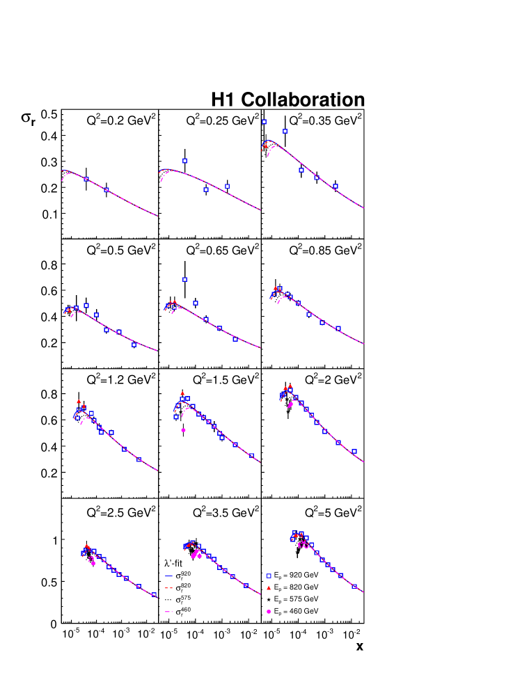
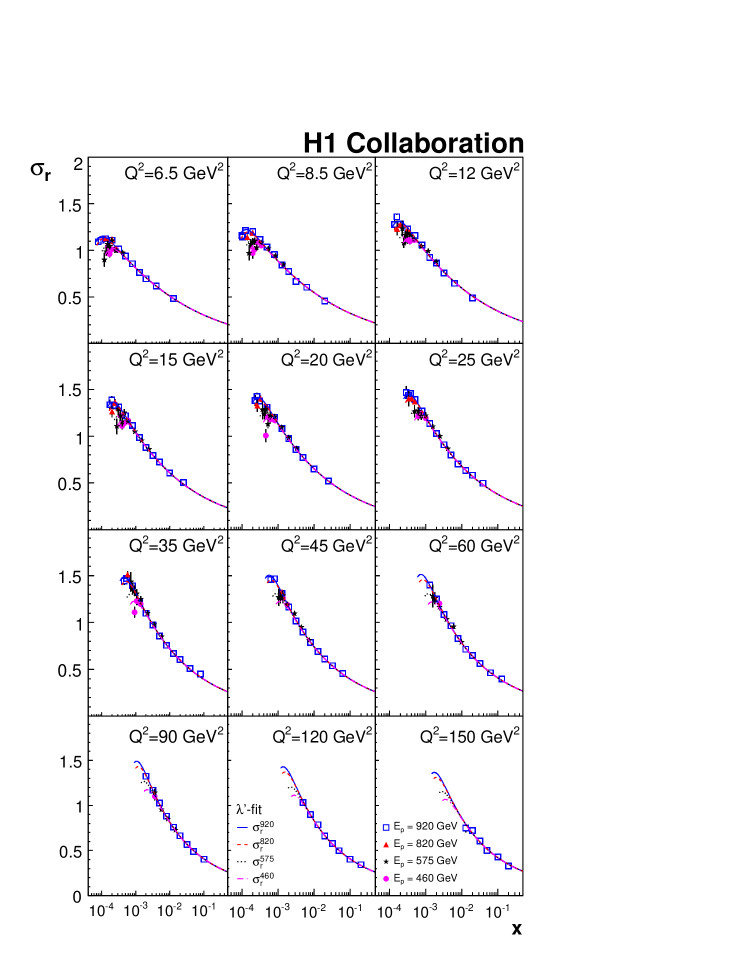
The cross-section measurements are given in tables 10-15 and shown in figure 9. The new data cover the range between GeV2 and GeV2 in reaching values of inelasticity as high as .
For the GeV sample, the new data can be compared to the previous H1 results [1, 2]. For the high region, the precision of the new data is significantly better than that of the previous H1 result, apart from the global normalisation uncertainty that is larger for the new result. This uncertainty is significantly reduced by combining the H1 measurements.
4.3 Combination of Data
For the proton beam energy , the new data cover a phase space similar to previous H1 results [1, 2] which are based on HERA-I data, collected in the years to . Therefore the data are combined, following the procedure described in [1, 52].
Four data sets are considered in this combination: the combined H1 results from HERA-I [1, 2], reported for GeV and GeV, and the two new data sets, medium CJC GeV and low BST GeV. The systematic uncertainties are assumed to be uncorrelated between the HERA-I and HERA-II measurements, apart from a overall normalisation uncertainty due to the theoretical uncertainty on the Bethe-Heitler process cross section used for the luminosity measurement. In total, there are independent sources of systematic uncertainty. For GeV2, the new data extend the kinematic coverage towards high . At low and for all values of at low , there is a sizable region of overlap.
The combined cross-section measurements are given in tables 16 to 19. The full information about correlation between cross-section measurements can be found elsewhere [53]. The data show very good compatibility, with . At low , the previous H1 data from [1, 2] have a higher precision than the new result. In particular, the global normalisation uncertainty was significantly smaller: about at HERA-I compared to at HERA-II. Therefore, in the combination, the new HERA-II data are effectively normalised to the HERA-I result and their global normalisation uncertainties are reduced significantly. Table 5 lists those few systematic sources of the HERA-II analyses, which are noticeably altered by the averaging procedure. All alterations stay within one standard deviation of the estimated error.
| Systematic Source | Shift in | Uncertainty in |
|---|---|---|
| scale | ||
The systematic errors of the HERA-I data are not significantly affected by the combination. At low , the gain in the combined data precision compared to the HERA-I result is small. The uncertainties are reduced by at most of their size and the shift of central values does not exceed . At high , however, there is a significant gain in the precision achieved by the data combination. For the region GeV2 and , for example, the accuracy of the GeV data is improved by about a factor of two. For medium , GeV2, the new high measurements, corresponding to GeV, exceed the accuracy of the HERA-I data, corresponding to GeV, by a factor to . The GeV measurement at HERA-I was limited to .
The GeV and GeV data sets are measured using an identical grid of bin centres. At low , the influence of the structure function is small. Therefore the two data sets are combined for all points satisfying after a small correction of the cross-section values to GeV. At higher the measurements are kept separately but they are affected by the combination procedure. The data show good compatibility, with , and the combined reduced cross-section values are given in tables 20 and 21. This combined reduced set, together with the combined nominal set, is used for the phenomenological analysis presented in section 6.
5 Determination of the Structure Function
5.1 Procedure
The structure function is determined using the separate GeV and GeV samples and the published GeV data from [1, 2]. To determine , common values of the grid centres are required for all centre-of-mass energies. The published GeV data have therefore been reanalysed using the binning adopted for the analysis, see table 4. To determine , the data measured at high for GeV are combined with the data at intermediate for GeV and low for GeV. The usage of the published GeV data compared to a new analysis of the HERA-II data is motivated by a wider acceptance at low , extending to GeV2. In addition, as discussed in section 4.3, adding the HERA-II data does not improve the precision at low .
The determination of the structure function depends on the treatment of the relative normalisations and systematic uncertainties of the data sets. A straightforward but simplified procedure was adopted in [17] where the data sets were normalised to each other at low . The values of the structure function were determined in straight-line fits to the reduced cross section as a function of in each bin using the statistical and uncorrelated systematic uncertainties. The correlated systematic errors were determined using an offset method. An illustration of this procedure, applied to the cross-section data from the current analysis, is shown in figure 10. The procedure adopted in [17] does not fully take into account correlations between the low and high regions, used for the cross-section normalisation and the computation. The offset method does not allow for shifts of the central values of the correlated systematic error sources. Thus the information on the goodness of the straight-line fits to the cross-section measurements at the three centre-of-mass energies is not fully employed.
The procedure for the determination is improved in the current analysis. The new method extends the averaging procedure of [1]. For additive uncertainties it is based on the minimisation of the function
| (13) |
Here is the measured central value of the reduced cross section at a point with a combined statistical and uncorrelated systematic uncertainty . The effect of correlated error sources on the cross-section measurements is approximated by the systematic error matrix . The function depends quadratically on the structure functions and ( denoted as vectors ) as well as on . Minimisation of with respect to these variables leads to a system of linear equations.
For low , the coefficient is small compared to unity and thus can not be accurately measured. In this kinematic domain, the constraint provides an even better bound on the value of than the experimental data. Furthermore, the ratio is not expected to vary strongly as a function of in the limited range of sensitivity to . For the kinematic range studied in this paper it is measured to be consistent with . To avoid unphysical values for , an extra prior is introduced for the minimisation:
| (14) |
where and the width is chosen such that it has a negligible influence for . The additional prior preserves the quadratic dependence of the function on and . The prior has a significant contribution at low only and is very similar to imposing a common cross-section normalisation at low used in [17]. Since is chosen to be large, the prior affects only points with large uncertainty on . The bias introduced by the prior is investigated by varying the value of between and and between and , and found to be negligible, for the points chosen for the determination.
5.2 Results
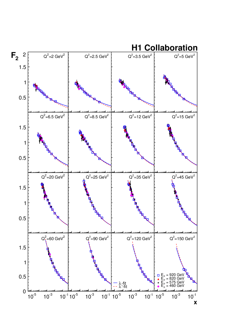
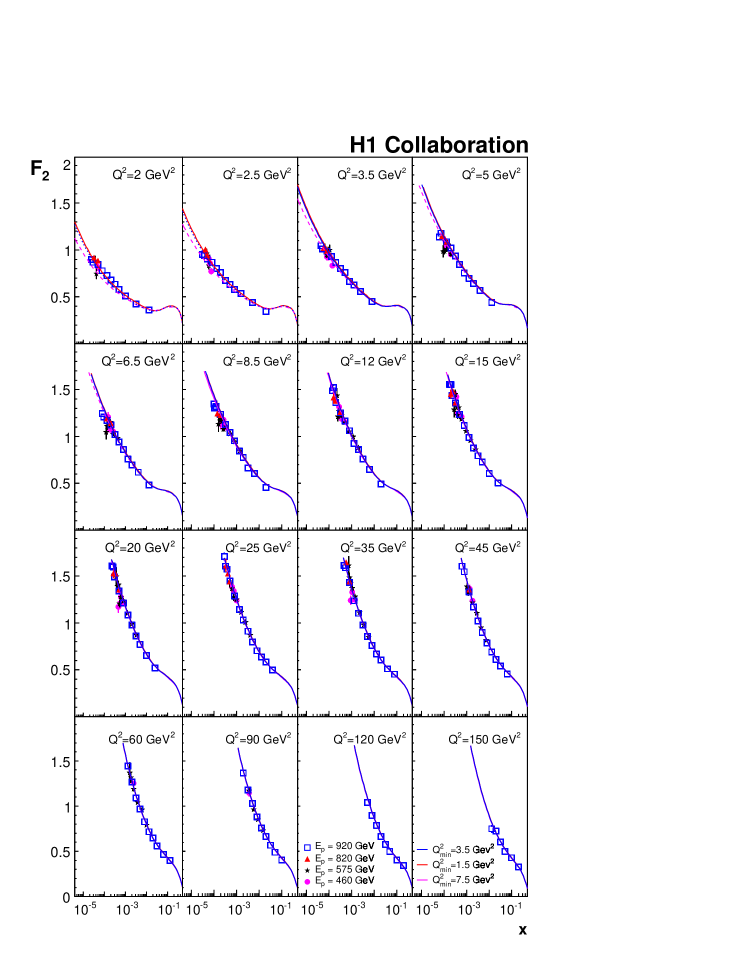
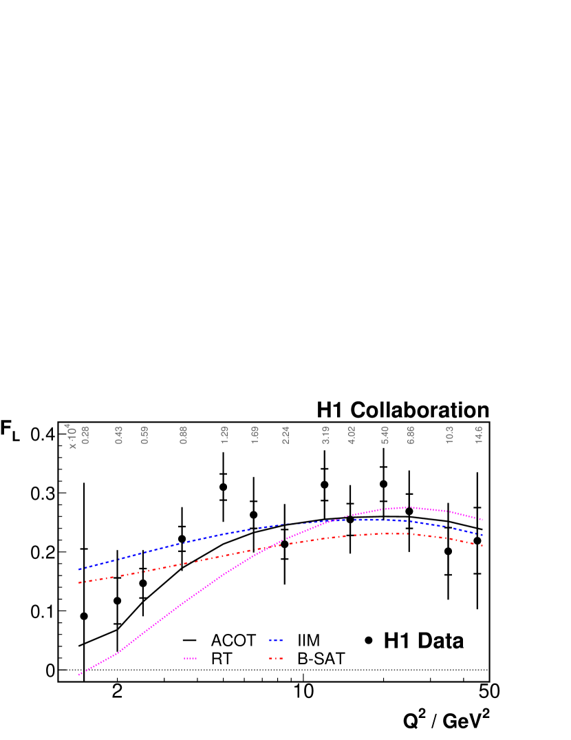
The measured structure function is given in table 22 and shown in figure 11. By convention, only measurements with total uncertainties below for GeV2 and below for GeV2 are presented. The selection on the total uncertainty removes the bias due to the prior in equation 14. The measurement spans over two decades in at low , from to . The data are compared to the result of the DGLAP ACOT fit, which is described in section 6.2. The structure function measured for the corresponding bins is given in table 22 and shown together with in figure 12. Note that compared to the previous determinations of by the H1 collaboration, this measurement represents a model independent determination without extra assumptions on .
The values of resulting from averages over at fixed are given in table 23 and presented in figure 13. The average is performed taking into account correlations. The measured structure function is compared with theoretical predictions from HERAPDF1.0 [16], CT10 [54], NNPDF2.1 [55, 56], MSTW08 [57], GJR08 [58, 59] and ABKM09 [60] sets. Depending on the PDF set, the calculations are performed at NLO or NNLO in perturbative QCD. Within the uncertainties all predictions describe the data reasonably well.
The measurement of the structure functions and can be used to determine the ratio (see equation 4). This ratio is shown in figure 14. Apart from conditions applied to select results, only measurements with total uncertainties below are included.
For GeV2, the ratio is consistent with a constant behaviour. This hypothesis is tested by a simultaneous determination of the values of the structure function at all data points under the assumption that is constant. In this procedure, values of are scanned between and in steps, and each of the cross-section measurements is used to calculate the structure function using equation 5. The measurements of from different are then combined using the standard averaging programme [1] taking into account correlations of the systematic uncertainties. Figure 15 shows the results of this scan represented as for each average as a function of . The minimum is found at where suggesting a conservative error estimation. It is remarkable that all the low , low GeV2 data are consistent with the hypothesis that is constant.
6 Phenomenological Analysis
The combined cross-section data for and GeV are used for several phenomenological analyses. The fits are applied to the combined reduced cross-section measurements accounting for correlations between the data points.
In the following, the quality of different fits is compared in terms of . Since the systematic uncertainties dominate over statistics, and they are estimated conservatively, in several cases is observed to be less than unity. This, however, does not prevent the comparison of quality among different fits with the same number of degrees of freedom in terms of since the average error overestimation, approximated as , does not exceed .
6.1 Fit
The increase of the structure function for can be approximated by a power law in , . This simple parameterisation was shown to describe previous H1 data rather well for [18]. In the recent H1 analysis [1], a fit was performed to the measured reduced cross section, , represented as
| (15) |
by allowing to float for each bin independently. At low GeV2, this lead to surprisingly large values of , which are incompatible with the result obtained in section 5.2. A similar behaviour is observed when equation 15 is applied to the present data. This points to some inconsistency in the simple power law for the rise of towards low and the measured value of . A different approach is therefore adopted in this analysis. It is generally assumed that for all bins. A fit termed the fit is made with only and as free parameters. This is extended in a subsequent step to allow for possible deviations in the behaviour of from the simple fit formula.
The combined H1 data are fitted using the offset method to evaluate systematic uncertainties. The parameters obtained in the fits as a function of are shown in figure 16. The parameter exhibits an approximately linear increase as a function of for GeV2. For lower , the variation of deviates from that linear dependence. The normalisation coefficient rises with increasing for GeV2 and is consistent with a constant behaviour for higher , as in [18]. The total of the fit is when the uncertainties are taken as the statistical and uncorrelated systematic uncertainties added in quadrature. Values of significantly larger than unity may arise in the offset method because it does not take into account the correlated systematic uncertainties. Studies show that the largest contribution to the arises from the GeV2 domain. In order to further investigate this behaviour, the parameterisation of the structure function is extended by one additional parameter
| (16) |
to allow for deviations from a single power law. This fit returns a significantly improved . The parameters and are shown in figure 17. From this figure, it is interesting to observe that the parameter becomes consistent with having a constant value of . The two parameters and are strongly correlated since for each bin the data span over a limited range in . Therefore, fits are performed, termed fits, for which is fixed. The quality of these fits with a total is better than of the original fits. The fitted parameters and are shown in figure 18. A comparison of the fit result with the H1 reduced cross-section data is given in figures 19 and 20. Figure 21 shows comparison of the and fits for GeV2 with the structure function which is calculated from the reduced cross sections assuming . The parameter is negative and shows a constant behaviour for GeV2, with a smooth transition and a linear rise with for GeV2. Therefore, for the low domain, the fit shows somewhat softer increase towards low compared to the fit opposite to that observed for higher values. The present measurement of therefore leads to a refined understanding of the rise of towards low , which appears to be tamed at low , and correspondingly lower , compared to a pure power-law behaviour, as it was predicted in [61].
In order to consolidate the observations obtained with the offset method, an analysis is performed in which the errors are evaluated using the Hessian method following the definition given in [2]. The fitted parameters are coefficients or for the bins and the parameters for the sources of the systematic uncertainty. The fit returns compared to a worse of the fit.
6.2 DGLAP Fit
The new combined H1 data are used together with the previously published high GeV2 H1 data [4, 5, 6] as input to a DGLAP pQCD fit analysis to NLO, with the main objective of studying predictions. The HERA measurement regions are limited by GeV2 and , such that target mass corrections and higher twist contributions can be assumed to be small. In addition, in order to restrict to a region where perturbative QCD is valid, only data with GeV2 are used in the central fit. The influence of this value is discussed further in this section. The internal consistency of the input data set enables a calculation of the experimental uncertainties on the PDFs using the tolerance criterion of . The data are fitted using the program QCDNUM [62] and the complete error correlation information in a fit as in [2] using MINUIT [63] as the minimisation program.
The fit procedure begins with parameterising the input parton distribution functions (PDFs) at a starting scale , chosen to be below the charm mass threshold. The PDFs are then evolved using the DGLAP evolution equations [24, 25, 26, 27, 28] at NLO [29, 30] in the scheme with the renormalisation and factorisation scales set to , and the strong coupling to [64]. The QCD predictions for the structure functions are obtained by convoluting the PDFs with the calculable NLO coefficient functions. Those are calculated using the general mass variable-flavour scheme of ACOT [33] and cross checked against the RT scheme [31, 32]. The ACOT and RT schemes differ in the inclusion of various terms at higher orders in for the computation of the heavy quark structure functions, and for the structure function .
For the QCD fit, the following independent input PDFs are chosen: the valence quark distributions and , the gluon distribution and anti-quark distributions and . The conditions , and are imposed at the starting scale . A standard generic functional form is used to parameterise these PDFs:
| (17) |
The normalisation parameters, and , are constrained by the fermion number and momentum sum rules. The up and down quark type parameters are set equal, , such that there is only a single parameter for the sea distributions, which governs the PDFs at low .
The strange quark distribution is already present at the starting scale, and it is assumed that at . The strange fraction is chosen to be , which is consistent with determinations of this fraction using neutrino induced di-muon production data [57, 65]. In addition, to ensure that as , the constraint is applied.
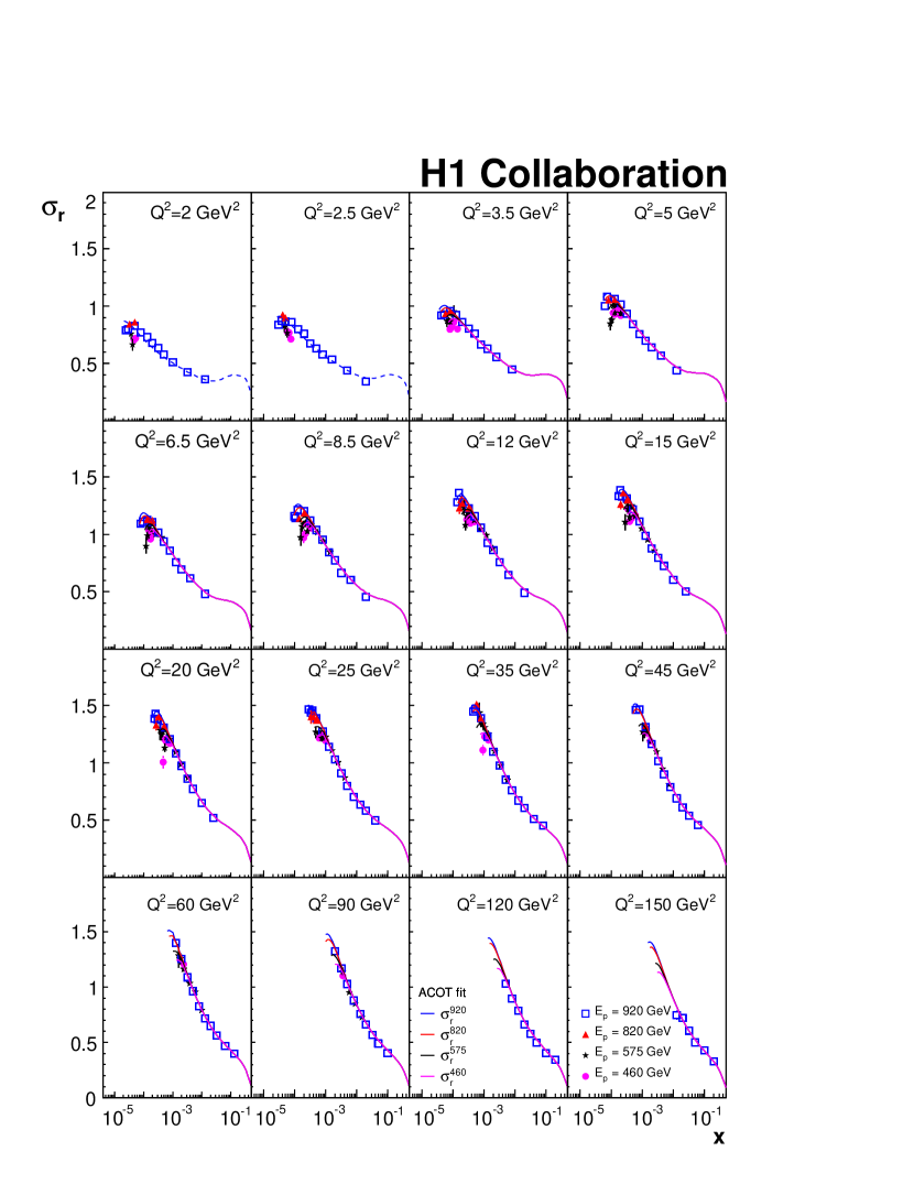
The initial fits are performed using the same parameterisation type as for the HERAPDF1.0 fit [16], which has only one free polynomial parameter, . For this parameterisation, the ACOT and RT heavy flavour schemes are compared. Both fits give good descriptions of the data, but the ACOT fit, which has , is superior to the RT fit, with , by about units. Therefore, the ACOT fit is chosen for further more detailed investigations.
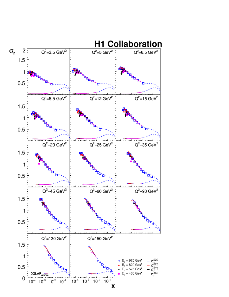
The central fit is chosen in a optimisation procedure, as previously used by H1 [2], in which all extra parameters are first set to zero, leading to a nine parameter fit. They are then added, one at a time until no significant improvement in is observed. In addition, the assumption that is removed and a flexible parameterisation for the gluon density with two extra parameters [16] is also tried but both variations do not lead to significant fit improvements. The parameterisation procedure also requires for the central fit that all PDFs are positive definite. The best fit is obtained with the extra free parameters and resulting in a . Figure 22 compares the fit result to the low H1 data. As a consistency check, a fit using the RT heavy flavour scheme is repeated. A similar increase in of about units is observed in this case.
| / GeV2 | ||||||
|---|---|---|---|---|---|---|
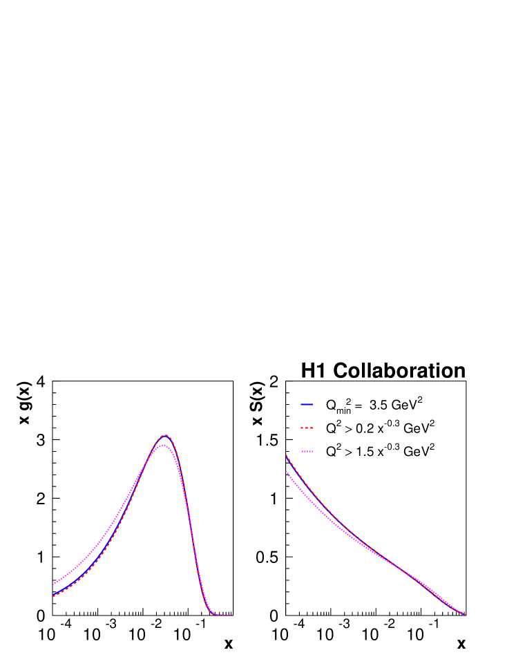
The sensitivity of the fit to the inclusion of low data is studied by varying the cut. The variation of the fit quality in terms of is summarised in table 6. Increasing the cut leads to a steady decrease in the , suggesting that the fit has some difficulties to describe the data at low values. Figure 23 compares the structure function with the fits performed using different cuts. At low the shape of the measured structure function as a function of is somewhat different from those obtained by the DGLAP fits based on the parameterisation described above. The fit obtained with a cut of GeV2 falls significantly below the data at small when extrapolating to the low region. Figure 24 shows gluon and sea-quark distributions for different values of at the evolution starting scale GeV2. A change of from GeV2 to GeV2 leads to an increase of the gluon distribution while the sea-quark distribution becomes smaller at low . This suppression of the sea-quark contribution at small when using a cut of GeV2 is responsible for the smaller values of obtained by this fit at small and small .
An alternative approach to the variation is a saturation-inspired cut on the kinematic region depending on like
| (18) |
with and different values of the parameter , as suggested in [66]. The dependence of on is given in table 7. Figure 25 shows gluon and sea-quark distributions for different values of . The saturation-inspired cut has an effect similar to the one of the variation. The fit quality improves with increasing and the gluon becomes larger while the sea-quark density decreases at low .
To facilitate the comparison of the data with dipole model predictions, DGLAP fits are also performed in the kinematic domain and GeV2, in which both the DGLAP theory and the dipole ansatz can be assumed to hold. The valence quark parameters cannot be determined in this range. Therefore they are fixed to the values obtained by the full phase space fits. There are six non-valence quark parameters, , , , , and , as compared to three free parameters of the dipole models discussed below. When restricted to this common kinematic domain, the ACOT fit is of very good quality, with while the RT fit yields .
6.3 Dipole Model Fits
At low and low , virtual photon-proton scattering has been described using the colour dipole model [19]. In this model, the scattering process is calculated as a fluctuation of the photon into a quark-antiquark pair (dipole), with a lifetime , which interacts with the proton.
Several approaches were developed to phenomenologically describe the dipole-proton interaction cross section, three of which are subsequently applied to the data of this paper. These are the original model version (GBW) [20], a model based on the colour glass condensate approach to the high parton density regime (IIM) [21], and a model with the generalised impact parameter dipole saturation (B-SAT) [22].
In the GBW model the dipole-proton cross section is given by
| (19) |
where corresponds to the transverse separation between the quark and the antiquark, and is an dependent scale parameter, assumed to have the form
| (20) |
The parameters of the fit are the cross-section normalisation as well as and . The IIM model has a modified expression for using the parameter instead of . The B-SAT model modifies equation 19 by adding effects of the DGLAP evolution. This model uses as an input a gluon density
| (21) |
with the starting scale , normalisation and low exponent as free parameters while the other dipole model parameters are kept fixed.
The dipole models are applicable at low where the gluon and sea quark densities dominate. The models are valid down to the photoproduction limit , therefore no cut is applied for the central fits. In DGLAP fits it is observed that the contribution of the valence quarks to the scattering cross section is sizeable for the whole HERA kinematic range, compared to the data precision. This contribution varies between and for varying from to . Modified dipole fits are therefore performed, in which the contribution from the valence quarks to the cross section, as determined by the central DGLAP fit, is added to the dipole model prediction. These fits are performed requiring that GeV2, to be consistent with DGLAP analyses.
It should be noted that the size of the valence-quark contribution at low is rather uncertain because it is only indirectly constrained by the HERA data. For it is determinedned by the combination of neutral and charged current scattering cross sections measurements. At lower however the valence quark contribution follows from the parameterisation and the fermion number sum rules. The uncertainty can reach at [16].
| Parameter | Value | Uncertainty | Value | Uncertainty | Value | Uncertainty |
|---|---|---|---|---|---|---|
| Nominal GBW | GeV2 GBW | GBW+DGLAPvalence | ||||
| (mb) | ||||||
| Nominal IIM | GeV2 IIM | IIM+DGLAPvalence | ||||
| (fm) | ||||||
| Nominal B-SAT | GeV2 B-SAT | B-SAT+DGLAPvalence | ||||
| (GeV2) | ||||||
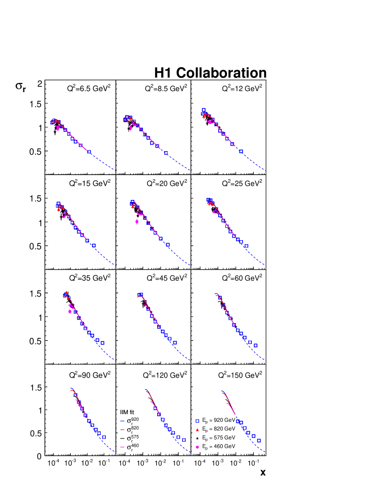
Dipole models fits are performed using the same minimisation package as for the DGLAP fit. The values of parameters and their uncertainties are estimated using a Monte Carlo method [67]111The Monte Carlo method is preferred for the estimation of uncertainties compared to the MINUIT error estimation in order to avoid instabilities of numerical integration used in the Dipole codes.. The parameters of the fits are given in table 8. The fit qualities are summarised together with the results obtained for DGLAP fits in table 9. Among the dipole models, the IIM fit provides the best description of the data. It is shown in figures 26 and 27. The B-SAT model, which includes some DGLAP evolution, provides a worse fit to the data yet still with an acceptable . The GBW model, however, fails to describe the data. This fit agrees with the data well at low , but falls significantly below the data for GeV2, where the DGLAP evolution, neglected in the model, plays an important role. Fits with a DGLAP-based correction for the contribution of the valence quarks are restricted to GeV2. In order to simplify comparisons, pure dipole model fits with the same cut are performed too. The addition of the valence-quark contribution allows an acceptable description of the data at high , however, the overall fit quality is reduced. The fitted parameters of the models vary beyond their experimental uncertainties. As an example, a comparison of the reduced cross-section data to the IIM+DGLAPvalence fit is given in figure 28.
Finally, the fits at and GeV2 are compared in terms of for the three dipole and two DGLAP models (table 9). The best description is obtained with the ACOT fit, followed by the pure dipole model IIM and B-SAT fits. The DGLAP RT fit is of similar quality as the IIM+DGLAPvalence fit, followed by the B-SAT+DGLAPvalence fit. The GBW fit fails to describe the data in this kinematic domain.
In both the DGLAP and the dipole models the structure function can be calculated once the model parameters are fixed. It is thus of interest to compare the predictions of the different models with the data, which is illustrated in figure 29. For high GeV2, all models agree with the data and with each other well. For lower values, there is a significant difference between the predictions. The DGLAP fit in the RT scheme predicts low values of , while in the DGLAP fit in the ACOT scheme the decrease of occurs at lower values of . The predictions of the dipol models considered here show only little variation with . All predictions, except the DGLAP RT fit, agree with the data well. The dependence of is best reproduced by the DGLAP ACOT fit.
| Fit Conditions | GBW | IIM | B-SAT | ACOT | RT |
|---|---|---|---|---|---|
| Nominal fit | |||||
| GeV2 | |||||
| DGLAPvalence | |||||
7 Summary
A measurement is presented of the inclusive double differential cross section for neutral current deep inelastic scattering at small Bjorken and low absolute four-momentum transfers squared, . The measurement extends to high values of inelasticity . The data were collected with the H1 detector for the proton beam energy of GeV, in the years to , and for GeV and GeV, in . The integrated luminosities of the measurements are pb-1, pb-1 and pb-1 for the GeV, GeV and GeV data samples, respectively. The data at GeV significantly improve the accuracy of the cross-section measurements at high when compared to the previous H1 data. All data are combined with the HERA-I results to provide a new accurate data sample covering GeV2, and which supersedes previous H1 measurements of the DIS cross section and of in this kinematic domain.
The data at GeV and GeV, together with the measurements at GeV are used to determine the structure function . This extraction applies a novel method which takes into account the correlations of data points due to systematic uncertainties. This is the first measurement at low GeV2 and , which became possible by employing a dedicated backward silicon tracker for the electron reconstruction. The data are reasonably well reproduced by the predictions based on NLO and NNLO QCD.
The measurements of are used to determine the ratio . For GeV2, the ratio shows a constant behaviour with .
The combined H1 data are subjected to phenomenological analyses. The rise of the structure function towards low is examined using power-law fits. As in previous H1 analyses, the power-law exponent is found to be approximately constant for GeV2 but increases linearly with for higher values. Closer inspection of the fits reveals, however, a deterioration of the fit quality for the GeV2 range. A parameterisation which allows for a dependent correction to a fixed power-law, for , provides an improved description of the data with the same number of parameters. This observation suggests that the dependence of the structure function may deviate from a simple power law at small and small exhibiting a softer rise. This confirms a QCD prediction of [61], according to which the rise of should be slower than any power of but faster than any power of .
The data are found to be well described by an NLO DGLAP QCD analysis. The ACOT and the RT schemes are used, which differ in the treatment of the heavy-flavour and higher-order contributions to the cross section. A comparison of ACOT and RT based fits to the data reveals a significant preference for the ACOT treatment.
The sensitivity of the DGLAP fits to low and low effects is checked by varying the of the data and also by applying a saturation-model inspired [66] selection of the data. While for all variants of the cuts the fits provide a good description of the data, the fit quality improves as more data at low and low are removed from the analysis. This also leads to an increase of the gluon and a decrease of the sea-quark densities at low .
Dipole model based analyses are applied to the data at using three variants of them. The GBW model is unable to describe the data at larger , while the IIM and B-SAT models agreed with the data generally well. The influence of valence quarks at low is investigated by adding their contribution as estimated from the ACOT fit. These models together with the two DGLAP fits are compared to each other by fitting the data in a common kinematic range. The DGLAP ACOT fit provides the best description of the data, followed closely by the dipole IIM and B-SAT models. All models agree well with the measurement at GeV2. For lower , however, the RT fit falls significantly below the data while the other models describe the measured well.
The present measurement and the combination with all accurate H1 DIS cross section data provide a total cross section uncertainty of about % at low and low . The structure function rises towards low . The structure function is measured directly. Both structure functions agree with pQCD expectations.
Acknowledgements
We are grateful to the HERA machine group whose outstanding efforts have made this experiment possible. We thank the engineers and technicians for their work in constructing and maintaining the H1 detector, our funding agencies for financial support, the DESY technical staff for continual assistance and the DESY directorate for support and for the hospitality which they extend to the non-DESY members of the collaboration.
References
- Aaron et al. [2009a] F. Aaron et al. [H1 Collaboration], Eur. Phys. J. C63, 625 (2009w) [arXiv:0904.0929].
- Aaron et al. [2009b] F. Aaron et al. [H1 Collaboration], Eur. Phys. J. C64, 561 (2009w) [arXiv:0904.3513].
- Adloff et al. [2001a] C. Adloff et al. [H1 Collaboration], Eur. Phys. J. C21, 33 (2001w) [hep-ex/0012053].
- Adloff et al. [2000] C. Adloff et al. [H1 Collaboration], Eur. Phys. J. C13, 609 (2000) [hep-ex/9908059].
- Adloff et al. [2001b] C. Adloff et al. [H1 Collaboration], Eur. Phys. J. C19, 269 (2001w) [hep-ex/0012052].
- Adloff et al. [2003] C. Adloff et al. [H1 Collaboration], Eur. Phys. J. C 30, 1 (2003) [hep-ex/0304003].
- Breitweg et al. [1997] J. Breitweg et al. [ZEUS Collaboration], Phys. Lett. B407, 432 (1997) [hep-ex/9707025].
- Breitweg et al. [2000a] J. Breitweg et al. [ZEUS Collaboration], Phys. Lett. B 487, 53 (2000w) [hep-ex/0005018].
- Breitweg et al. [1999] J. Breitweg et al. [ZEUS Collaboration], Eur. Phys. J. C7, 609 (1999) [hep-ex/9809005].
- Chekanov et al. [2001] S. Chekanov et al. [ZEUS Collaboration], Eur. Phys. J. C 21, 443 (2001) [hep-ex/0105090].
- Breitweg et al. [2000b] J. Breitweg et al. [ZEUS Collaboration], Eur. Phys. J. C 12, 411 (2000w) [Erratum-ibid. C27 (2003) 305] [hep-ex/9907010].
- Chekanov et al. [2003a] S. Chekanov et al. [ZEUS Collaboration], Eur. Phys. J. C28, 175 (2003w) [hep-ex/0208040].
- Chekanov et al. [2002] S. Chekanov et al. [ZEUS Collaboration], Phys. Lett. B539, 197 (2002), [Erratum-ibid. B552 (2003) 308] [hep-ex/0205091].
- Chekanov et al. [2004] S. Chekanov et al. [ZEUS Collaboration], Phys. Rev. D 70, 052001 (2004) [hep-ex/0401003].
- Chekanov et al. [2003b] S. Chekanov et al. [ZEUS Collaboration], Eur. Phys. J. C32, 1 (2003w) [hep-ex/0307043].
- Aaron et al. [2010] F. Aaron et al. [H1 and ZEUS Collaborations], JHEP 1001, 109 (2010) [arXiv:0911.0884].
- Aaron et al. [2008] F. Aaron et al. [H1 Collaboration], Phys. Lett. B665, 139 (2008) [arXiv:0805.2809].
- Adloff et al. [2001c] C. Adloff et al. [H1 Collaboration], Phys. Lett. B520, 183 (2001w) [hep-ex/0108035].
- Nikolaev and Zakharov [1991] N. N. Nikolaev and B. G. Zakharov, Z. Phys. C 49, 607 (1991).
- Golec-Biernat and Wüsthoff [1999] K. Golec-Biernat and M. Wüsthoff, Phys. Rev. D 59, 014017 (1999) [hep-ph/9807513].
- Iancu et al. [2004] E. Iancu, K. Itakura, and S. Munier, Phys. Lett. B590, 199 (2004) [hep-ph/0310338].
- Kowalski et al. [2006] H. Kowalski, L. Motyka, and G. Watt, Phys. Rev. D 74, 074016 (2006) [hep-ph/0606272].
- Albacete et al. [2009] J. L. Albacete, N. Armesto, J. G. Milhano, and C. A. Salgado, Phys. Rev. D80, 034031 (2009) [arXiv:0902.1112].
- Gribov and Lipatov [1972a] V. N. Gribov and L. N. Lipatov, Sov. J. Nucl. Phys. 15, 438 (1972a).
- Gribov and Lipatov [1972b] V. N. Gribov and L. N. Lipatov, Sov. J. Nucl. Phys. 15, 675 (1972b).
- Lipatov [1975] L. N. Lipatov, Sov. J. Nucl. Phys. 20, 94 (1975).
- Dokshitzer [1977] Y. L. Dokshitzer, Sov. Phys. JETP 46, 641 (1977).
- Altarelli and Parisi [1977] G. Altarelli and G. Parisi, Nucl. Phys. B 126, 298 (1977).
- Curci et al. [1980] G. Curci, W. Furmanski, and R. Petronzio, Nucl.Phys. B175, 27 (1980).
- Furmanski and Petronzio [1980] W. Furmanski and R. Petronzio, Phys.Lett. B97, 437 (1980).
- Thorne and Roberts [1998] R. S. Thorne and R. G. Roberts, Phys. Rev. D 57, 6871 (1998) [hep-ph/9709442].
- Thorne [2006] R. S. Thorne, Phys. Rev. D73, 054019 (2006) [hep-ph/0601245].
- Kramer et al. [2000] M. Kramer, F. I. Olness, and D. E. Soper, Phys. Rev. D62, 096007 (2000) [hep-ph/0003035].
- Abt et al. [1997a] I. Abt et al. [H1 Collaboration], Nucl. Instr. and Meth. A 386, 310 (1997a).
- Abt et al. [1997b] I. Abt et al. [H1 Collaboration], Nucl. Instr. and Meth. A 386, 348 (1997b).
- Appuhn et al. [1997] R. D. Appuhn et al. [H1 SpaCal Group], Nucl. Instr. and Meth. A 386, 397 (1997).
- Andrieu et al. [1993a] B. Andrieu et al. [H1 Calorimeter Group], Nucl. Instrum. Meth. A336, 460 (1993a).
- Barwolff et al. [1989] H. Barwolff et al., Nucl. Instrum. Meth. A283, 467 (1989).
- Becker et al. [2008] J. Becker et al., Nucl. Instrum. Meth. A586, 190 (2008).
- Pitzl et al. [2000] D. Pitzl et al., Nucl. Instr. and Meth. A 454, 334 (2000) [hep-ex/0002044].
- Eick et al. [1997] W. Eick et al., Nucl. Instr. and Meth. A 386, 81 (1997).
- Andrieu et al. [1993b] B. Andrieu et al. [H1 Calorimeter Group], Nucl. Instrum. Meth. A336, 499 (1993b).
- Schuler and Spiesberger [1991] G. A. Schuler and H. Spiesberger, in Physics at HERA, vol. 3, edited by W. Buchmüller and G. Ingelman (1991), pp. 1419–1432, DJANGOH 1.4.
- Courau and Kessler [1992] A. Courau and P. Kessler, Phys. Rev. D46, 117 (1992), COMPTON 2.2.
- Kwiatkowski et al. [1992] A. Kwiatkowski, H. Spiesberger, and H.-J. Moehring, Comp. Phys. Comm. 69, 155 (1992).
- Arbuzov et al. [1996] A. Arbuzov et al., Comp. Phys. Comm. 94, 128 (1996), HECTOR 1.0 [hep-ph/9511434].
- Brun et al. [1987] R. Brun et al., GEANT3 User’s Guide, CERN (1987) [CERN-DD/EE 84-01].
- Grindhammer et al. [1990] G. Grindhammer, M. Rudowicz, and S. Peters, Nucl. Instr. and Meth. A 290, 469 (1990).
- Glazov et al. [2010a] A. Glazov, N. Raicevic, and A. Zhokin, Comput. Phys. Commun. 181, 1008 (2010a).
- Piec [2009] S. Piec, Doctoral thesis, Humboldt-Universität zu Berlin (2009), [http://www-h1.desy.de/psfiles/theses/h1th-546.pdf].
- Blobel and Kleinwort [2002] V. Blobel and C. Kleinwort, A new method for the high precision alignment of track detectors (2002) [hep-ex/0208021].
- Glazov [2005] A. Glazov, AIP Conf. Proc. 792, 237 (2005).
- [53] Correlation information can be found at https://www.desy.de/h1/.
- Lai et al. [2010] H.-L. Lai et al., Phys. Rev. D82, 074024 (2010) [arXiv:1007.2241].
- Ball et al. [2010] R. D. Ball et al., Nucl. Phys. B838, 136 (2010), [arXiv:1002.4407].
- Forte et al. [2010] S. Forte, E. Laenen, P. Nason, and J. Rojo, Nucl. Phys. B834, 116 (2010) [arXiv:1001.2312].
- Martin et al. [2009] A. D. Martin, W. J. Stirling, R. S. Thorne, and G. Watt (2009) [arXiv:0901.0002].
- Gluck et al. [2008a] M. Gluck, P. Jimenez-Delgado, and E. Reya, Eur. Phys. J. C53, 355 (2008w) [arXiv:0709.0614].
- Gluck et al. [2008b] M. Gluck, P. Jimenez-Delgado, E. Reya, and C. Schuck, Phys. Lett. B664, 133 (2008w) [arXiv:0801.3618].
- Alekhin et al. [2010] S. Alekhin, J. Blumlein, S. Klein, and S. Moch, Phys. Rev. D81, 014032 (2010) [arXiv:0908.2766].
- De Rujula et al. [1974] A. De Rujula et al., Phys. Rev. D10, 1649 (1974).
- Botje [2010] M. Botje (2010), http://www.nikef.nl/h24/qcdnum/index.html [arXiv:1005.1481].
- James and Roos [1975] F. James and M. Roos, Comput. Phys. Commun. 10, 343 (1975).
- C. Amsler et al. (2008) [Particle Data Group] C. Amsler et al. (Particle Data Group), Phys. Lett. B667, 1 (2008).
- Nadolsky et al. [2008] P. M. Nadolsky et al., Phys. Rev. D78, 013004 (2008) [arXiv:0802.0007].
- Caola et al. [2010] F. Caola, S. Forte, and J. Rojo, Phys. Lett. B686, 127 (2010) [arXiv:0910.3143].
- Glazov et al. [2010b] A. Glazov, S. Moch, and V. Radescu, Accepted by Phys. Lett. B doi:10.1016/j.physletb.2003.10.071 (2010w) [arXiv:1009.6170].
| GeV2 | % | % | % | % | % | % | % | % | |||
|---|---|---|---|---|---|---|---|---|---|---|---|
| GeV2 | % | % | % | % | % | % | % | % | |||
|---|---|---|---|---|---|---|---|---|---|---|---|
| GeV2 | % | % | % | % | % | % | % | % | % | |||
|---|---|---|---|---|---|---|---|---|---|---|---|---|
| GeV2 | % | % | % | % | % | % | % | % | % | |||
|---|---|---|---|---|---|---|---|---|---|---|---|---|
| GeV2 | % | % | % | % | % | % | % | % | % | |||
|---|---|---|---|---|---|---|---|---|---|---|---|---|
| GeV2 | % | % | % | % | % | % | % | % | % | |||
|---|---|---|---|---|---|---|---|---|---|---|---|---|
| Bin | ||||||||||
|---|---|---|---|---|---|---|---|---|---|---|
| GeV2 | % | % | % | % | GeV | |||||
| Bin | ||||||||||
|---|---|---|---|---|---|---|---|---|---|---|
| GeV2 | % | % | % | % | GeV | |||||
| Bin | ||||||||||
|---|---|---|---|---|---|---|---|---|---|---|
| GeV2 | % | % | % | % | GeV | |||||
| Bin | ||||||||||
|---|---|---|---|---|---|---|---|---|---|---|
| GeV2 | % | % | % | % | GeV | |||||
| Bin | ||||||||||
|---|---|---|---|---|---|---|---|---|---|---|
| GeV2 | % | % | % | % | GeV | |||||
| Bin | ||||||||||
|---|---|---|---|---|---|---|---|---|---|---|
| GeV2 | % | % | % | % | GeV | |||||
| GeV2 | ||||||
|---|---|---|---|---|---|---|
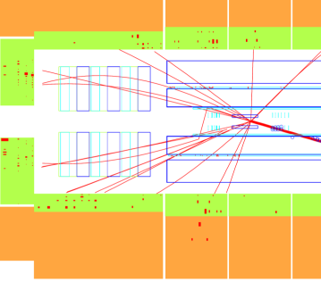
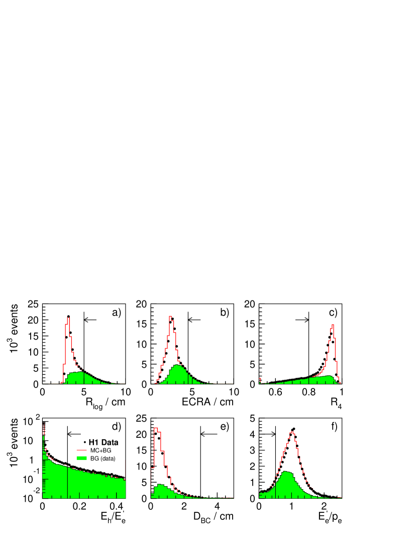


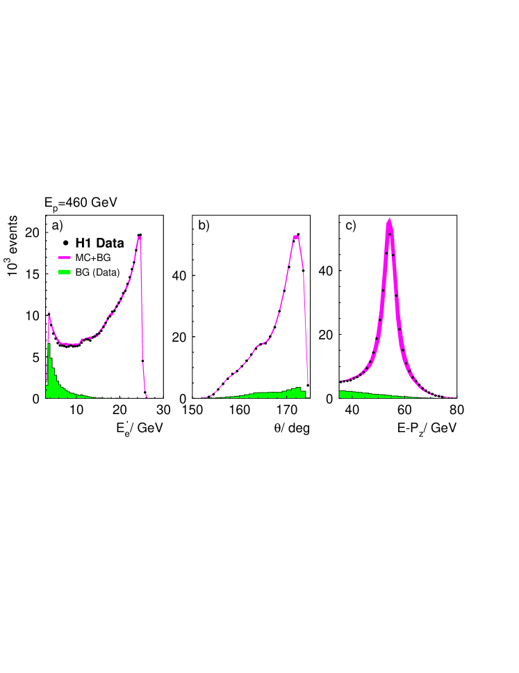
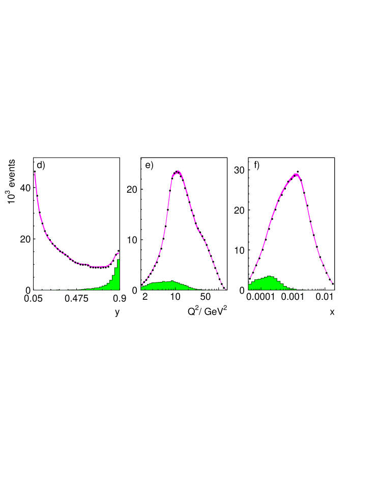
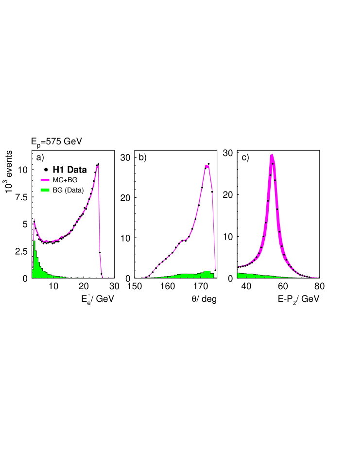
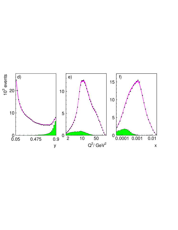
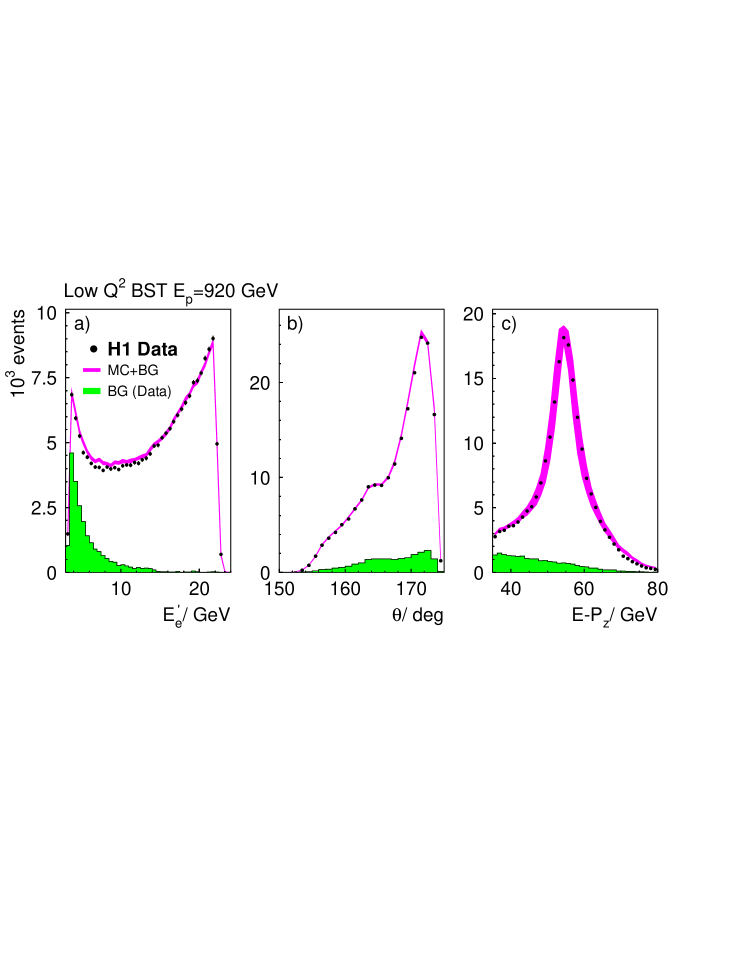
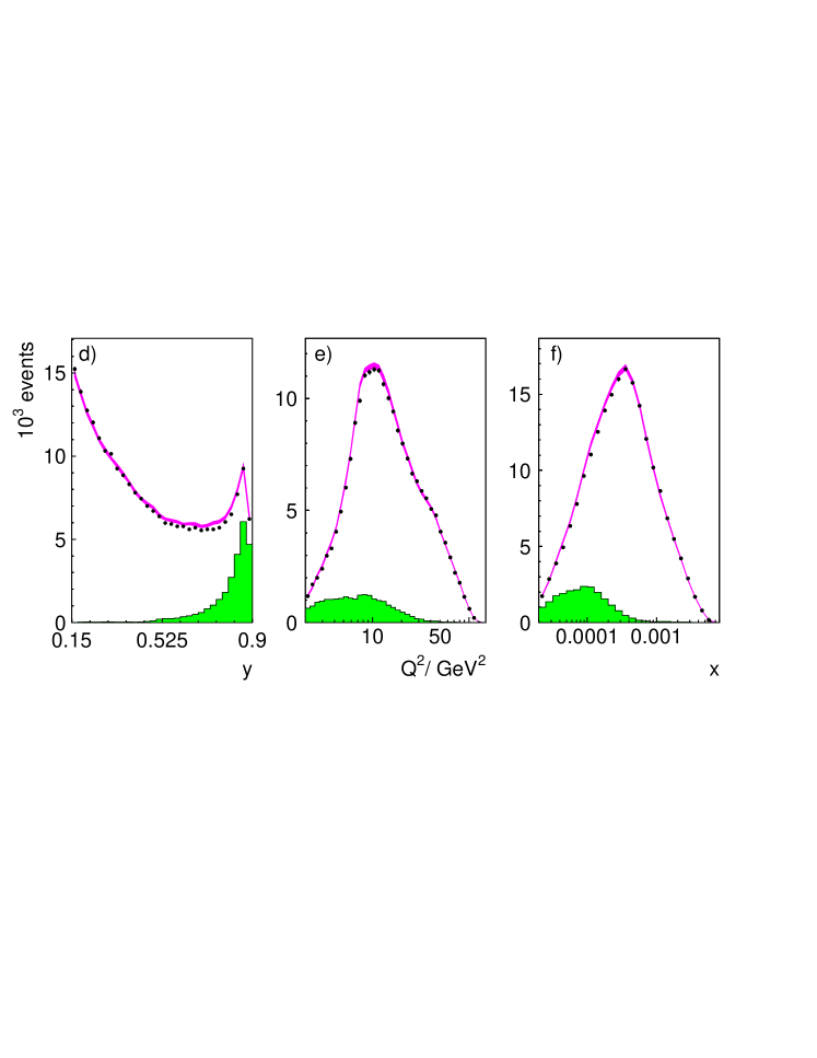
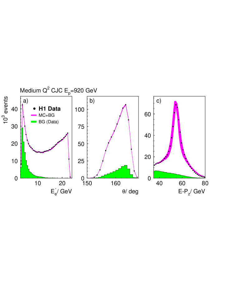
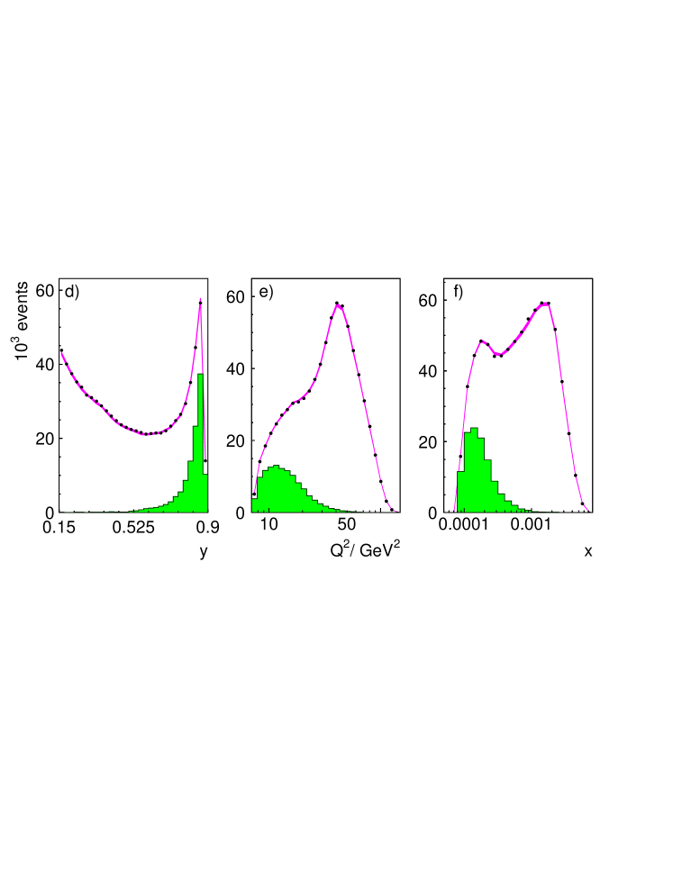
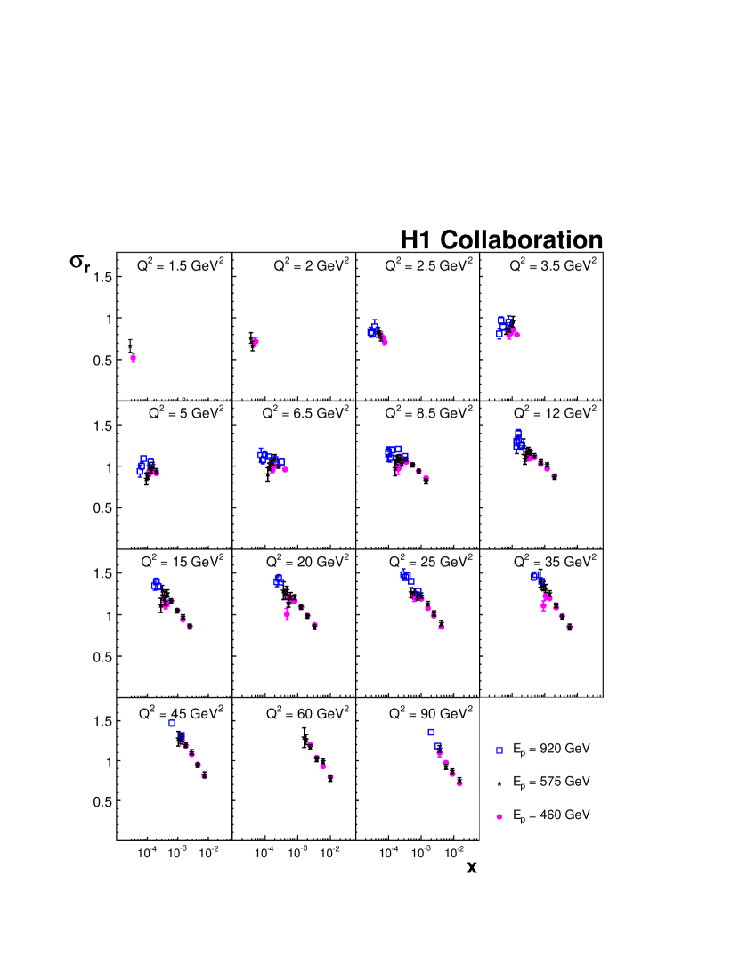
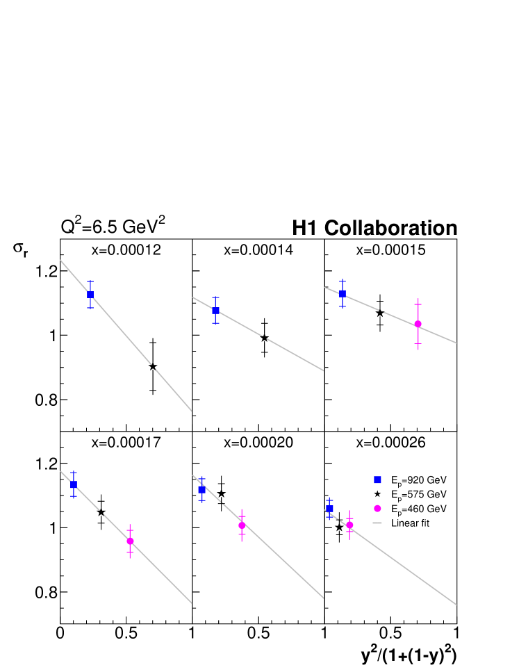
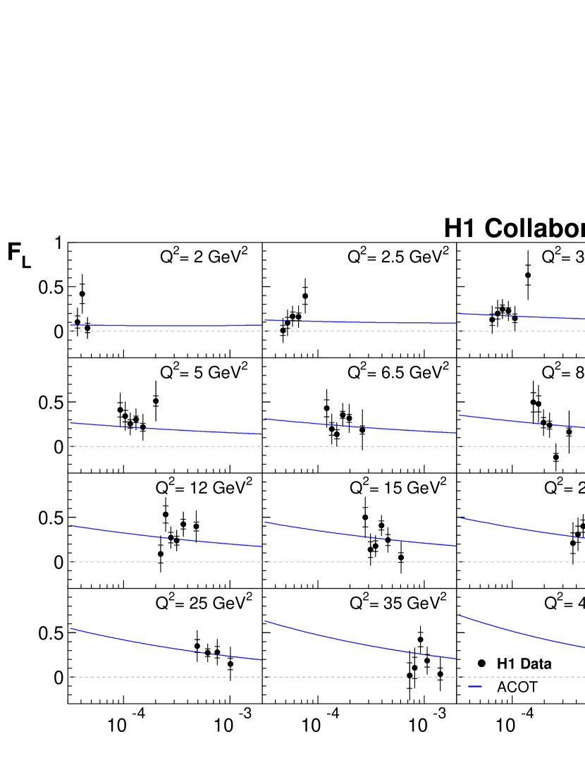
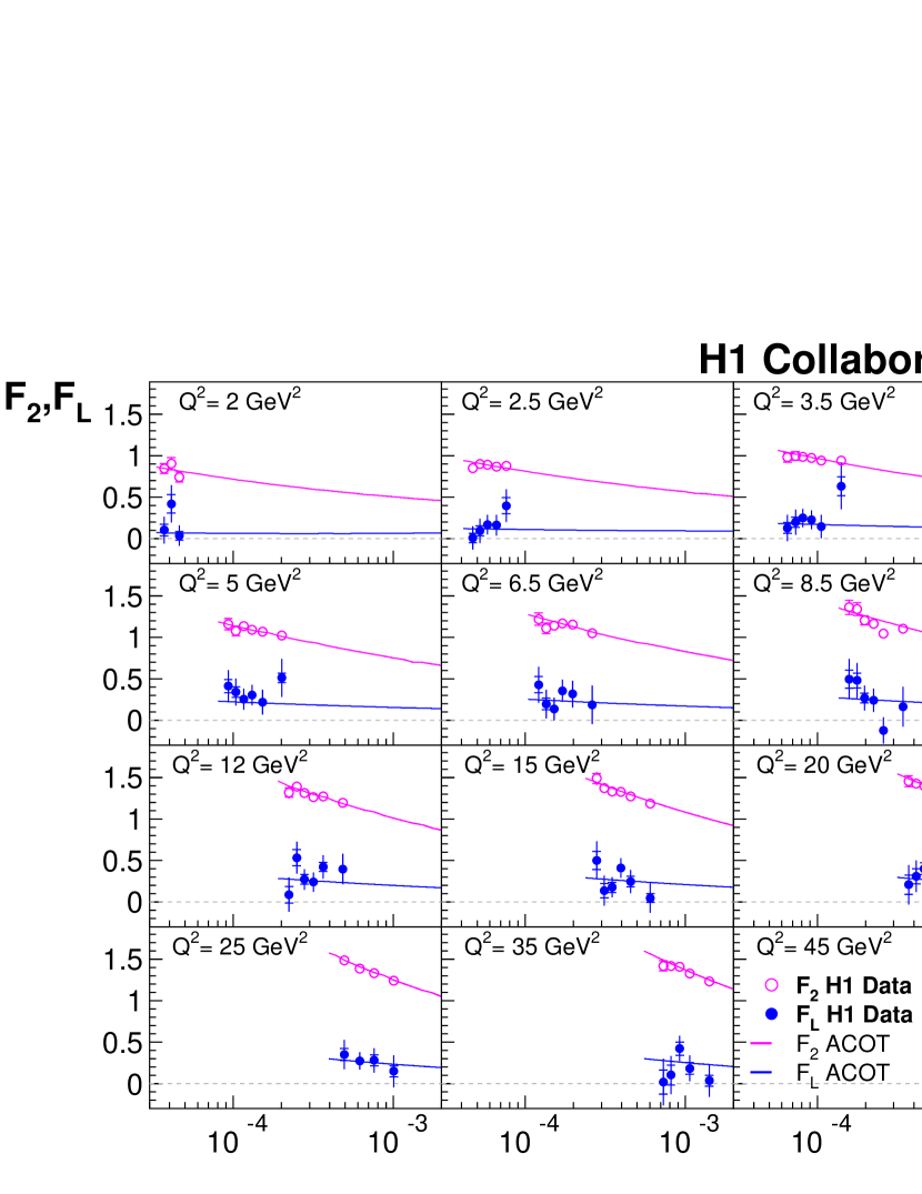
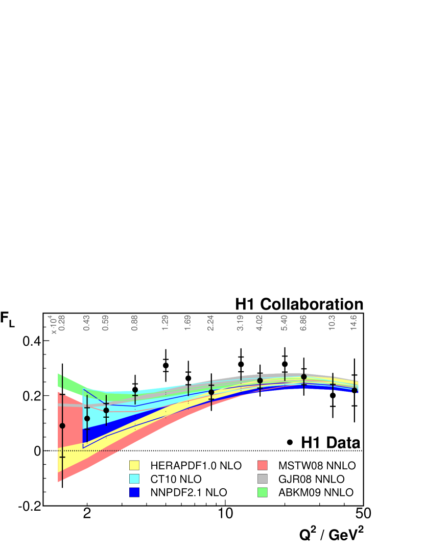
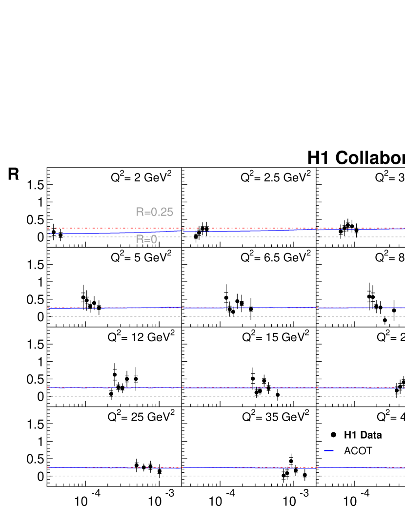

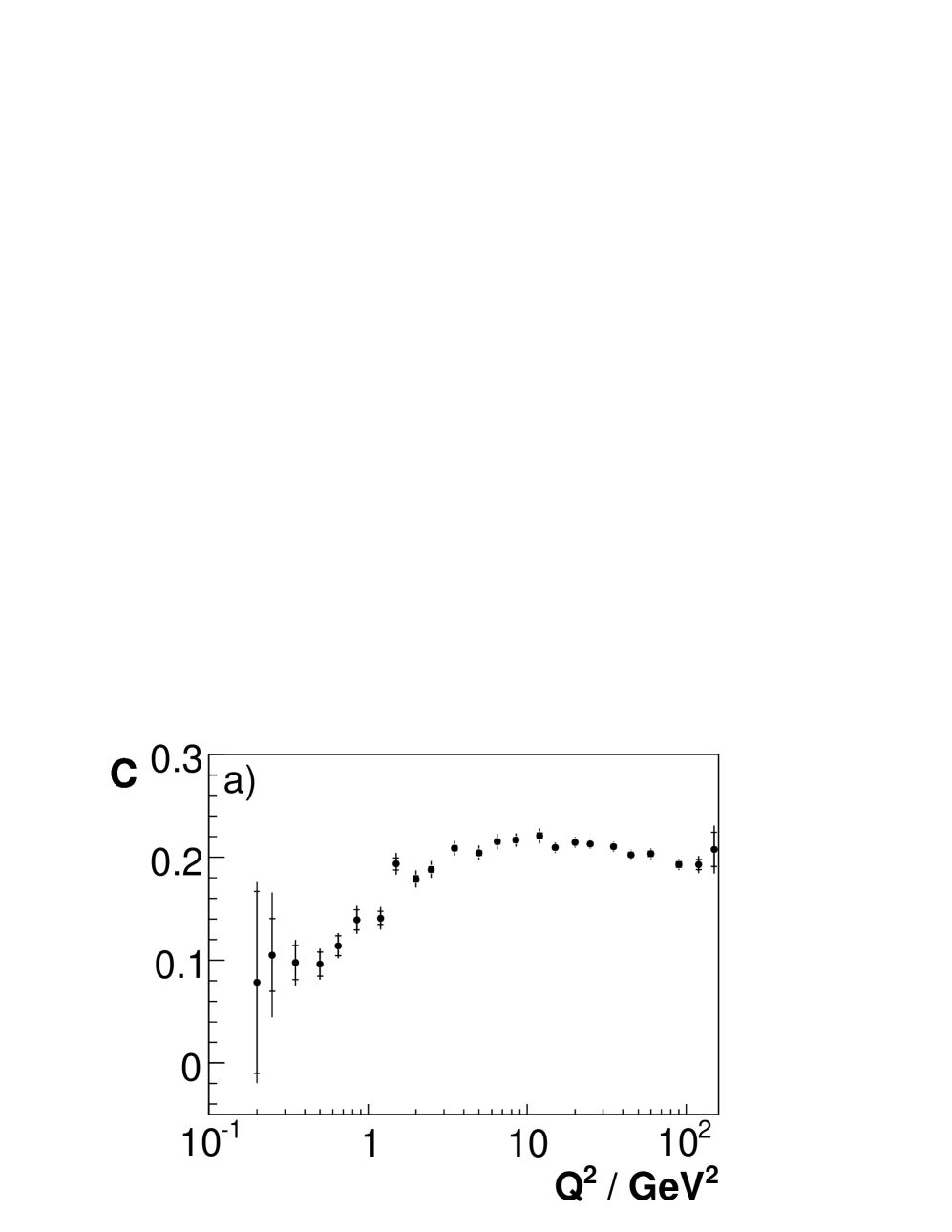
|
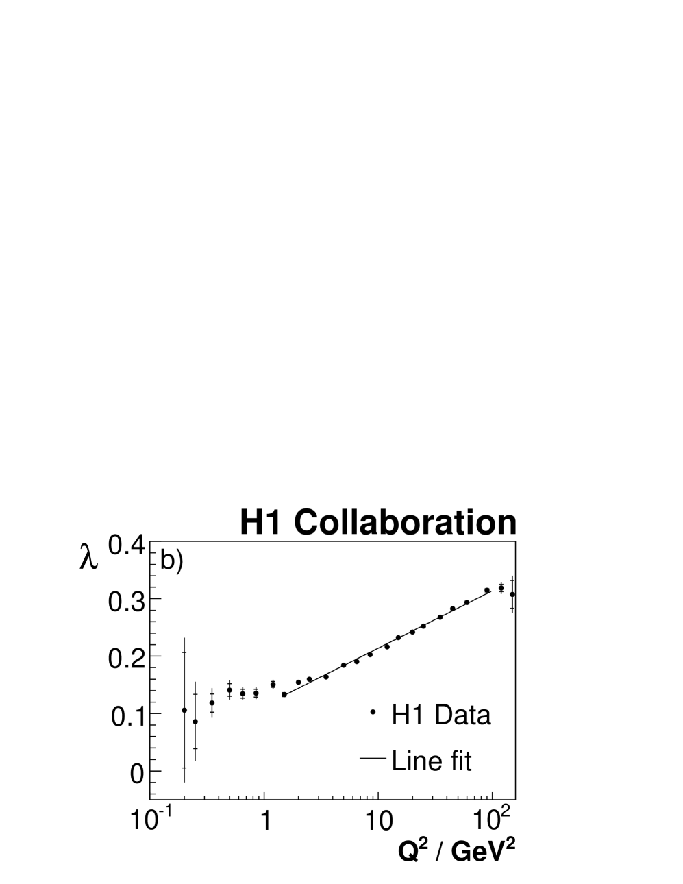
|

|
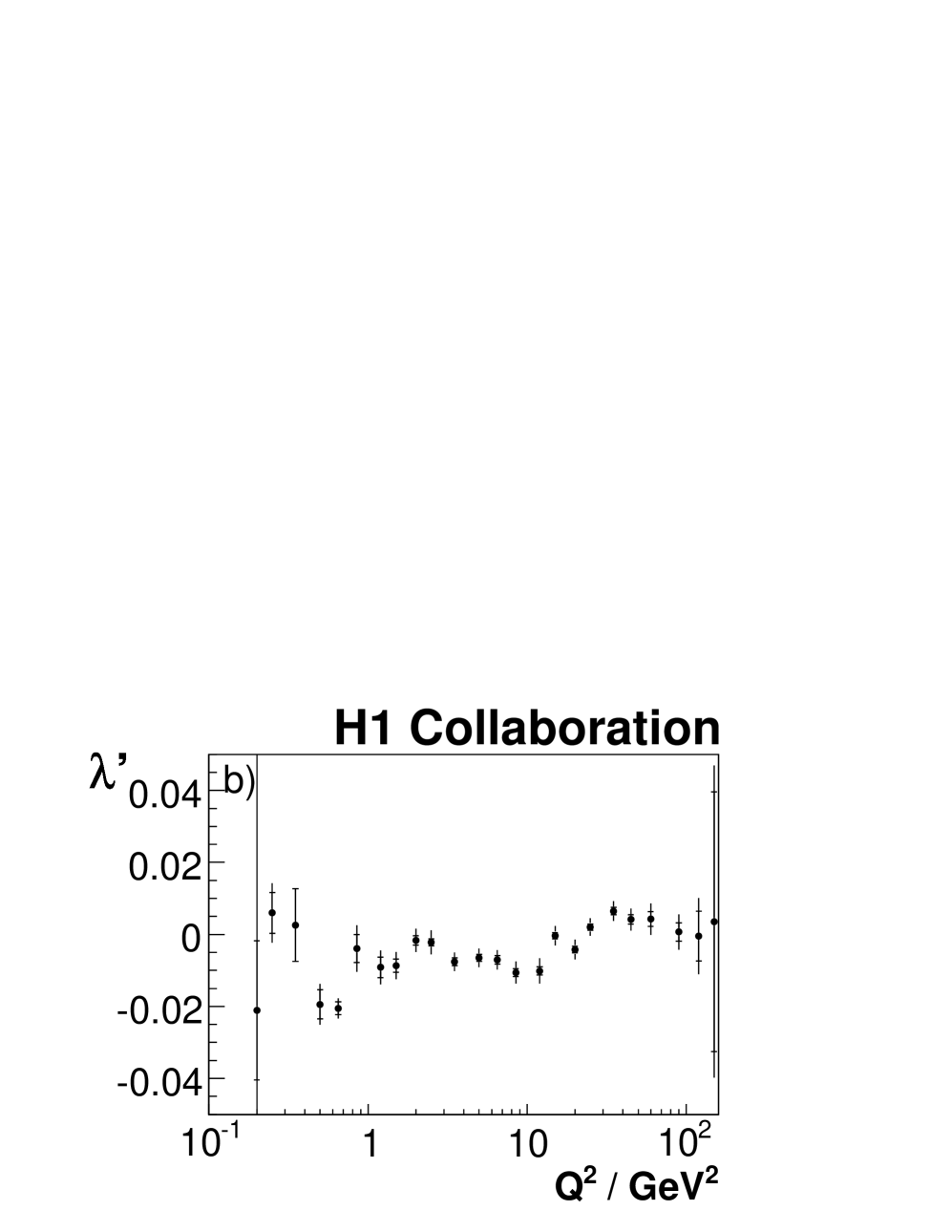
|

|
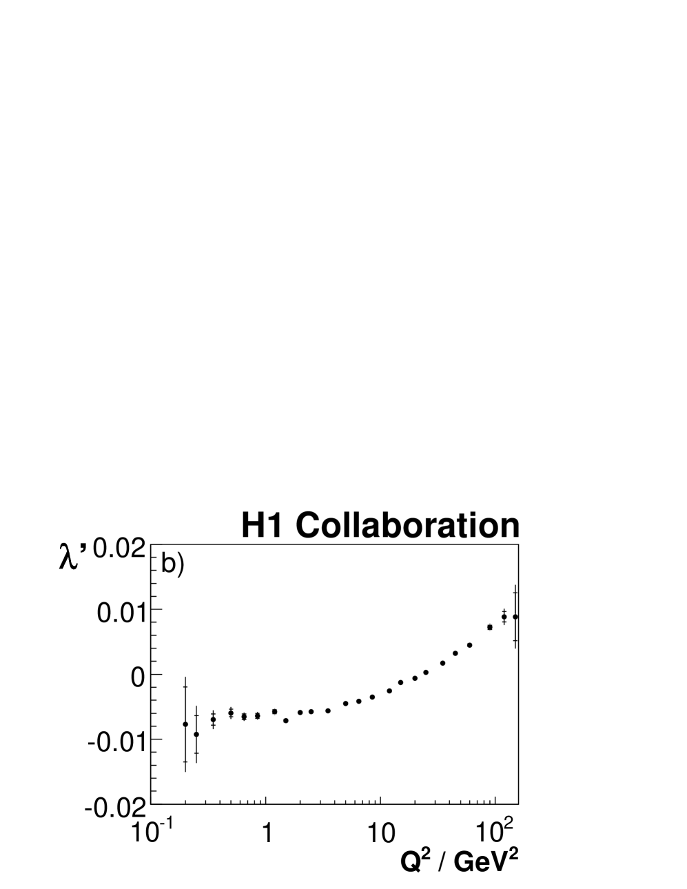
|