Linear AC Response of Diffusive SNS Junctions

Abstract

We explore the behavior of the ac admittance of superconductor-normal metal-superconductor (SNS) junctions as the phase difference of the order parameters between the superconductors is varied. We find three characteristic regimes, defined by comparing the driving frequency $\omega$ to the inelastic scattering rate $\Gamma$ and the Thouless energy $E_{T}$ of the junction (typically $\hbar\Gamma\ll E_{T}$). Only in the first regime $\omega\ll\Gamma$ the usual picture of the kinetic inductance holds. We show that the ac admittance can be used to directly access some of the characteristic quantities of the SNS junctions, in particular the phase dependent energy minigap and the typically phase dependent inelastic scattering rate. Our results partially explain the recent measurements of the linear response properties of SNS Superconducting Quantum Interference Devices (SQUIDs) and predict a number of new effects.

The frequency dependent susceptibility typically reveals information about the internal dynamics of the studied systems. In the electronic case, this susceptibility is more often measured as admittance, whose frequency dependence in semiclassical models for bulk metals is due to scattering and appears for frequencies exceeding some tens of THz Ashcroft and Mermin (1976), and in wires it is dictated by stray capacitances and geometric inductance. Understanding the frequency-dependent response is moreover of importance for high-frequency devices.

In superconductors or superconducting tunnel junctions (SIS), the admittance at low frequencies is dominated by the superconducting kinetic inductance Tinkham (1996). For SIS junctions, this Josephson inductance is related to the supercurrent $I_{S}(\varphi)$ through the junction, which depends on the superconducting phase difference $\varphi$:

$$L_{J}(\varphi)^{-1}=\frac{2e}{\hbar}\partial_{\varphi}I_{S}(\varphi)\,.$$ (1)

This relation allows characterizing the current-phase relation of Josephson junctions via measurements of their ac admittance Golubov et al. (2004). The remaining dissipative part of the admittance is due to quasiparticles, is proportional to $\exp[-|\Delta-\hbar\omega|/(k_{B}T)]$ Tucker and Feldman (1985), and is important only for the high frequencies of the order of the superconducting gap $\Delta$ or temperatures $T$ close to the critical temperature.

For other types of Josephson junctions than SIS the admittance, however, can deviate from the above simple picture. In this Letter we show how combining normal metal wires (N) and superconductors (S) into SNS weak links results into an admittance that entails characteristics of the inelastic scattering rates and the inverse diffusion times through the structure. At frequencies of the order or larger than the inelastic scattering rate $\Gamma$, the simple kinetic inductance picture has to be revised to include non-adiabatic effects associated with the dynamics of the electron distribution. The dissipative response, describing microwave absorption, is moreover finite for temperatures or frequencies exceeding the phase-dependent minigap in the spectrum of excitations inside the junction. It probes the density of states in the junction, and is related to the physics of stimulation and suppression of the supercurrent Warlaumont et al. (1979); *fuechsle2009-eom; *aslamazov1982-ssb; Virtanen et al. (2010).

Here, we study diffusive SNS junctions, whose length $L$ is longer than the superconducting coherence length $\xi_{0}=\sqrt{\hbar D/\Delta}$, where $D$ is the diffusion constant. The proximity effect induces a gap in the density of states inside the normal metal, $E_{g}(\varphi=0)=3.12E_{T}\ll{}\Delta$, where $E_{T}=\hbar D/L^{2}$ is the inverse diffusion time. The minigap depends on the phase difference approximately as $\cos(\varphi/2)$ and vanishes for $\varphi=\pi$. The coupling to the electric field is modeled by assuming an ac bias voltage, $V(t)=\delta V\sin(\omega t)$, which induces an oscillating phase difference $\varphi(t)=\varphi+\delta\phi\cos(\omega t)$ across the junction.

To find quantitative results, we describe the SNS junction dynamics with the Keldysh-Usadel equation Usadel (1970); *belzig1999-qgf, used also in Ref. Virtanen et al. (2010). In this approach, physical quantities are obtained from the Retarded, Advanced and Keldysh Green’s functions $\hat{g}^{R/A/K}(E,E^{\prime})$, which depend on two energy arguments. These functions are matrices in the Nambu (electron-hole) space, and the Keldysh (K) part can be parameterized in terms of an electron distribution function matrix $\hat{h}(E,E^{\prime})=h_{L}(E,E^{\prime})+h_{T}(E,E^{\prime})\hat{\tau}_{3}$: $\hat{g}^{K}=\hat{g}^{R}\hat{h}-\hat{h}\hat{g}^{A}$, where matrix products involve also convolutions, $(\hat{B}\hat{C})(E,E^{\prime})=\int_{-\infty}^{\infty}\frac{\mathop{\mathrm{d}E_{1}}}{2\pi}\hat{B}(E,E_{1})\hat{C}(E_{1},E^{\prime})$. In the presence of the harmonic drive, these functions can be written in a matrix representation $\hat{g}_{n,m}(E)\hat{=}\hat{g}(E+n\hbar\omega,E+m\hbar\omega)$ Cuevas et al. (2006) that reduces convolutions to matrix products.

The ac admittance is $Y(\omega)=\frac{2}{i\omega\delta\phi}I(\omega)$, for a linear-response drive $\delta\phi\ll 2\pi$. The ac current harmonic is $I(\omega)=\frac{\sigma_{N}S}{4}\int_{-\infty}^{\infty}\mathop{\mathrm{d}E}{\rm Tr}\hat{\tau}_{3}\hat{j}^{K}_{01}(E)$, where $\sigma_{N}$ and $S$ are the normal-state conductivity and the cross section of the junction, and the Keldysh current is $\hat{j}^{K}=\hat{g}^{R}\hat{\partial}_{x}\hat{g}^{K}+\hat{g}^{K}\hat{\partial}_{x}\hat{g}^{A}$. Here $x$ is the position in the junction, and $\hat{\partial}_{x}\hat{B}=\partial_{x}\hat{B}-i[A\hat{\tau}_{3},\hat{B}]$ the gauge-covariant gradient containing the vector potential $A(E,E^{\prime})=A(E)\delta(E-E^{\prime})$.

In the above approach, the admittance splits naturally into three gauge-invariant parts, $Y=Y_{\rm sc}+Y_{\rm dy}+Y_{\rm qp}$, where (hereafter, $\hbar=e=k_{B}=1$)

$$Y_{\rm sc} =\frac{\sigma_{N}S}{2i\omega\delta\phi}\int_{-\infty}^{\infty}\mathop{\mathrm{d}E}\operatorname{Tr}\{\hat{\tau}_{3}(\hat{j}_{01}^{R}h_{11}-h_{00}\hat{j}_{01}^{A})\}\,,$$ (2a)

$$Y_{\rm dy} =\frac{\sigma_{N}S}{2i\omega\delta\phi}\int_{-\infty}^{\infty}\mathop{\mathrm{d}E}\operatorname{Tr}\{\hat{\tau}_{3}(\hat{j}^{R}_{00}\hat{h}_{01}-\hat{h}_{01}\hat{j}^{A}_{11})\}\,,$$ (2b)

$$Y_{\rm qp} =\frac{\sigma_{N}S}{2i\omega\delta\phi}\int_{-\infty}^{\infty}\mathop{\mathrm{d}E}\operatorname{Tr}\Bigl{\{}(1-\hat{\tau}_{3}\hat{g}_{11}^{A}\hat{\tau}_{3}\hat{g}_{00}^{R})$$ (2c)

$$\quad\times[\hat{\tau}_{3}\partial_{x}\hat{h}_{01}-\frac{iA_{0}}{2}(h_{11}-h_{00})]\Bigr{\}}\,.$$

Here $\hat{j}^{R/A}=\hat{g}^{R/A}\hat{\partial}_{x}\hat{g}^{R/A}$ describe spectral (super)currents, $h_{00}(E)=h_{11}(E-\omega)=\tanh(E/2T)$ the equilibrium electron distribution, and $\hat{h}_{01}$ its time-dependent part. The contributions describe (a) the ac supercurrent, (b) effect of the dynamic variation of the populations of the Andreev levels, and (c) the quasiparticle current driven directly by the field. Below, we mostly work in a gauge in which the electric field is contained in the vector potential, $A(t)=A_{0}\cos(\omega t)$, $A_{0}=-\delta\phi/(2L)$. Requiring charge neutrality leads to a finite position dependent scalar potential, but our numerics indicate that this can be disregarded for $\omega\lesssim{}10E_{T}$.

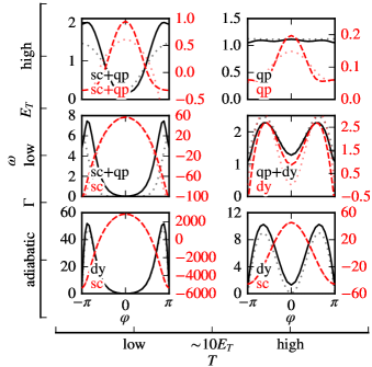
Figure 1: (Color online): Phase dependence of the admittance $Y$ in units of the normal state conductance $G_{N}$ (dissipative part: solid, reactive part: dashed), in different regimes of interest. The “low” temperature results have been calculated for $T=E_{T}$, the “high” temperature results for $T=16E_{T}$. The adiabatic frequency is $\omega=E_{T}/200\ll\Gamma=E_{T}/20$, the low $\omega=E_{T}/4\gg\Gamma$, and the high frequency is $\omega=10E_{T}$. Dotted lines show the contribution from dominant parts, $Y_{\rm sc}$ [Eqs. (1), (8)], $Y_{\rm dy}$ [Eq. (5)], $Y_{\rm qp}$ [Eqs. (7), (9)], indicated in the lower left corners. The adiabatic frequency results are obtained from analytical approximations, the others from the full numerics.

In the following, our aim is to relate the contributions (2) to quantities that can be calculated in the absence of the ac drive not . The regimes where the different contributions are relevant depend on the particular values of the phase difference, frequency and temperature. The main results are summarized in Fig. 1, which shows the phase dependence of the admittance in different regimes of frequencies and temperatures.

Low frequency: For frequencies satisfying $\Gamma\ll\omega\ll E_{g}(\varphi)$, the superconducting correlations follow the time-dependent phase difference, but the electron distribution is driven out of equilibrium. In this limit, the time-dependent supercurrent (2a) yields Eq. (1), i.e., $Y_{\rm sc}\simeq-2i\partial_{\varphi}I_{S}(\varphi)/\omega$. Since the supercurrent $I_{S}$ decays exponentially as the temperature increases, this contribution to reactance becomes unimportant at high temperatures ($T\gtrsim{}10E_{T}$), unless the frequency is very low.

The second major contribution to reactance comes from a dynamic variation of the population, as given by $Y_{\rm dy}$. For this, the time dependent component $\hat{h}_{01}\equiv{}h_{L}^{\prime}+\hat{\tau}_{3}h_{T}^{\prime}$ of the distribution function needs to be solved from a kinetic equation. Assuming again simple time dependence for the superconducting correlations, the first harmonic of the Usadel kinetic equation reads (cf. Virtanen et al. (2010))

$$D\partial_{x}\cdot({\cal D}_{L}\partial_{x}h_{L}^{\prime}-{\cal T}\partial_{x}h_{T}^{\prime}+j_{S}h_{T}^{\prime})=$$ (3a)

$$\frac{iA_{0}}{2}(j_{S}+\partial_{x}{\cal T})(h_{11}-h_{00})+i(\omega-2i\Gamma)Nh_{L}^{\prime}\,,$$

$$D\partial_{x}\cdot({\cal D}_{T}\partial_{x}h_{T}^{\prime}+{\cal T}\partial_{x}h_{L}^{\prime}+j_{S}h_{L}^{\prime})=0.$$ (3b)

Here ${\cal D}_{L/T}$ are the spectral heat/charge diffusion coefficients, ${\cal T}$ is an anomalous kinetic coefficient and $N$ is the local density of states. These quantities are related to the equilibrium Retarded Green’s function, $\hat{g}^{R}(E)=g(E)\hat{\tau}_{3}+f(E)\hat{\tau}_{\uparrow}-\tilde{f}(E)\hat{\tau}_{\downarrow}$, e.g., $j_{S}=\mathop{\mathrm{Im}}j_{E}$, $j_{E}=\frac{1}{2i}\operatorname{Tr}\hat{\tau}_{3}\hat{j}^{R}_{00}$, $N=\mathop{\mathrm{Re}}g$, and ${\cal D}_{T}=\frac{1}{2}[1+|g|^{2}+|f|^{2}/2+|\tilde{f}|^{2}/2]$.

At low frequencies, Eqs. (3) should be solved with Andreev reflection boundary conditions amounting to $h_{T}^{\prime}=0$ and $\partial_{x}\cdot h_{L}^{\prime}\hat{n}=0$ at the two NS interfaces. The resulting function $h_{T}^{\prime}$ is in the vector potential gauge finite but small, and as a first approximation we can disregard it. Moreover, gradients of $h_{L}^{\prime}$ are small due to Andreev reflection, and we get a fairly good estimate for the average $h_{L}^{\prime}$ by averaging Eqs. (3) over the normal-metal junction, defining $\langle{\cdot}\rangle=\int_{0}^{L}dx\cdot/L$. As a result, we get

$$\hat{h}_{01}\approx\langle{h_{L}^{\prime}}\rangle\approx\frac{A_{0}}{2}\frac{j_{S}(h_{11}-h_{00})}{(\omega-2i\Gamma)\langle N\rangle}.$$ (4)

Substituting this to Eq. (2b) and assuming $\omega\lesssim{}E_{T}$,

$$Y_{\rm dy} \equiv\frac{-iG_{N}}{\omega-2i\Gamma}\frac{E_{T}}{T}Q(\varphi,T)$$ (5)

$$\approx\frac{-iG_{N}}{\omega-2i\Gamma}\int_{-\infty}^{\infty}dE\frac{j_{S}^{2}}{4T\langle{N}\rangle\cosh^{2}[E/(2T)]}.$$

This is similar to a correction to the dc conductance described by Lempitskii Lempitskii (1983). Its origin can be understood as follows Chiodi et al. (2010): the current is carried by a dense spectrum $\{\epsilon_{n}(\varphi)\}$ of discrete bound states with populations $f_{n}$, $j(\varphi)=\sum_{n}(\partial_{\varphi}\epsilon_{n})f_{n}(\epsilon_{n})$. With ac bias one finds $\delta j/\delta V\propto\sum_{n}\partial_{\varphi}^{2}\epsilon_{n}f_{n}/i\omega+\sum_{n}(\partial_{\varphi}\epsilon_{n})^{2}\partial_{\epsilon}f_{n}/i\omega$, where the first term is equivalent to $Y_{\rm sc}$ and the second one to $Y_{\rm dy}$, as $j_{S}\sim{}\sum_{n}\delta(E-\epsilon_{n})\partial_{\varphi}\epsilon_{n}\sim{}N\partial_{\varphi}\epsilon$.

The dynamic contribution is purely dissipative and constant for $\omega\ll\Gamma$, contains both reactive and dissipative components for $\omega\approx\Gamma$, and becomes purely reactive and decays for $\omega\gg\Gamma$, as visible in Fig. 1. In general, $\Gamma$ also depends on the phase difference Heikkilä and Giazotto (2009), so that the phase-dependent response at frequencies of the order of the inelastic scattering rate may be quite complicated. On the other hand, Eq. (5) offers a way to probe such phase-dependent scattering rates via an admittance measurement.

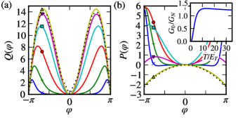
Figure 2: (Color online): (a) Function $Q(\varphi,T)$ (see Eq. (5)) describing the phase-dependent dynamic contribution to the reactive response and (b) function $P(\varphi,T)$ (Eq. (7)) describing the phase dependence of the dissipative part of the admittance at low frequencies. From top to bottom in (a) and marked with symbols in (b): $T/E_{T}=16(\vartriangle),8(\triangledown),4(\square),2(\circ),1(+),0.5(\times)$. The dotted lines represent the analytic high-temperature approximations to which $Q$ and $P$ tend for $T\gg E_{T}$. The inset of (b) shows the temperature dependence of $G_{0}(T)$.

The function $Q(\varphi,T)$ is shown in Fig. 2(a) for different temperatures. At $T\gg E_{T}$ the response can be fitted with the function $Q(\varphi)\approx 8.9\bigl{(}|\operatorname{saw}(\varphi)|-0.32\sin^{2}(\varphi/2)\bigr{)}|\sin(\varphi)|$ where $\operatorname{saw}(\varphi)=(\varphi+\pi\mod 2\pi)-\pi$. At low temperatures, $Q(\varphi,T)$ is suppressed for phases at which $T<E_{g}(\varphi)$. Note that $Q$ is positive definite, has almost a double periodicity compared to the kinetic inductance term, and has a minimum around $\varphi=0$, where the kinetic inductance is at maximum.

The dissipative part of the impedance originates from two additional sources: the quasiparticle part $Y_{\rm qp}$, and, importantly at low temperatures, a part of the AC supercurrent oscillating in phase with the voltage. The quasiparticle contribution is easiest to derive in a gauge where the vector potential vanishes. Then, $h_{T}^{\prime}$ in Eqs. (3) has the boundary conditions $h_{T}^{\prime}(x=\pm{}L/2)=\pm\frac{i\delta\phi}{4}(h_{11}-h_{00})$, and solving Eq. (3) assuming $h_{L}^{\prime}\approx 0$ yields

$$Y_{\rm qp}+\mathop{\mathrm{Re}}Y_{\rm sc} \simeq G_{N}\int_{-\infty}^{\infty}\mathop{\mathrm{d}E}\frac{K_{0}(E)}{4T\cosh^{2}[E/(2T)]}\,,$$ (6)

$$\equiv G_{0}(T)+\frac{G_{N}E_{T}}{T}P(\varphi,T),$$ (7)

where we assumed $\omega\lesssim{}E_{T}$, and defined $G_{0}(T)$ as the $\varphi=0$ value [$P(0,T)=0$]. The kernel is $K_{0}\approx\langle{{\cal D}_{T}^{-1}}\rangle^{-1}-\mathop{\mathrm{Re}}\partial_{\varphi}j_{E}\sim{}\langle{N^{2}+\frac{1}{4}|f+\tilde{f}^{*}|^{2}}\rangle$ . It describes the spectrum of excitations in the junction available for receiving energy — this has a minigap $E_{g}(\varphi)$, so that for $\omega,T<E_{g}(\varphi)$ all dissipation vanishes. Note that the appearance of the minigap is related to the presence of the AC supercurrent contribution: $Y_{\rm qp}\geq{}G_{N}$ and is similar to the usual proximity-enhanced conductance.

The functions $P(\varphi,T)$ and $G_{0}(T)$ are shown in Fig. 2(b). At low temperatures, the temperature and phase dependence shows a clear signature of the presence of a minigap in the density of states; note that this also applies to the $Y_{\rm dy}$ contribution. The dissipation is concentrated at phase differences close to $\pi$ where the minigap is small. In the high-temperature limit, the dissipative term consists of a phase independent contribution $G_{0}(T)$ and the phase-dependent part has a simple phase and temperature dependence, $-0.23\operatorname{saw}(\varphi)^{2}G_{N}E_{T}/T$.

High frequency: When the frequency becomes of the order of the Thouless energy $E_{T}$, the above semi-adiabatic expressions break down as the spectral quantities become frequency dependent. We can however construct approximations also in this limit (for full expressions, see Appendix). The supercurrent contribution is fairly approximated by

$$\begin{split}Y_{\rm sc}&\approx\frac{\sigma_{N}S}{4\omega}\int_{-\infty}^{\infty}\mathop{\mathrm{d}E}\bigg{\{}\partial_{\varphi}[j_{E}(E)+j_{E}(E+\omega)]^{*}h_{00}(E)\\ &\qquad-\partial_{\varphi}[j_{E}(E)+j_{E}(E+\omega)]h_{11}(E)\bigg{\}},\end{split}$$ (8)

and the quasiparticle part of the impedance by

$$Y_{\rm qp} \simeq G_{N}\int_{-\infty}^{\infty}dEK(E,\omega)\frac{h_{11}(E)-h_{00}(E)}{2\omega}\,,$$ (9)

$$K(E,\omega)=\frac{1}{2}\Bigl{\langle}\bigl{[}1+g(E)g(E+\omega)^{*}$$ (10)

$$\;+\frac{1}{2}f(E)f(E+\omega)^{*}+\frac{1}{2}\tilde{f}(E)\tilde{f}(E+\omega)^{*}\bigr{]}^{-1}\Bigr{\rangle}^{-1}\,.$$

The dynamic contribution $Y_{\rm dy}$ can be neglected for $\omega\gg{}E_{T}$. The above is compared to full numerical solutions in the top panels in Fig. 1.

At high temperatures, $Y_{\rm sc}$ is exponentially suppressed even for high frequencies, similarly as the equilibrium supercurrent. Consequently, $Y_{\rm qp}$ dominates for $\omega,T\gg{}E_{T}$ (see Fig. 1). At low temperatures, both the supercurrent and quasiparticle contributions are important.

The amplitude of the phase dependence in the admittance is illustrated in Fig. 3, up to high frequencies. As the frequency increases, the proximity-induced phase dependence in the reactive and the dissipative components decays, as the admittance approaches the constant normal-state value, $Y(\omega,\varphi)\to{}G_{N}$. Similarly, the phase dependence vanishes as the temperature increases. At low frequencies, on the other hand, the reactive component diverges due to the Josephson inductance, and the dissipative component is dominated by $Y_{\rm dy}$.

Figure 3: (Color online): Amplitude $\delta{}Y=\max_{\varphi}[\mathop{\mathrm{Re}}/\mathop{\mathrm{Im}}]Y(\varphi)-\min_{\varphi}[\mathop{\mathrm{Re}}/\mathop{\mathrm{Im}}]Y(\varphi)$ of the phase-dependence in the nonadiabatic dissipative (Re) and reactive (Im) admittance of a long SNS junction, obtained by solving the time-dependent Usadel equations numerically. The lines correspond to temperatures $T/E_{T}=0.5,1,2,4,8,16$ (top to bottom) and were calculated with $\Gamma=0.05E_{T}$.

In a recent experiment probing directly the ac admittance of SNS junctions Chiodi et al. (2010), it was found that at frequencies $\Gamma\ll\omega\ll{}E_{T}$ (semi-adiabatic limit), the reactive response follows closely our prediction consisting of the sum of the Josephson inductance and the dynamical correction (5). However, both the dissipative contribution and the dependence at high frequencies $\omega\gtrsim E_{T}$ are different: in Chiodi et al. (2010), the dissipative contribution is directly related to the reactive contribution, and moreover the amplitude of phase oscillations in susceptibility $\delta\chi=i\omega\delta Y$ decays as frequency increases. The characteristic frequency scale for this was found to be temperature independent and of the order of the Thouless energy. In contrast, in this frequency range our Usadel model predicts $\delta\chi\sim\text{const.}$ — however, it is for example possible that the simple relaxation time approximation does not include all interaction mechanisms playing a role in the experiment.

Finally, we remark that our work amounts essentially to deriving the parameters for the Resistively Shunted Junction (RSJ) model of SNS junctions Tinkham (1996): there, the Josephson inductance resulting from the supercurrent term should be modified to include the nonadiabatic correction, Eq. (5), and the shunt resistor describing the dissipation in the junction should be replaced by the dissipative terms presented in Eqs. (5,7).

In conclusion, we have described the frequency-dependent admittance of diffusive superconductor-normal metal-superconductor junctions and shown how the simple adiabatic Josephson inductance picture is modified once the frequency is increased. Besides studying the dynamics of the system, the detailed frequency dependence can be used to study directly the inelastic scattering rates. Our results are also relevant for devices utilizing high-frequency properties of SNS junctions, such as those used in metrology and radiation detection.

We thank H. Bouchiat, S. Gueron, K. Tikhonov, and M. Feigelman for discussions that in part motivated this work, and CSC (Espoo) for computer resources. This work was supported by the Academy of Finland, the ERC (Grant No. 240362-Heattronics), the Spanish MICINN (Contract No. FIS2008-04209), and the Emmy-Noether program of the DFG.

Appendix A On approximations

Although one cannot solve the time-dependent linear-response Usadel equations analytically in closed form, the admittance can be obtained with quantitative accuracy if the solution at equilibrium is known. The approximation procedure is outlined in the main text. Below, we show intermediate results before taking the $\omega\to 0$ limit, and demonstrate that the results agree with the full numerical approach which solves the ac Usadel equation exactly (see the Supplementary information of Ref. Virtanen et al., 2010 for details of the numerics).

Following the procedure outlined in the main text, the following approximations can be derived:

$$Y =\sigma S\int_{-\infty}^{\infty}dE\>\tilde{Y}(E)=\sigma S\int_{-\infty}^{\infty}dE\>[\tilde{Y}_{\rm sc}(E)+\tilde{Y}_{\rm dy}(E)+\tilde{Y}_{\rm qp}(E)]\,,$$ (11a)

$$\tilde{Y}_{\rm sc}(E) \simeq\frac{-1}{2\omega}\Bigl{(}\frac{\partial_{\phi}[j_{E}(E)+j_{E}(E+\omega)]}{2}h(E+\omega)-\frac{\partial_{\phi}[j_{E}(E)+j_{E}(E+\omega)]^{*}}{2}h(E)\Bigr{)}\,,$$ (11b)

$$\tilde{Y}_{\rm dy}(E) \simeq\frac{1}{8\omega}\frac{i}{\omega-2i\Gamma}\frac{(j_{E}(E)-j_{E}(E+\omega)^{*})^{2}}{\frac{1}{2}\langle{}g(E)+g(E+\omega)^{*}\rangle}(h(E+\omega)-h(E))\,,$$ (11c)

$$\tilde{Y}_{\rm qp}(E) \simeq\frac{1}{4\omega}\bigl{\langle}[1+g(E)g(E+\omega)^{*}+\frac{1}{2}f(E)f(E+\omega)^{*}+\frac{1}{2}\tilde{f}(E)\tilde{f}(E+\omega)^{*}]^{-1}\bigr{\rangle}^{-1}(h(E+\omega)-h(E))\,.$$ (11d)

Above, $h(E)=\tanh[E/(2T)]$, and the energy-dependent quantities $j_{E}(E)=\frac{-i}{2}\operatorname{Tr}[\hat{\tau}_{3}\hat{g}^{R}\nabla\hat{g}^{R}]$ and $\hat{g}^{R}(E)=g(E)\hat{\tau}_{3}+f(E)\frac{\hat{\tau}_{1}+i\hat{\tau}_{2}}{2}-\tilde{f}(E)\frac{\hat{\tau}_{1}-i\hat{\tau}_{2}}{2}$ are obtained from the equilibrium Usadel equations Belzig et al. (1999); Usadel (1970), which are much faster to solve than the full ac equations.

Figures 4, 5, and 6 illustrate that the above approximations reproduce all qualitative features visible in the fully numerical solution, and are quantitatively accurate in a large part of the parameter regime we are interested in. In particular, the deviations between the two approaches are miniscule for frequencies lower than $E_{T}$. At large frequencies there are clear quantitative differences, but the qualitative phase and frequency dependence is the same, and the resulting admittances are of the same order of magnitude. This demonstrates that to a fair accuracy the ac admittance can be well described by using Eqs. (11) and standard solvers for the equilibrium Usadel equation. Besides that, Eq. (11) provides a possibility for making analytical estimates for the admittance contributions.

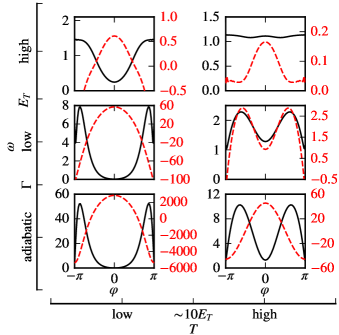
Figure 4: Left: Fig. 1 in the main text. Right: Fig. 1 with all data computed from Eqs. (11).

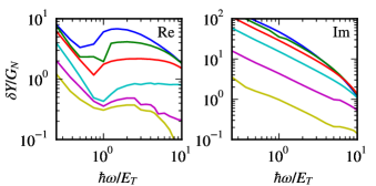
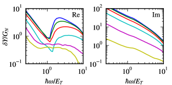
Figure 5: Left: Fig. 3 in the main text. Right: Fig. 3 with all data computed from Eqs. (11).

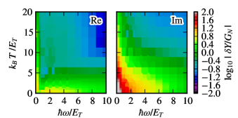
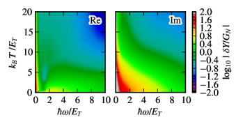
Figure 6: As Fig. 3 in the main text, but expressed as a color plot. Left: numerically computed admittance oscillations. Right: admittance oscillations from Eqs. (11).

References

Ashcroft and Mermin (1976)N. Ashcroft and N. Mermin, Solid State Physics (Saunders College, Philadelphia, 1976).
Tinkham (1996)M. Tinkham, Introduction to
Superconductivity, 2nd ed. (McGraw-Hill, New York, 1996).
Note (1)The latter approximation is the one used in Virtanen et al. (2010) and captures the minigap correctly, whereas the former
gives a better approximation to the integral, but is inaccurate at energies
.