Experimental and theoretical lifetimes and transition probabilities in Sb I

Abstract

We present experimental atomic lifetimes for 12 levels in Sb I, out of which seven are reported for the first time. The levels belong to the 5p²(³P)6s ²P, ⁴P and 5p²(³P)5d ⁴P, ⁴F and ²F terms. The lifetimes were measured using time-resolved laser-induced fluorescence. In addition, we report new calculations of transition probabilities in Sb I using a Multiconfigurational Dirac-Hartree-Fock method. The physical model being tested through comparisons between theoretical and experimental lifetimes for 5d and 6s levels. The lifetimes of the 5d ⁴F_3/2,5/2,7/2 levels (19.5, 7.8 and 54 ns, respectively) depend strongly on the $J$-value. This is explained by different degrees of level mixing for the different levels in the ⁴F term.

I Introduction

As many other spectra, Sb I was first investigated by Meggers & Humphreys MH42 . Since then the analysis has been extended and revised by Mazzoni & Joshi MJ79 , Joshi et al. JSV84 , Zaidi et al. ZMB84 , Beigang & Wynne BW86 and Voss et al. VWBW86 . The most recent and complete work is that of Hassini et al. HARVW88 who reported 138 levels derived from 617 spectral lines measured in the range 2536 to 24786 cm^-1, using Fourier transform spectroscopy. Of the reported levels 32 were previously unknown and several previous levels assignments were revised. Furthermore, Hassini et al. HARVW88 reported hyperfine splitting constants for more than 75 % of the levels.

Belin et al. BGHR74 measured radiative lifetimes of the two levels (³P)6s ⁴P_3/2 and ⁴P_5/2 using the Hanle-effect method. Andersen et al. AWS74 measured six levels ((³P)6s ⁴P_1/2,3/2,5/2, ²P_3/2, and (¹D)6s ²D_3/2,5/2) using the beam-foil method. Furthermore, 14 lifetimes measured with beam foil, level-crossing and multichannel delayed-coincidence detection were reported by Osherovich & Tezikov OT77 and Tezikov T78 for levels in the 6s, 7s, and 8s configurations.

Transition probabilities and lifetimes in neutral antimony are still very scarce. In astrophysics, this explains e.g. why the most recent compilation of solar abundances GASS does not provide any result for the photospheric abundance of this element while the meteoritic result is well establised. This is partly due to the fact that the lines identified as Sb I in the solar spectrum MMH are severely blended but also to the fact that reliable oscillator strengths are still lacking for these transitions.

In the present paper, we report experimental lifetimes for 12 Sb I levels measured with time-resolved laser-induced fluorescence (TR-LIF) spectroscopy. Seven of the levels are reported for the first time. In addition, we report calculated lifetimes and transition probabilities using a Multiconfigurational Dirac-Hartree-Fock (MCDHF) method. The accuracy of the calculations is assessed through the good agreement observed between theoretical and available experimental lifetimes and branching fractions.

II The Sb I term system

The spectrum of neutral antimony (Sb I) is homologous with that of N I, with the lowest configuration $n$s²$n$p³ (in Sb I, $n=5$). Due to the Pauli exclusion principle, this configuration contains only three terms: ⁴S^∘, ²D^∘ and ²P^∘, out of which ⁴S^∘ is the ground state. The system, with one excited p-electron, can be written as $5$s²$5$p² $nl$, and has the three parent terms, ³P^∘, ¹D^∘ and ¹S^∘, which are the lowest terms in Sb II. The lowest even configuration is (³P)6s containing a ⁴P and a ²P term. There are no experimentally known levels belonging to the doubly excited system 5s²5p $nln^{\prime}l^{\prime}$, or to the system where one or both of the 5s electrons are excited.

Figure 1 shows a partial energy level diagram of Sb I, including the levels measured in this work. Both terms in the (³P)6s configuration are plotted in Fig. 1, but only three of the six terms (⁴P, ⁴D, ⁴F, ²P, ²D and ²F) in the (³P)5d configuration.

Figure 1: Partial energy level diagram of Sb I including the levels measured in this work. The lines connecting the levels show the excitation routes used for the LIF experiment.

Figure 2: Extracted lifetime of the 6s ⁴P_5/2 level as a function of the delay between the ablation and the excitation laser pulses, illustrating the severe saturation effect that occurs because the level is pumped from the ground state.

Figure 3: Semi-logarithmic plot of the decay of the different fine structure levels in the 5d ⁴F term, illustrating the strong $J$-dependence found in the lifetimes. The signal registered before and during the excitation laser pulse is omitted, and the data is not background corrected. The decay of the metastable ⁴F_9/2 level could not be measured.

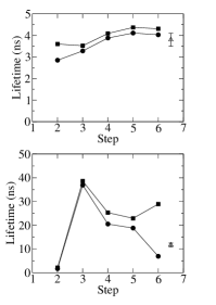
Figure 4: Examples of convergence monitoring in which the MCDHF lifetime (in ns) is plotted as function of the computation step (see the text). Filled circles and the filled squares represent the Babushkin and the Coulomb gauge values, respectively. Upper panel: $\rm(^{3}P)5d~{}^{2}F_{7/2}$ level, our TR-LIF measurement is shown with its error bar as an open triangle. Lower panel: $\rm(^{3}P)5d~{}^{4}D_{1/2}$ level, the measurement of Osherovich & Tezikov OT77 is shown with its error bar as an open triangle.

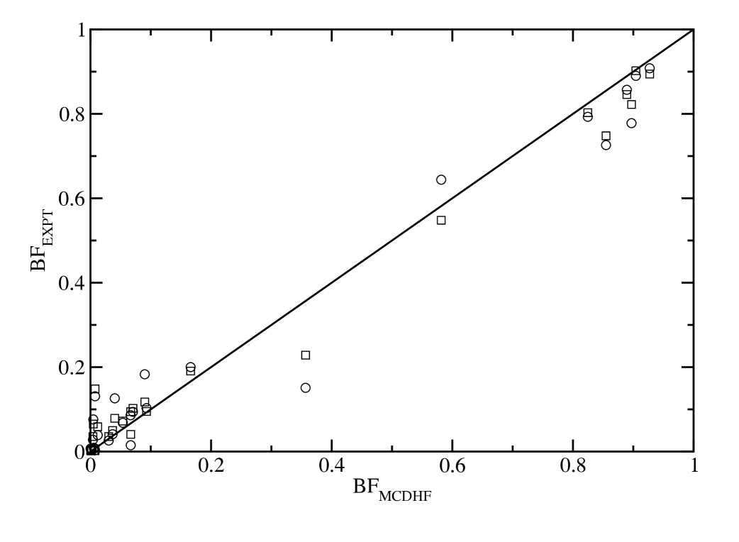
Figure 5: Comparison between corrected MCDHF (in the Babushkin gauge) and experimental branching fractions ($BF$). Circles: Guern & Lotrian GL . Squares: Gonzalez et al. GOC . A straight line of equality is drawn.

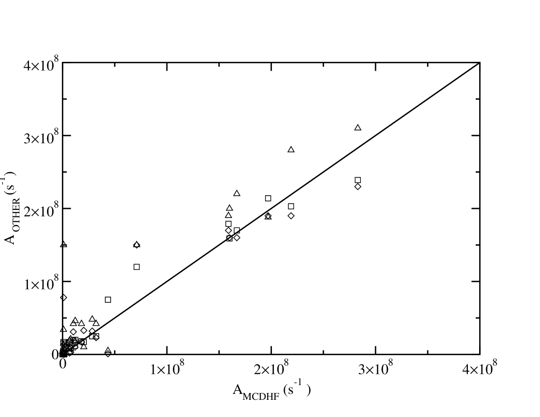
Figure 6: Comparison between corrected MCDHF transition probabilities (in the Babushkin gauge) and theoretical values taken from the literature. Squares: HF+MC calculation GOC . Diamonds: MC+CI calculation (in the Babushkin gauge) BM . Triangles: relativistic OHFS calculation (in the length gauge) HOL . A straight line of equality is drawn.

III Lifetime measurements

The lifetimes were measured at the Lund High Power Laser Facility, Sweden, using the TR-LIF technique. For a detailed description of the instrumentation, see BFHLPW88 , XJZDSBQ03 and XPSBMPB04 .

A laser-produced plasma was created by focusing a 10 Hz frequency doubled Nd:YAG laser onto a rotating antimony target, placed inside a vacuum chamber with a pressure of $\sim 10^{-5}$ millibar. The produced plasma contained free antimony atoms in the ground and excited states. Antimony atoms in low lying levels were selectively excited to the states under investigation and the subsequent fluorescence light was monitored as a function of time.

The atoms were excited by crossing the ablation plasma 1 cm above the target with a (typically) 1.2 ns duration pulse from a dye laser pumped by a Nd:YAG laser. The pump laser pulses were shortened using stimulated Brillouin scattering. The desired wavelengths were obtained using a DCM dye, making the laser tunable between 600 and 660 nm. BBO and KDP doubling and tripling crystals were used to reach shorter wavelength. In addition, a hydrogen Raman shifter was used to change the frequency of the light by one or more Stokes or anti-Stokes shifts. The delay between the ablation and excitation pulses was tuned to make the plasma contain only slow atoms, decreasing flight-in and flight-out effects and collisional quenching. For all 6s-levels, except ²P_3/2, the pumping laser was tuned to excite from the ground ⁴S${}^{\circ}_{3/2}$ state (Fig. 1). Because of the strong reabsorption from the ground state, saturation effects turned out to be very important resulting in far too long experimental 6s lifetimes unless there was a long delay between the ablation and excitation laser pulses, leading to a plasma of sufficiently low-density. This effect is clearly illustrated in Fig. 2. In the case of 6s ²P_3/2 level, the excitation was from the 5p^3 2P${}^{\circ}_{3/2}$ level where no such effect could be seen and a typical delay of around 5 $\mu$s was used.

The fluorescence signal was focused on a 1/8 m monochromator, equipped with a PMT microchannel plate (Hamamatsu R1564) to detect the fluorescence signal. The laser pulse was detected separately with a photodiode. The fluorescence signal and the temporal shape of the laser pulse were recorded simultaneously with a transient digitizer and averaged over 1000 laser pulses.

The short lifetimes were extracted by least square fitting of the fluorescence signal with a single exponential convoluted with the shape of the laser pulse, and a background function. Long lifetimes ($\tau>10$ ns) were extracted by fitting a single exponential and a background function to the fluorescence signal after the excitation pulse had died off completely. When possible we used different channels for excitation and detection of the fluorescence and more than one pump and/or detection channel as seen in Table I. However, in some cases only one channel was accessible, and the pumping and detection had to be done in the same channel.

In Table I we report the excitation and detection (fluorescence) wavelengths, and the scheme used to excite the levels. The reported lifetimes in Table II are averages of 10 to 20 lifetime curves and the uncertainties quoted include both statistical and systematic uncertainties. For comparison we give values from previous experiments found in the literature. The fourth column gives our theoretical lifetimes calculated with the MCDHF model and corrected by the experimental transition energies of Hassini et al. HARVW88 .

IV Calculations in Sb I

In order to calculate the lifetimes of the 6s and 5d levels measured in this work, we have used the MCDHF method implemented in the GRASP2K computer package JFG . In this method, the atomic state functions (ASF), $\Psi(\gamma JM_{J})$, are expanded in linear combinations of configuration state functions (CSF), $\Phi(\alpha_{i}JM_{J})$, according to

$$\Psi(\gamma JM_{J})=~{}\sum_{i}c_{i}\Phi(\alpha_{i}JM_{J}).$$ (1)

The CSFs are in turn linear combinations of Slater determinants constructed from monoelectronic spin-orbitals of the form:

$$\varphi_{n\kappa m}(r,\theta,\phi)=~{}\frac{1}{r}\begin{pmatrix}P_{n\kappa}(r)\chi_{\kappa m}(\theta,\phi)\\ iQ_{n\kappa}(r)\chi_{-\kappa m}(\theta,\phi)\end{pmatrix}$$ (2)

where $P_{n\kappa}(r)$ and $Q_{n\kappa}(r)$ are, respectively, the large and the small component of the radial wave functions, and the angular functions $\chi_{\kappa m}(\theta,\phi)$ are the spinor spherical harmonics GRA . The $\alpha_{i}$ represent all the one-electron and intermediate quantum numbers needed to completely define the CSF. $\gamma$ is usually chosen as the $\alpha_{i}$ corresponding to the CSF with the largest weight $\arrowvert c_{i}\arrowvert^{2}$. The quantum number $\kappa$ is given by

$$\kappa=~{}\pm(j+\frac{1}{2})$$ (3)

where $j$ is the electron total angular momentum. The sign before the parenthesis in Eq. (3) corresponds to the coupling relation between the electron orbital momentum, $\ell$, and its spin, i.e.

$$\ell=~{}j\pm\frac{1}{2}.$$ (4)

The radial functions $P_{n\kappa}(r)$ and $Q_{n\kappa}(r)$ are numerically represented on a logarithmic grid and are required to be orthonormal within each $\kappa$ symmetry. In the MCDHF variational procedure, the radial functions and the expansion coefficients $c_{i}$ are optimized to self-consistency.

We considered the active space (AS) method for building the MCDHF multiconfiguration expansions. The latter are produced by exciting the electrons from the reference configurations to a given set of orbitals. The rules adopted for generating the configuration space differ according to the correlation model being used. Within a given correlation model, the AS of orbitals spanning the configuration space is increased to monitor the convergence of the total energies and the transition probabilities.

The MCDHF calculations have been carried out in 6 steps.

In the first step, the core orbitals, i.e. 1s to 4d, together with the 5s and 5p orbitals, have been optimized. The 6 CSF belonging to the ground configuration 5s²5p³ were retained in the configuration space. The energy functional was built within the framework of the Average Level (AL) option GRA .

The second step consisted in increasing the configuration space by considering all the 62 CSF belonging to the following configurations: 5s²5p³+5s²5p²{6s,6p,5d}¹. The 6s, 6p and 5d orbitals have been optimized keeping the others fixed to their values of the first step. The AL option was chosen to build the energy functional.

In the third step, the configuration space has been extended to 13640 CSF by considering the single and double virtual electron excitations to the active orbital set {5s,5p,5d,6s,6p,6d} from the multireference configurations 5s²5p³+5s²5p²{6s,6p,5d}¹. Only the 6d orbital has been optimized fixing all the others to the values of the preceeding step using an energy functional built from the lowest 62 ASF within the framework of the Extended Optimal Level (EOL) option GRA . One can notice that, from this step of the computation and on, core-valence and core-core correlations are also considered through the single and double excitations of the 5s core electrons, respectively.

The last three steps consisted in extending further the configuration space by adding to the active set of the preceeding steps the following orbitals : 7s, 7p and 7d in the fourth step giving rise to 41 603 CSF; 8s, 8p and 8d in the fifth step generating 85 130 CSF; and finally, 4f in the last step with 118 912 CSF generated. In these steps, only the added orbitals have been optimized, the others being fixed using the same energy functional as in the third step; also, single and double virtual electron excitations from the same multireference configurations as in the third step have been used to generate the configuration spaces. Further orbital additions to the active set as well as further opening of the core to include more core-valence and core-core correlations have been prevented by the memory limitations of our computer.

Two examples of convergence monitoring are shown in Fig. 4. The MCDHF lifetimes of the $\rm(^{3}P)5d~{}^{2}F_{7/2}$ and $\rm(^{3}P)5d~{}^{4}D_{1/2}$ levels as computed in the Babushkin and the Coulomb gauges are plotted as function of the computation step. The values of the last step can be compared to our TR-LIF measurement for the $\rm(^{3}P)5d~{}^{2}F_{7/2}$ level and to the delayed coincidence measurement of Osherovich & Tezikov OT77 for the $\rm(^{3}P)5d~{}^{4}D_{1/2}$ level. As one can see, in the case of $\rm(^{3}P)5d~{}^{2}F_{7/2}$, the calculated lifetime converges in both gauges to the experimental value whereas it clearly diverges in the case of $\rm(^{3}P)5d~{}^{4}D_{1/2}$. The divergence of the MCDHF lifetime was also noticed for the $\rm(^{3}P)5d~{}^{4}D_{5/2},^{4}P_{1/2}$ levels not shown here. These three 5d states are probably not properly represented due to missing correlations, e.g. with $n$f and $n$g ($n\geq 5$) orbitals.

In Table 2, we report the MCDHF energies of the levels for which lifetime measurements are available. The corresponding MCDHF lifetimes and transition probabilities of main decay branches (presented in Table 3) have been corrected by the experimental transition energies of Hassini et al. HARVW88 as already stated in the previous section. Values affected by convergence problems are marked with an asterisk.

All the computed values reported here are without Breit and QED interactions. Rough estimates of the importance of these interactions on the lifetimes have been established in the second step of the computation; the lifetimes changed by less than 5%.

V Discussion

The 12 measured levels in Sb I are reported in Table II. Among them, 7 levels had not been previously considered.

Comparing the TR-LIF lifetimes from this work with values in the literature, we agree within the uncertainties with Belin et al. BGHR74 and Andersen et al. AWS74 . However, there is a clear discrepancy when comparing to Osherovich & Tezikov OT77 .

It is interesting to note that the lifetimes within the 5d ⁴F term differ by more than a factor of six, see Figure 3. Only the three levels with the lowest $J$-values (3/2, 5/2 and 7/2) are measured in this term. The level with the highest J-value, ⁴F_9/2, is metastable since there are no odd levels with $J\geq 7/2$ below 57 000 cm^-1 to which it can decay through an electric dipole transition. The shortest lifetime is that of $J=5/2$ (7.8 ns). This can be explained by the large mixing with 5d ⁴P_5/2 which opens up a strong decay channel to the ground level ⁴S${}^{\circ}_{3/2}$, decreasing the lifetime. The level 5d ⁴F_3/2 mixes with 5d ⁴P_3/2, but not as much as in the previous case, and the transition to ⁴S${}^{\circ}_{3/2}$ is weaker giving the longer lifetime of 19.5 ns. The level 5d ⁴F_7/2 has a too large $J$-value to mix with the 5d ⁴P since level mixing can only occur between levels with the same $J$-value. However, this level is mixed with ²F, opening up the channel down to 5p^{3 2}D${}^{\circ}_{5/2}$. The experimental lifetimes for the levels in the ⁴F term are nicely reproduced by the theoretical calculation.

The MCDHF level energies are compared with the experimental data of Hassini et al. HARVW88 in Table II (see column 3). The agreement is excellent.

A comparison between experimental and calculated lifetimes is also shown in Table 2. The calculated level energies appear systematically but consistently lower than the experimental results by a few hundreds cm^-1. Our MCDHF calculations are in agreement with our LIF measurements and with the values of Belin et al. BGHR74 and Andersen et al. AWS74 , whereas the values of Osherovich & Tezikov OT77 seem to have larger uncertainties than quoted.

A good agreement is found between our MCDHF and TR-LIF lifetimes with most of the calculated values being within the error bars. Moreover, one can observe the good agreement between the Coulomb and Babushkin gauges for most of the MCDHF lifetimes. This is a necessary but not a sufficient condition for the accuracy of the calculations. It should be emphasized that this agreement was not observed in the earlier MC+CI BM and OHFS calculations HOL . Discrepancies between the two gauges reaching a factor of two and more are however observed for the three high excitation levels at 56 698, 57 597 and 58 862 cm^-1 due to the convergence problems mentioned in the previous section. Albeit the HF+MC calculations of Gonzalez et al. GOC show an excellent agreement with our measurements for the 6s levels, we have a completely different situation as far as the 5d levels are concerned. The latters were not published in GOC and we have therefore calculated them using the model kindly provided by these authors.

Regarding the previous measurements, the beam-foil data AWS74 and the Hanle measurements BGHR74 have been confirmed by our TR-LIF lifetimes, whilst the beam-foil values for the 6s ²D_3/2,5/2 levels are significantly shorter than our MCDHF predictions. The problem is probably originating from the MCDHF values because these two 6s ²D levels are strongly mixed with 5d levels (which is not the case for the other levels of the same configuration), the dominant percentages being less than 25% in jj coupling for these two levels. The better agreement theory-experiment observed for the HF+MC is probably due to the fact that the authors of Ref. GOC used a semi-empirical optimization procedure, the results of the present work being purely theoretical.

The delay coincidence measurements of Osherovich & Tezikov OT77 and of Tezikov T78 are, on the other hand, found to be significantly shorter or longer than our experimental and theoretical lifetimes. This is also true for the 6s ²P_1/2 level where the only previous experimental lifetimes are obtained by the delayed coincidence technique OT77 ; T78 . However, we note that in their branching fraction measurements Guern & Lotrian GL proposed a lifetime of 3.7$\pm$0.7 ns for this level from a Boltzmann plot. This value is in close agreement with both our TR-LIF and MCDHF results.

The corrected MCDHF transition probabilities, along with the corresponding oscillator strengths and branching fractions, are reported in Table 3 for the main decay transitions depopulating the even levels presented in Table 2. A good agreement between the gauges is generally found for the strong lines except for the lines depopulating the three high excitation levels (³P)5d ⁴D_1/2,5/2 and (³P)5d ⁴P_1/2 due to the convergence problems mentioned in the previous section.

In Fig. 5, our calculated branching fractions (in the Babushkin gauge) as reported in Table 3 are compared to the measurements of Guern & Lotrian GL and of Gonzalez et al. GOC . The averages of the ratios $BF_{EXPT}/BF_{MCDHF}$ for the strong branches ($BF_{MCDHF}\geq 0.1$) excluding the values for the decay transition 6s ²D_3/2$-$5p^3 4S${}^{o}_{3/2}$, for which there is a disagreement of up to a factor of two, are respectively 0.99$\pm$0.12 for Guern & Lotrian GL and 0.97$\pm$0.08 for Gonzalez et al. GOC (the quoted uncertainties being the standard deviation to the mean) showing a reasonable agreement between the three data sets. Concerning the $BF$ of the transition 6s ²D_3/2$-$5p^3 4S${}^{o}_{3/2}$, the strong disagreement between theory and experiment is due to the inaccuracy of the MCDHF $A$-value for the decay branch 6s ²D_3/2$-$5p^3 2P${}^{o}_{3/2}$ ($9.33\times 10^{5}$ s^-1 in the Babushkin gauge and $1.44\times 10^{7}$ s^-1 in the Coulomb gauge) that is involved in the calculation of the $BF$ of the decay branch 6s ²D_3/2$-$5p^3 4S${}^{o}_{3/2}$.

Our corrected MCDHF transition probabilities (in the Babushkin gauge) are compared with the available theoretical data in the literature (BM ,HOL ,GOC ) in Fig. 6. The relativistic OHFS $A$-values of Holmgren HOL for the strong lines ($A\geq 10^{8}$ s^-1) are definitely too high. The agreement is somewhat better with the other two theoretical methods GOC BM for the strong lines if we except the transition 6s ²P_1/2$-$5p^3 2D${}^{o}_{3/2}$ with $A_{MCDHF}=2.83\times 10^{8}$ (Babushkin)/$2.72\times 10^{8}$(Coulomb) s^-1. The HF+MC GOC and MC+CI BM results are predicted too low (length-gauge) for that transition, i.e. $2.39\times 10^{8}$ and $2.30\times 10^{8}$ s^-1, respectively. Unfortunately, both authors did not publish their velocity-gauge $A$-values. Nonetheless, all these three ”old” calculations are expected to be less accurate than the present results due to the consideration of configuration interaction effects in a more limited way.

Table 1: Pumping scheme for Sb I levels. The first three columns are the pumped level under investigation, column 4 the lower level, column 5 the pumping transition, column 6 the fluorescence channel, column 7 the level to which the fluorescence decays. The last column describes the technique used to produce desired frequency of the pumping radiation.

Config.a	Levela	$E$a / cm-1	Pump level	Pump $\lambda$ / Å	Fluorescence $\lambda$ / Å	Lower level	Method
5p2(3P)6s	4P1/2	43249.337	4S${}^{\circ}_{3/2}$	2311.463	2878	2D${}^{\circ}_{3/2}$	3$\omega+$S
5p2(3P)6s	4P3/2	45945.340	4S${}^{\circ}_{3/2}$	2175.818	2176	4S${}^{\circ}_{3/2}$	3$\omega$
5p2(3P)6s	4P5/2	48332.424	4S${}^{\circ}_{3/2}$	2068.344	2068	4S${}^{\circ}_{3/2}$	3$\omega$
5p2(3P)6s	2P1/2	46991.058	4S${}^{\circ}_{3/2}$	2127.39	2599	2D${}^{\circ}_{3/2}$	3$\omega$
5p2(3P)6s	2P3/2	49391.133	4S${}^{\circ}_{3/2}$	2024.00	2529/3232	2D${}^{\circ}_{5/2}$/2P${}^{\circ}_{3/2}$	3$\omega+$2S
			2P3/2	3232.53	2529/3232	2D${}^{\circ}_{5/2}$/2P${}^{\circ}_{3/2}$	2$\omega$
5p2(3P)5d	4P5/2	53442.967	2D${}^{\circ}_{3/2}$	2225.00	2290	2D${}^{\circ}_{5/2}$	3$\omega$
5p2(3P)5d	4P3/2	56151.802	2D${}^{\circ}_{3/2}$	2098.00	2098	2D${}^{\circ}_{3/2}$	3$\omega$
5p2(3P)5d	4F3/2	53527.956	2D${}^{\circ}_{3/2}$	2220.75	2850/2690/2280	2P${}^{\circ}_{1/2}$/2P${}^{\circ}_{3/2}$/2D${}^{\circ}_{3/2}$	3$\omega$
5p2(3P)5d	4F5/2	55120.943	2D${}^{\circ}_{3/2}$	2144.86	2208	2D${}^{\circ}_{5/2}$	3$\omega$
5p2(3P)5d	4F7/2	56528.132	2D${}^{\circ}_{5/2}$	2141.83	2142	2D${}^{\circ}_{5/2}$	3$\omega$
5p2(3P)5d	2F5/2	57287.052	2D${}^{\circ}_{3/2}$	2049.57	2050	2D${}^{\circ}_{3/2}$	3$\omega$
5p2(3P)5d	2F7/2	61125.741	2D${}^{\circ}_{5/2}$	1950.39	1950	2D${}^{\circ}_{5/2}$	3$\omega+$AS

• From Hassini et al. HARVW88 .
  2$\omega$ and 3$\omega$ mean the second and the third harmonic, S and AS are written for the Stokes and anti-Stokes components of the Raman scattering.

Table 2: Comparison between experimental and calculated radiative lifetimes ($\tau$ in ns) in Sb i. Values marked with an asterisk were affected by convergence problems (see the text).

					Other studies
Levela	Eexp(cm-1)a	EMCDHF(cm-1)b	$\tau_{MCDHF}$ (ns)b	$\tau_{LIF}$ (ns)c	$\tau_{exp}$ (ns)	$\tau_{calc}$ (ns)
(3P)6s 4P1/2	43249.337	42917	5.2(5.4)	5.3$\pm$0.2	5.0$\pm$0.4d	5.4g
					4.3$\pm$0.4f	5.4(8.3)h
						4.1(7.5)i
(3P)6s 4P3/2	45945.340	45419	5.6(5.4)	5.3$\pm$0.2	4.9$\pm$0.5d	5.1g
					5.1$\pm$0.6e	5.3(7.8)h
					4.6$\pm$0.5f	4.5(8.7)i
(3P)6s 4P5/2	48332.424	47797	4.6(4.9)	4.6$\pm$0.3	4.8$\pm$0.4d	4.3g
					4.8$\pm$0.6e	5.0(6.9)h
						4.5(8.9)i
(3P)6s 2P1/2	46991.058	46783	3.2(3.2)	3.7$\pm$0.2	5.2$\pm$0.5f	3.7g
					5.5$\pm$0.7f	2.7(3.7)i
(3P)6s 2P3/2	49391.133	49217	3.9(3.6)	3.8$\pm$0.2	4.0$\pm$0.3d	3.9g
					4.3$\pm$0.4f	4.0(5.0)h
						2.6(3.6)i
(1D)6s 2D3/2	55232.963	55071	8.2(6.1)		3.7$\pm$0.4d	4.4g
						4.3(6.3)h
						3.0(5.0)i
(1D)6s 2D5/2	55728.268	55435	5.5(5.9)		3.8$\pm$0.3d	4.7g
					3.9$\pm$0.3j	5.2(7.1)h
						3.2(5.7)i
(3P)5d 4P5/2	53442.967	53059	6.1(8.9)	7.0$\pm$1.0		3.8g
(3P)5d 4P3/2	56151.802	55683	5.3(5.5)	6.0$\pm$0.4	4.1$\pm$0.2j	3.7g
(3P)5d 4P1/2	56698.608	56196	4.9(10.4)*		10.3$\pm$0.7f	5.5g
(3P)5d 4F3/2	53527.956	53438	23.4(23.2)	19.5$\pm$1.5		11.3g
(3P)5d 4F5/2	55120.943	54928	9.6(10.6)	7.8$\pm$0.4		12.6g
(3P)5d 4F7/2	56528.132	56265	60.8(59.8)	54$\pm$3		30.4g
(3P)5d 2P3/2	56733.162	56542	8.5(9.8)		3.5$\pm$0.4j	3.6g
(3P)5d 2F5/2	57287.052	57235	9.9(9.0)	9.5$\pm$0.5		4.4g
(3P)5d 2F7/2	61125.734	60941	3.8(4.1)	3.8$\pm$0.3		2.7g
(3P)5d 4D1/2	57597.203	57403	6.5(27.7)*		11.7$\pm$0.8f	9.4g
(3P)5d 4D5/2	58862.889	58684	6.3(13.7)*		10.4$\pm$0.4f	10.6g

• Hassini et al. HARVW88 .

• MCDHF calculation (this work). The lifetimes are corrected from the experimental transition energies. a(b) stands for Babushkin(Coulomb).

• TR-LIF measurements (this work).

• Beam-foil spectroscopy AWS74 .

• Hanle method BGHR74 .

• Delayed coincidence technique OT77 .

• HF+MC calculation GOC . The values for the 5d levels have been calculated by us using the Hartree-Fock model kindly provided by the authors.

• MC+CI calculation BM . a(b) stands for Babushkin(Coulomb).

• Relativistic OHFS calculation HOL . a/b stands for length(velocity).

• Delayed coincidence technique T78 .

Table 3: Transition probabilities ($A_{ki}$), weighted oscillator strengths ($gf_{ik}$) and branching fractions ($BF$) of decay transitions depopulating the even levels reported in Table 2. Only transitions with wavelengths $\lambda$ $\leq$ 2500 nm and A_ki $\geq$ 1.00E+06 are quoted. r is the ratio between Babushkin and Coulomb gauges.

Upper Levela	Lower Levela	$\lambda$(nm)a	$A_{ki}$ (s-1)b	r	$gf_{ik}^{b}$	$BF^{b}$
6s 4P1/2	5p3 4S${}^{o}_{3/2}$	231.146	1.60E+08	1.045	2.56E-01	8.25E-01
	5p3 2D${}^{o}_{3/2}$	287.791	3.21E+07	1.092	7.99E-02	1.66E-01
	5p3 2P${}^{o}_{3/2}$	403.354	1.47E+06	1.610	7.17E-03	7.59E-03
6s 4P3/2	5p3 4S${}^{o}_{3/2}$	217.582	1.59E+08	0.946	4.51E-01	8.89E-01
	5p3 2D${}^{o}_{3/2}$	267.063	6.55E+06	1.224	2.80E-02	3.67E-02
	5p3 2D${}^{o}_{5/2}$	276.993	1.19E+07	0.930	5.47E-02	6.66E-02
6s 2P1/2	5p3 4S${}^{o}_{3/2}$	212.739	3.82E+06	0.479	5.18E-03	1.21E-02
	5p3 2D${}^{o}_{3/2}$	259.805	2.83E+08	1.040	5.72E-01	8.97E-01
	5p3 2P${}^{o}_{1/2}$	326.749	2.84E+07	0.976	9.08E-02	9.00E-02
6s 4P5/2	5p3 4S${}^{o}_{3/2}$	206.834	1.97E+08	1.070	7.60E-01	9.04E-01
	5p3 2D${}^{o}_{5/2}$	259.808	2.03E+07	1.009	1.23E-01	9.29E-02
6s 2P3/2	5p3 4S${}^{o}_{3/2}$	202.400	1.06E+06	0.270	2.60E-03	4.13E-03
	5p3 2D${}^{o}_{3/2}$	244.550	7.75E+06	1.305	2.78E-02	3.03E-02
	5p3 2D${}^{o}_{5/2}$	252.851	2.19E+08	0.940	8.40E-01	8.55E-01
	5p3 2P${}^{o}_{1/2}$	302.981	1.81E+07	1.000	9.95E-02	7.05E-02
	5p3 2P${}^{o}_{3/2}$	323.249	1.03E+07	0.520	6.47E-02	4.03E-02
5d 4P5/2	5p3 4S${}^{o}_{3/2}$	187.115	1.50E+08	1.471	4.72E-01	9.16E-01
	5p3 2D${}^{o}_{3/2}$	222.495	9.64E+06	1.148	4.30E-02	5.90E-02
	5p3 2D${}^{o}_{5/2}$	229.345	2.33E+06	1.069	1.10E-02	1.42E-02
5d 4F3/2	5p3 4S${}^{o}_{3/2}$	186.818	9.04E+06	0.615	1.89E-02	2.11E-01
	5p3 2D${}^{o}_{3/2}$	222.075	8.72E+06	0.765	2.58E-02	2.04E-01
	5p3 2D${}^{o}_{5/2}$	228.899	7.31E+06	1.417	2.30E-02	1.71E-01
	5p3 2P${}^{o}_{1/2}$	269.225	4.46E+06	1.143	1.94E-02	1.04E-01
	5p3 2P${}^{o}_{3/2}$	285.111	1.30E+07	1.712	6.32E-02	3.03E-01
5d 4F5/2	5p3 4S${}^{o}_{3/2}$	181.419	4.09E+07	1.786	1.21E-01	3.92E-01
	5p3 2D${}^{o}_{3/2}$	214.484	3.02E+07	0.647	1.25E-01	2.90E-01
	5p3 2P${}^{o}_{3/2}$	272.720	1.37E+07	0.980	9.15E-02	1.31E-01
6s 2D3/2	5p3 4S${}^{o}_{3/2}$	181.051	4.35E+07	0.737	8.56E-02	3.57E-01
	5p3 2D${}^{o}_{3/2}$	213.970	7.10E+07	0.861	1.95E-01	5.82E-01
	5p3 2P${}^{o}_{1/2}$	257.405	6.55E+06	1.065	2.60E-02	5.36E-02
6s 2D5/2	5p3 2D${}^{o}_{3/2}$	211.725	1.21E+07	2.563	4.87E-02	6.68E-02
	5p3 2D${}^{o}_{5/2}$	217.919	1.67E+08	0.988	7.16E-01	9.27E-01
5d 4P3/2	5p3 4S${}^{o}_{3/2}$	178.089	4.40E+07	1.375	8.36E-02	2.34E-01
	5p3 2D${}^{o}_{3/2}$	209.842	1.11E+08	1.037	2.93E-01	5.90E-01
	5p3 2D${}^{o}_{5/2}$	215.925	5.08E+06	1.248	1.42E-02	2.70E-02
	5p3 2P${}^{o}_{1/2}$	251.456	4.76E+06	1.063	1.81E-02	2.53E-02
	5p3 2P${}^{o}_{3/2}$	265.260	2.33E+07	0.673	9.83E-02	1.24E-01
5d 4F7/2	5p3 2D${}^{o}_{5/2}$	214.184	1.63E+07	0.982	9.00E-02	9.94E-01
5d 4P1/2	5p3 4S${}^{o}_{3/2}$	176.309	6.17E+06*	0.081*	5.75E-03*	3.03E-02*
	5p3 2P${}^{o}_{1/2}$	248.044	5.24E+06*	0.840*	9.68E-03*	2.57E-02*
	5p3 2P${}^{o}_{3/2}$	261.466	1.85E+08*	13.603*	3.79E-01*	9.07E-01*
5d 2P3/2	5p3 4S${}^{o}_{3/2}$	176.202	1.84E+07	1.920	3.43E-02	1.57E-01
	5p3 2D${}^{o}_{3/2}$	207.312	1.94E+06	0.576	5.01E-03	1.65E-02
	5p3 2P${}^{o}_{1/2}$	247.832	2.47E+07	1.016	9.11E-02	2.10E-01
	5p3 2P${}^{o}_{3/2}$	261.230	7.09E+07	1.103	2.90E-01	6.04E-01
5d 2F5/2	5p3 4S${}^{o}_{3/2}$	174.560	1.08E+06	0.400	2.96E-03	1.07E-02
	5p3 2D${}^{o}_{3/2}$	204.958	9.93E+07	0.919	3.75E-01	9.81E-01

Table 3: Continued.

Upper Levela	Lower Levela	$\lambda$(nm)a	$A_{ki}$ (s-1)b	r	$gf_{ik}^{b}$	$BF^{b}$
5d 4D1/2	5p3 4S${}^{o}_{3/2}$	173.557	2.74E+06*	0.197*	2.48E-03*	1.78E-02*
	5p3 2P${}^{o}_{1/2}$	242.634	2.05E+07*	0.949*	3.62E-02*	1.33E-01*
	5p3 2P${}^{o}_{3/2}$	255.462	1.27E+08*	2275.0*	2.48E-01*	8.21E-01*
5d 4D5/2	5p3 4S${}^{o}_{3/2}$	169.823	3.39E+06*	0.521*	8.81E-03*	2.13E-02*
	5p3 2D${}^{o}_{3/2}$	198.542	5.57E+07*	2.040*	1.98E-01*	3.50E-01*
	5p3 2D${}^{o}_{5/2}$	203.979	3.86E+07*	1.191*	1.45E-01*	2.42E-01*
	5p3 2P${}^{o}_{3/2}$	247.458	6.09E+07*	10.130*	3.36E-01*	3.82E-01*
5d 2F7/2	5p3 2D${}^{o}_{5/2}$	195.039	2.60E+08	1.070	1.18E+00	9.97E-01

• Hassini et al. HARVW88 . The wavelengths are determined from the experimental energy levels and are given in air when longer than 200 nm.

• MCDHF calculation (this work). The MCDHF values are corrected from the experimental transition energies. Only the Babushkin gauge results are quoted.

• Affected by convergence problems (see the text).

References

- (1) W.F. Meggers, and C.J. Humphreys, J. Research Nat. Bur. Std. 28, 463 (1942).
- (2) M. Mazzoni, and Y.N. Joshi, Physica 97B+C, 107 (1979).
- (3) Y.N. Joshi, V.N. Sarma, and T.A.M van Kleef, Physica 125B+C, 127 (1984).
- (4) A.A. Zaidi, Y. Makdisi, and K.S. Bhatia, J. Phys B 17 355 (1984).
- (5) R. Beigang, and J.J. Wynne, J. Opt. Soc. Am. B 3, 949 (1986).
- (6) M. Voss, W. Weise, H. Buchenholz, and R. Winkler, Z. Phys. D 1, 151 (1986).
- (7) F. Hassini, Z.B. Ahmed, O. Robaux, J. Vergès, and J.-F. Wyart, J. Opt. Soc. Am. B 5, No. 10, 2060 (1988).
- (8) G. Belin, S. Garpman, L. Holmgren, and S. Rydberg, Phys. Scr. 9, 213 (1974).
- (9) T. Andersen, S. Worre Jorgensen, and G. Sorensen, JOSA 64, nr 6, 891 (1974).
- (10) A.L. Osherovich, and V.V. Tezikov, Opt. Spectrosc. 43, 612 (1977).
- (11) V.V. Tezikov, Opt. Spectrosc. 44, 121 (1978).
- (12) N. Grevesse, M. Asplund, A.J. Sauval, and P. Scott, Astrophys. Space Sci. (in press) (2010).
- (13) C.E. Moore, M.G.J. Minnaert, and J. Houtgast, The Solar Spectrum 2935 Åto 8770 Å, NBS Monograph 61, US Dptmt of Commerce (1966)
- (14) H. Bergström H. Faris, G.W. Hallstadius, H. Lundberg, A Persson, and C.G. Wahlström, Z. Phys. D 8, 17 (1988).
- (15) H.L. Xu, S. Svanberg, P. Quinet, H.P. Garnir, and É Biémont, J. Phys. B: At. Mol. Opt. Phys.36, 4773 (2003).
- (16) H.L. Xu, A. Persson, S. Svanberg, K. Blagoev, G. Malcheva, V. Pentchev, É Biémont, J. Campos, M. Ortiz, and R. Mayo, Phys. Rev. A 70, 042508 (2004).
- (17) P. Jonsson, X. He, C. Froese Fischer, and I.P. Grant, Comput. Phys. Commun. 177, 597 (2007).
- (18) I.P. Grant, Meth. Comp. Chem. 2, 1 (1988).
- (19) J.R. Bieron, and J. Migdalek, J. Phys. B 25, 4099 (1992).
- (20) L. Holmgren, L., Phys. Scr. 11, 15 (1975).
- (21) A.M. Gonzalez, M. Ortiz, and J. Campos, J. Quant. Spectrosc. Radiat. Transfer 57, 825 (1997).
- (22) Y. Guern, and J. Lotrian, J., J. Quant. Spectrosc. Radiat. Transfer 24, 133 (1980).