Application of the S=1 underscreened Anderson lattice model to Kondo uranium and neptunium compounds.

Abstract

Magnetic properties of uranium and neptunium compounds showing the coexistence of Kondo screening effect and ferromagnetic order are investigated within the Anderson lattice Hamiltonian with a two-fold degenerate $f$-level in each site, corresponding to $5f^{2}$ electronic configuration with $S=1$ spins. A derivation of the Schrieffer-Wolff transformation is presented and the resulting Hamiltonian has an effective $f$-band term, in addition to the regular exchange Kondo interaction between the $S=1$ $f$-spins and the $s=1/2$ spins of the conduction electrons. The obtained effective Kondo lattice model can describe both the Kondo regime and a weak delocalization of $5f$-electron. Within this model we compute the Kondo and Curie temperatures as a function of model parameters, namely the Kondo exchange interaction constant $J_{K}$, the magnetic intersite exchange interaction $J_{H}$ and the effective $f$-bandwidth. We deduce, therefore, a phase diagram of the model which yields the coexistence of Kondo effect and ferromagnetic ordering and also accounts for the pressure dependence of the Curie temperature of uranium compounds such as UTe.

I INTRODUCTION

In cerium, ytterbium, uranium and other anomalous rare-earth and actinide compounds, the interplay between Kondo effect and magnetism leads to the formation of various interesting phenomena which still attract large attention. Hewson ; Coqblin ; Stewart Both effects depend strongly on the hybridization between $f$ and conduction electrons, which in turn significantly influence the level of localization of the $f$-electrons. The extent of the localization is sensitive to various external parameters, such as temperature and pressure, but most importantly to the spatial extension of the orbitals. Actually, in the case of cerium compounds, 4$f$-electrons are usually well localized, while in the case of uranium and other actinide compounds, 5$f$-electrons can be either localized or itinerant, or in-between, depending on the studied system. Moreover, in the case of 5$f$-electrons, the experimental data do not clearly distinguish between a localized 5$f^{n}$ configuration and a mixed-valence regime. Thus, there is always a challenge to decide which is the best framework for discussing actinide materials. The nature of the electronic structure of actinide metals has been studied since a long time and extensively reviewed. IglesiasJ ; Cooper ; cooper98 ; cooper99 ; Zwicknagl1 ; Zwicknagl2 ; Moore ; Santini

The difference between the $4f$- and $5f$-electrons leads to different magnetic properties of rare-earth and actinide compounds. BC In the case of cerium Kondo compounds, a competition between the Kondo effect on each Ce atom and the magnetic ordering of the Ce magnetic moments through the RKKY interaction has been successfully described by the so-called ”Doniach diagram”. Doniach In this diagram, both the Néel temperature $T_{N}$ (or the Curie temperature $T_{C}$) and the Kondo temperature $T_{K}$ are obtained as functions of the Kondo exchange interaction constant, $J_{K}$. In most of the Cerium compounds, the magnetic ordering temperatures, $T_{N}$ or $T_{C}$, are rather low, typically of order 5 to 10 K. With increasing pressure (i.e. with increasing $J_{K}$) ordering temperatures pass through a maximum and then tend to zero at the Quantum Critical Point, above which the systems are non magnetic heavy fermion ones.

The situation in actinide compounds is more complex, and it is now established that some of them exhibit a coexistence of magnetic order and Kondo effect. Indeed, this phenomenon was observed in several uranium compounds, like UTe,Schoenes1 ; Schoenes2 ; Schoenes3 UCu_0.9Sb₂,Buko or UCo_0.5Sb₂Tran in which a ferromagnetic order with large Curie temperatures (equal, respectively, to $T_{C}=102$ K, 113 K and 64.5 K) and a logarithmic Kondo-type decrease of the resistivity above $T_{C}$ has been experimentally detected. A similar behavior has been observed in the neptunium compounds, NpNiSi₂ Colineau and Np₂PdGa₃,Tran2 with Curie temperatures equal to, respectively, $T_{C}=$51.5 K and 62.5 K.

The origin of this fundamentally different behaviors lies in the fact that 5$f$-electrons are generally less localized than the 4$f$-electrons and have tendency to partial delocalization. In the latter case, 5$f$-electrons have dual, localized and delocalized, nature which leads to reduction of magnetic moments. Both phenomena have been experimentally detected. For example, magnetic moments observed in UTe are substantially smaller than the free-ion values for either the $5f^{2}$ or the $5f^{3}$ configurations. Schoenes3 On the same side, in the series of uranium monochalcogenides, US lies closest to the itinerant side for the $5f$-electrons, USe is in the middle and the $5f$-electrons are more localized in UTe, as evidenced by magnetization measurements.Schoenes3 Moreover, the Curie temperature of UTe is passing through a maximum and is then decreasing with applied pressure, which is interpreted as a weak delocalization of the $5f$-electrons under pressure.Schoenes3 ; Cooper The dual nature of the $5f$-electrons, assuming two localized $5f$-electrons and one delocalized electron, has been also studied by Zwicknagl et al. Zwicknagl1 ; Zwicknagl2 who have accounted, by using band calculations, for the mass enhancement factor experimentally observed in some uranium compounds.

Another important difference between magnetic cerium and uranium compounds lies in the value of the $5f$-electron spins $S$ which is always larger than 1/2 in uranium systems (To avoid any confusion, in the following $S$ designs always the spin of the $f$-localized electrons and $s$ the spin of the conduction electrons). For spins $S$ larger than 1/2, Kondo effect is more complex and depends on the number of screening channels: the underscreened Kondo impurity problem and more generally the multichannel impurity problem have been studied extensively Nozieres ; LeHur ; Parcollet ; Florens ; Coleman1 and solved exactly by the Bethe Ansatz method. Schlottmann It has been clearly established that the large spin $S$ of the $f$-electrons can be completely screened at $T=0$ by spins of conduction electrons only if the number of screening channels $n$ is equal to $2S$. If this is not the case, the problem is more complicated as shown by Nozieres and Blandin. Nozieres

Here we are interested by the case of the underscreened Kondo effect, which occurs when $n$ is smaller than $2S$; in this case, in contrast to the regular Kondo impurity case, the spin is only partially screened at low temperatures, and this leads to a reduced effective spin $S_{\text{eff}}=S-n/2$. For a spin $S=1$, this happens if there is only one active screening channel, i.e., when only one conduction band is present near the Fermi level. Indeed, for the systems studied here, this is an oversimplification: generally all screening channels are not equivalent, thus, it is natural to consider that only one channel is coupled more strongly to the local spin. This channel will dominate the behavior, but other screening channels might play a role at lower temperatures, resulting in a two-stage Kondo screening with two Kondo temperatures.Pustilnik Very recently, the underscreened impurity problem has been widely discussed in relation with experiments performed on quantum dots coupled to ferromagnetic leads,Weymann and in molecular quantum dots (so called molecular transistors).Roch

In a concentrated Kondo system, these reduced effective spins $S_{\text{eff}}=S-n/2$ interact ferro- or antiferromagnetically through RKKY exchange interaction, leading to magnetic ordering of the reduced moments. Thus coexistence of magnetic ordering and Kondo effect is expected to occur more easily in the underscreened case than in the standard $S=1/2$ Kondo lattice.

The first attempt to describe the coexistence of ferromagnetism and Kondo effect in uranium compounds has been performed with the help of an underscreened Kondo lattice (UKL) model which considered localized $f$-spins $S$=1 to describe a 5$f^{2}$ configuration of uranium ions.Perkins2 ; Perkins This model describes the Kondo interaction, $J_{K}$, between localized $S$=1 spins and $s=1/2$ spins of conduction electrons, and an inter-site ferromagnetic exchange interaction between the $f$-spins, $J_{H}$. The mean-field treatment of the UKL model gives an analog of the Doniach phase diagram, and qualitatively accounts for the coexistence of ferromagnetism and Kondo effect. However, this model is based on the assumption of localized 5$f$-electrons. Of course, this assumption makes a constraint on systems which can be described by the UKL, because, as we already discussed, many metallic actinides do not have fully localized electrons. To improve the model for these compounds, one needs to include in the UKL a possibility for 5$f$-electron delocalization. This is the main goal of the present study.

The article is organized as follows: we start by considering, in section II, the underscreened Anderson lattice (UAL) model, in which the charge transfer is present from the beginning, and we transform it by using the Schrieffer-Wolff transformationSW for $n^{f}_{\text{tot}}=2$, which allows for an effective $f$-band term, in addition to the exchange Kondo interaction between the $S=1$ $f$-spins and the $s=1/2$ spins of the conduction electrons. Then, in section III we present the mean field treatment of the model and in section IV we compute the Curie and Kondo temperatures as a function of the different parameters and in particular of the $f$-bandwidth. We obtain new phase diagrams which could account for the pressure dependence of uranium systems such as UTe compound.

II THE S=1 SCHRIEFFER-WOLFF TRANSFORMATION.

The standard model to describe the physics of the heavy fermion compounds is the periodic Anderson lattice model whose Hamiltonian can be written as:

$$H=H_{c}+H_{V}+H_{f}~{}.$$ (1)

The first term describes a conduction $c$-electron band:

$$H_{c}=\sum_{{\bf k}\sigma}\epsilon_{\bf k}c^{\dagger}_{{\bf k}\sigma}c_{{\bf k}\sigma}~{},$$ (2)

where $c^{\dagger}_{{\bf k}\sigma}$ creates a conduction quasiparticle with spin $\sigma$ and momentum ${\bf k}$, and $\epsilon_{\bf k}$ is the energy of conduction electrons. The term $H_{f}$ includes all local energy terms of the $f$-electrons and it is given by:

$$H_{f} =\sum_{i\sigma\alpha}E^{f}n^{f}_{i\alpha\sigma}+\sum_{i}\Big{[}U(n_{i1\uparrow}^{f}n_{i1\downarrow}^{f}+n_{i2\uparrow}^{f}n_{i2\downarrow}^{f})$$

$$\quad+U^{\prime}(n_{i1\uparrow}^{f}n_{i2\downarrow}^{f}+n_{i1\downarrow}^{f}n_{i2\uparrow}^{f})$$

$$\quad+(U^{\prime}-J)(n_{i1\uparrow}^{f}n_{i2\uparrow}^{f}+n_{i1\downarrow}^{f}n_{i2\downarrow}^{f})$$

$$\quad-J(f^{\dagger}_{i1\uparrow}f_{i1\downarrow}f^{\dagger}_{i2\downarrow}f_{i2\uparrow}+h.c.)\Big{]}~{},$$ (3)

where $E^{f}$ is the energy of the two-fold degenerate $f$-level and $n^{f}_{i\sigma\alpha}$ is the number operator for $f$-electrons on lattice site $i$, orbital $\alpha$ and spin $\sigma$, $U$ and $U^{\prime}$ are the Coulomb repulsions among electrons in the same and in the different orbitals, respectively, and $J$ is the Hund’s coupling constant. For $2$ electrons per site, the ground state of $H_{f}$ is the triplet state with $S=1$. We assume here that this triplet state is much lower in energy than the singlet states. This is achieved if $U^{\prime}-J$ is much smaller than $U^{\prime}+J$ and than $U$. We study the SW transformation in this limit, assuming that 2 electrons on the same site can only be coupled in the $S=1$ state. Both subsystems, localized $f$-electrons and conduction band, are coupled via a hybridization term,

$$H_{V}=\sum_{i{\bf k}\sigma\alpha}(V_{\bf k\alpha}e^{i{\bf k}\cdot{\bf R}_{i}}c^{\dagger}_{{\bf k}\sigma}f_{i\alpha\sigma}+V^{*}_{\bf k\alpha}e^{-i{\bf k}\cdot{\bf R}_{i}}f^{\dagger}_{i\alpha\sigma}c_{{\bf k}\sigma}),$$ (4)

where $f_{i\sigma\alpha}^{\dagger}$ and $f_{i\sigma\alpha}$ are creation and annihilation operators for $f$-electrons, carrying spin and orbital indexes, $\sigma$ and $\alpha~{}(\alpha=1,2)$, respectively.

In the Schrieffer-Wolff transformation, the $f-c$ hybridization term is eliminated by a canonical transformation. Thus, using the classical method explained in Ref. SW, , we start the procedure by writing the Hamiltonian as:

$$H=H_{0}+H_{V}~{},$$ (5)

where $H_{0}=H_{c}+H_{f}$. Then, we look at the scattering of an initial state $|{a}\rangle$ to a final state $|{b}\rangle$, through an intermediate state $|{c}\rangle$, where the states $|{a}\rangle$, $|{b}\rangle$ and $|{c}\rangle$ are eigenstates of $H_{0}$ and $E_{a}$, $E_{b}$ and $E_{c}$ are their eigenvalues, respectively. The SW transformation consists in replacing the $H_{V}$ term of the Hamiltonian by an effective interaction which is of second order in the hybridization parameter $V$ of the starting Hamiltonian $H_{V}$. The detailed description of the calculations can be found in Ref. Hewson, and SW, . The resulting effective Hamiltonian is given by:

$$H\simeq H_{0}+\tilde{H}~{},$$ (6)

where:

$$\langle{b}|\tilde{H}|{a}\rangle=\frac{1}{2}\sum_{c}\langle{b}|H_{V}|{c}\rangle\langle{c}|H_{V}|{a}\rangle(\frac{1}{E_{a}-E_{c}}+\frac{1}{E_{b}-E_{c}})~{}.$$ (7)

The SW transformation has been initially performed for the case of one $4f$-electron in the $4f^{1}$ configuration. Here, we will present a derivation of the SW transformation in the case of a $5f^{2}$ configuration, corresponding to a $f$-spin $S=1$, and to the so-called ”Underscreened Kondo Lattice” model where the $S=1$ spins are coupled to a non-degenerate conduction band.

We study the SW transformation for 2 $f$-electrons per site and allowing fluctuations of the number of $f$-electrons between 1 and 2. Several interactions are generated by the SW transformation.ChrisBuzios Below we present the derivation of the most relevant terms, leading to both local and intersite effective interactions, namely the Kondo interaction and the effective hopping of $f$-electrons.

II.1 The local effective interaction

First, we derive the $s-f$ exchange Hamiltonian for $S=1$ localized $f$-spins. The corresponding eigenstates of $H_{0}$ are, therefore, given by:

$$|{a}\rangle =c_{{\bf k}\sigma^{\prime}}^{{\dagger}}f_{i1\sigma}^{{\dagger}}f_{i2\sigma}^{{\dagger}}|{0}\rangle~{},$$

$$|{b}\rangle =\frac{c_{{\bf k}\sigma}^{{\dagger}}}{\sqrt{2}}\left(f_{i1\uparrow}^{{\dagger}}f_{i2\downarrow}^{{\dagger}}+f_{i1\downarrow}^{{\dagger}}f_{i2\uparrow}^{{\dagger}}\right)|{0}\rangle~{},$$

$$=\frac{1}{\sqrt{2}}\sum_{\sigma^{\prime}}c_{{\bf k}\sigma}^{{\dagger}}f_{i1\sigma^{\prime}}^{{\dagger}}f_{i2\bar{\sigma}^{\prime}}^{{\dagger}}|{0}\rangle~{},$$

$$|{c}\rangle =c_{{\bf k}\sigma}^{{\dagger}}c_{{\bf k^{\prime}}\sigma^{\prime}}^{{\dagger}}f_{i\alpha\sigma^{\prime\prime}}^{{\dagger}}|{0}\rangle~{},$$ (8)

and the corresponding eigenvalues are

$$E_{a} =E_{b}=U^{\prime}-J+2E^{f}+\epsilon_{{\bf k}}~{},$$

$$E_{c} =\epsilon_{{\bf k}}+\epsilon_{{\bf k^{\prime}}}+E^{f}~{}.$$ (9)

The SW transformation leads to the standard Kondo-like $s-f$ exchange Hamiltonian, but here with $f$-spins $S=1$, and it is given by:

$$H_{K} =\frac{1}{2}\sum_{i{\bf k}{\bf k^{\prime}}}J_{{\bf k},{\bf k^{\prime}}}\Big{[}c_{{\bf k^{\prime}}\uparrow}^{{\dagger}}c_{{\bf k}\downarrow}S_{i}^{-}+c_{{\bf k^{\prime}}\downarrow}^{{\dagger}}c_{{\bf k}\uparrow}S_{i}^{+}$$

$$\quad+(c_{{\bf k^{\prime}}\uparrow}^{{\dagger}}c_{{\bf k}\uparrow}-c_{{\bf k^{\prime}}\downarrow}^{{\dagger}}c_{{\bf k}\downarrow})S_{i}^{z}\Big{]}$$ (10)

where the different components of the spin $S=1$ read:

$$S^{+}_{i} =n_{i1}^{f}f_{i2\uparrow}^{{\dagger}}f_{i2\downarrow}+f_{i1\uparrow}^{{\dagger}}f_{i1\downarrow}n_{i2}^{f}~{},$$

$$S^{-}_{i} =n_{i1}^{f}f_{i2\downarrow}^{{\dagger}}f_{i2\uparrow}+f_{i1\downarrow}^{{\dagger}}f_{i1\uparrow}n_{i2}^{f}~{},$$

$$S^{z}_{i} =n_{i1\uparrow}^{f}n_{i2\uparrow}^{f}-n_{i1\downarrow}^{f}n_{i2\downarrow}^{f}~{},$$ (11)

and the corresponding exchange integral is:

$$J_{\bf k,\bf k^{\prime}} =-V_{{\bf k}\alpha}^{*}V_{{\bf k^{\prime}}\alpha}e^{i({\bf k-k^{\prime}})\cdot{\bf R}_{i}}$$

$$\quad\times\Big{(}\frac{1}{U^{\prime}-J+E^{f}-\epsilon_{\bf k^{\prime}}}+\frac{1}{U^{\prime}-J+E^{f}-\epsilon_{\bf k}}\Big{)}~{},$$ (12)

This exchange integral $J_{\bf k,\bf k^{\prime}}$ can be easily simplified, because $\epsilon_{\bf k}$ can be restricted to values very close to the Fermi energy. Then, the difference between ${\bf k}$ and ${\bf k^{\prime}}$ can be neglected in both the values of $\epsilon_{\bf k}$ and of $V_{\bf k\alpha}$. We also assume that the mixing parameter does not depend on the orbital index $\alpha$. Thus, $J_{\bf k,\bf k^{\prime}}$ can be approximated in the following by:

$$J_{\bf k,\bf k^{\prime}}\approx-\frac{2|V_{k_{F}}|^{2}}{U^{\prime}-J+E^{f}-\mu}\equiv J_{K}~{},$$ (13)

where $\mu$ is the Fermi level and $V_{k_{F}}$ is the value of $V$ at the Fermi level. Eq. (13) gives the definition of the Kondo exchange interaction, $J_{K}$ that we will use in the following. It is also interesting to notice that the Kondo effect is large when the energy $U^{\prime}-J+E^{f}$ is very close to the Fermi energy. In fact the denominator in Eq. (13) is the energy difference between the ground state energy $U^{\prime}-J+2E^{f}+\epsilon_{\bf k}$ of two $f$-electrons in $|{a}\rangle$ and $|{b}\rangle$ states and the energy of the intermediate state $|{c}\rangle$ with one $f$-electron: $E^{f}+\epsilon_{\bf k}+\epsilon_{\bf k^{\prime}}$.

II.2 The intersite effective interaction

Among the different terms emerging from the SW transformation we consider in detail those that correspond to a non-local interaction involving 2 different sites $i$ and $j$. In this case, the relevant initial and final states $|{a}\rangle$ and $|{b}\rangle$ are two-sites states with a total occupation of three $f$-electrons, allowing charge fluctuations between sites $i$ and $j$. Consequently, an effective $f$ bandwidth is obtained in the $2^{nd}$ order in $V_{\bf k}$. Thus, we derive an effective band Hamiltonian, $H_{W}$, as the sum of three terms which arise from the Schrieffer-Wolff transformation and where the sum over $i$ and $j$ refers to different sites:

$$H_{W}=H_{W1}+H_{W2}+H_{W3}~{},$$ (14)

where:

$$H_{W1} =-\sum_{{\bf k}\alpha\sigma ij}\frac{|V_{\bf k}|^{2}e^{i{\bf k}\cdot({\bf R}_{i}-{\bf R}_{j})}}{U^{\prime}-J+E^{f}-\epsilon_{\bf k}}$$

$$\quad\times(f^{\dagger}_{j\alpha\sigma}f^{\dagger}_{i1\sigma}f^{\dagger}_{i2\sigma}f_{j2\sigma}f_{j1\sigma}f_{i\alpha\sigma}$$

$$\quad-f^{\dagger}_{j\alpha\sigma}f^{\dagger}_{i1\sigma}f^{\dagger}_{i2\sigma}f_{j2\sigma}f_{j1\sigma}f_{i\bar{\alpha}\sigma}+h.c.)~{},$$ (15)

$$H_{W2} =-\frac{1}{2}\sum_{{\bf k}\alpha\sigma\sigma^{\prime}ij}\frac{|V_{\bf k}|^{2}e^{i{\bf k}\cdot({\bf R}_{i}-{\bf R}_{j})}}{U^{\prime}-J+E^{f}-\epsilon_{\bf k}}$$

$$\quad\times(f^{\dagger}_{j\alpha\bar{\sigma}}f^{\dagger}_{i1\sigma}f^{\dagger}_{i2\sigma}f_{j2\bar{\sigma}^{\prime}}f_{j1\sigma^{\prime}}f_{i\alpha\sigma}$$

$$\quad-f^{\dagger}_{j\alpha\bar{\sigma}}f^{\dagger}_{i1\sigma}f^{\dagger}_{i2\sigma}f_{j2\bar{\sigma^{\prime}}}f_{j1\sigma^{\prime}}f_{i\bar{\alpha}\sigma}+h.c.)~{},$$ (16)

$$H_{W3} =-\frac{1}{4}\sum_{{\bf k}\alpha\sigma\sigma^{\prime}\sigma^{\prime\prime}ij}\frac{|V_{\bf k}|^{2}e^{i{\bf k}\cdot({\bf R}_{i}-{\bf R}_{j})}}{U^{\prime}-J+E^{f}-\epsilon_{\bf k}}$$

$$\quad\times(f^{\dagger}_{j\alpha\sigma}f^{\dagger}_{i1\sigma^{\prime}}f^{\dagger}_{i2\bar{\sigma^{\prime}}}f_{j2\bar{\sigma}"}f_{j1\sigma^{\prime\prime}}f_{i\alpha\sigma}$$

$$\quad-f^{\dagger}_{j\alpha\sigma}f^{\dagger}_{i1\sigma^{\prime}}f^{\dagger}_{i2\bar{\sigma^{\prime}}}f_{j2\bar{\sigma^{\prime\prime}}}f_{j1\sigma^{\prime\prime}}f_{i\bar{\alpha}\sigma}+h.c.)~{}.$$ (17)

These three terms can be simplified in the mean field approximation by introducing average occupation numbers $\langle{n_{i\alpha\sigma}^{f}}\rangle$. For simplicity, we will neglect all interorbital transfer terms. With these assumptions, we can see that the $H_{W}$ terms can be considered as effective $f$-hopping terms between $i$ and $j$ sites with a spin dependent hopping (see next section). If the ${\bf k}$ dependence of $V_{\bf k}$ is neglected, as is often assumed, one can deduce from Eqs. (II.2), (II.2) and (II.2) that there is no intersite hopping. Thus, the ${\bf k}$ dependence of $V_{\bf k}$ is at the origin of the effective $f$-bandwidth and has to be taken into account. This ${\bf k}$ dependence is due to non-local hybridization between $f$ and $c$ electrons, which has no influence on the Kondo interaction, but has to be taken into account for intersite interactions. In the following we write the coefficient which enters in the expression of $H_{W}$ as:

$$\frac{|V_{\bf k}|^{2}}{U^{\prime}-J+E^{f}-\epsilon_{\bf k}}\approx-\frac{J_{K}}{2}g({\bf k})~{},$$ (18)

where the function $g({\bf k})$ includes the ${\bf k}$-dependence of $|V_{\bf k}|^{2}$, while the ${\bf k}$-dependence of $\epsilon_{\bf k}$ is not essential here, but could be also included.

Finally, the resulting transformed Hamiltonian contains two terms: $H_{K}$, that gives the Kondo exchange interaction for spin $S=1$ and the important and new term $H_{W}$, which can be considered as an effective band term for the $5f$-electrons.

Thus, in addition to the Kondo interaction, we have derived here a term which leads to a finite $f$-bandwidth; this newly introduced term will be shown as giving a better description of uranium and actinide compounds where the $5f$-electrons are less localized than the $4f$-electrons in rare earth compounds.

Besides this effective band term, there are other intersite interactions which lead to RKKY exchange, but they arise only to $4^{th}$ order in hybridization $V_{\bf k}$. We do not compute all these terms, but, instead, we will introduce them phenomenologically as an additional intersite exchange parameter of the model, $J_{H}$.

III THE MEAN FIELD APPROACH.

Combining all terms obtained in the preceding section, we can write the new effective Hamiltonian as:

$${\mathcal{H}}=H_{c}+H_{K}+H_{W}+\frac{1}{2}J_{H}\sum_{ij}{\bf S}_{i}{\bf S}_{j}~{}.$$ (19)

The Heisenberg interaction $J_{H}$ is considered here as a ferromagnetic exchange between nearest neighbors only. In fact RKKY interactions are long range and oscillating, but since our aim is to study the coexistence of ferromagnetism and Kondo effect, we consider only ferromagnetic interactions. The mean field approach has been previously described in Ref. Perkins, . For the Kondo part $H_{K}$, it is based on a generalization of a functional integration approach described by Yoshimori and Sakurai for the single impurity case Yoshimori and by Lacroix and Cyrot for the $S=1/2$ Kondo lattice case.Lacroix ; Coleman2

Here we introduce the following mean field parameters: the average occupation numbers $\langle{n_{i\alpha\sigma}^{f}}\rangle$, $\langle{n_{i\sigma}^{c}}\rangle$ and the ”Kondo” parameter $\langle{\lambda_{i\alpha\sigma}}\rangle=\langle{f^{\dagger}_{i\sigma}c_{i\alpha\sigma}}\rangle$. We restrict ourselves to uniform solutions in which all these quantities are site and orbital independent, i.e., $\langle{n_{j\alpha\sigma}^{f}}\rangle=\langle{n_{i\alpha\sigma}^{f}}\rangle=n_{\sigma}^{f}$, $\langle{n_{i\sigma}^{c}}\rangle=n_{\sigma}^{c}$ and $\langle{\lambda_{i\alpha\sigma}}\rangle=\lambda_{\sigma}$.

Thus, $H_{W}$ can be written as:

$$H_{W}=\sum_{{\bf k}\sigma\alpha}\Gamma_{{\bf k}\sigma}f_{{\bf k}\alpha\sigma}^{\dagger}f_{{\bf k}\alpha\sigma}~{},$$ (20)

The effective band dispersion depends on spin but not on the orbital indexes. Then:

$$\Gamma_{{\bf k}\sigma}=\Gamma_{\sigma}g({\bf k})$$

with

$$\Gamma_{\sigma} =-\frac{J_{K}}{2}\Big{[}(n_{\sigma}^{f})^{2}+\frac{1}{2}n_{\sigma}^{f}n_{\bar{\sigma}}^{f}+\frac{1}{4}(n_{\bar{\sigma}}^{f})^{2}\Big{]}~{},$$

and where $g({\bf k})$ is the dispersion relation for the $f$-band. We assume, for simplicity, that the $f$-band dispersion is similar to the conduction electron dispersion, i. e., $g({\bf k})=P\epsilon_{\bf k}+P^{\prime}$. We also assume that the $f$-band should be narrower than the conduction band, so $P<1$. Parameter $P^{\prime}$ can be included in the local energy $E^{f}$, and $P$ is a multiplicative coefficient that can be absorbed in the definition of $\Gamma_{\sigma}$. Then we have:

$$\Gamma_{{\bf k}\sigma}=\Gamma_{\sigma}g({\bf k})=A_{\sigma}\epsilon_{\bf k}$$ (23)

with

$$A_{\sigma} =-\frac{J_{K}}{2}P\Big{[}(n_{\sigma}^{f})^{2}+\frac{1}{2}n_{\sigma}^{f}n_{\bar{\sigma}}^{f}+\frac{1}{4}(n_{\bar{\sigma}}^{f})^{2}\Big{]}~{},$$ (24)

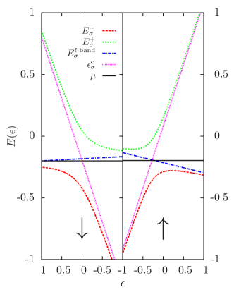
Figure 1: Band structure obtained in mean field approximation, for $P=0.12$, $J_{K}=0.53$, $J_{H}=-0.01$, $n^{c}=0.8$ and $n^{f}_{\text{tot}}=2$.

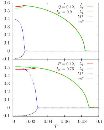
Figure 2: Magnetization of $f$-electrons $M^{f}$, magnetization of $c$-electrons $m^{c}$, and Kondo parameters $\lambda_{\sigma}$ for both spin directions for cases (b) and (c) (see the text for definitions), with $J_{H}=-0.01$, $n^{c}=0.8$ and $n^{f}_{\text{tot}}=2$.

The total Hamiltonian can be now written in the mean field approach as follows:

$${\mathcal{H}} =\sum_{{\bf k}\sigma}\epsilon_{{\bf k}\sigma}^{c}n_{{\bf k}\sigma}^{c}+\sum_{i\sigma\alpha}E_{0\sigma}^{f}n_{i\alpha\sigma}^{f}$$

$$\quad+\sum_{{\bf k}\sigma\alpha}\Lambda_{\sigma}(c_{{\bf k}\sigma}^{\dagger}f_{{\bf k}\alpha\sigma}+h.c.)$$

$$\quad+\sum_{{\bf k}\sigma}A_{{\bf k}\sigma}f_{{\bf k}\alpha\sigma}^{\dagger}f_{{\bf k}\alpha\sigma}+C~{},$$ (25)

where we have :

$$E_{0\sigma}^{f} =E^{f}+U^{\prime}n_{\bar{\sigma}}^{f}+(U^{\prime}-J)n_{\sigma}^{f}+J_{K}\sigma m^{c}$$

$$\quad-\frac{J_{K}}{8}(\lambda_{\uparrow}+\lambda_{\downarrow})^{2}+J_{H}z\sigma M^{f}~{},$$ (26)

$$\epsilon_{{\bf k}\sigma}^{c} =\epsilon_{\bf k}+\Delta_{\sigma}~{},\qquad\Delta_{\sigma}=J_{K}\sigma M^{f}~{},$$ (27)

$$\Lambda_{\sigma} =-\frac{J_{K}}{4}(\lambda_{\sigma}+\lambda_{\bar{\sigma}})~{},$$ (28)

$$C =-2U^{\prime}Nn_{\uparrow}^{f}n_{\downarrow}^{f}-(U^{\prime}-J)N[(n_{\uparrow}^{f})^{2}+(n_{\downarrow}^{f})^{2}]$$

$$\quad+\frac{J_{K}}{2}N(\lambda_{\uparrow}+\lambda_{\downarrow})^{2}-\frac{J_{H}}{2}zN(M^{f})^{2}$$

$$\quad-J_{K}Nm^{c}M^{f}~{},$$ (29)

with $\sigma=\pm\frac{1}{2}$, $M^{f}=n_{\uparrow}^{f}-n_{\downarrow}^{f}$ and $m^{c}=\frac{1}{2}(n_{\uparrow}^{c}-n_{\downarrow}^{c})$.

The diagonalization of the Hamiltonian gives one pure $f$-band, $E^{f}_{{\bf k}\sigma}$ given by :

$$E^{f}_{{\bf k}\sigma}=E_{0\sigma}^{f}+A_{\sigma}\epsilon_{{\bf k}}~{},$$ (30)

and two hybridized bands $E^{\pm}_{{\bf k}\sigma}$ given by:

$$E^{\pm}_{{\bf k}\sigma}=\frac{1}{2}[\epsilon_{{\bf k}}(1+A_{\sigma})+E_{0\sigma}^{f}+\Delta_{\sigma}\pm S_{{\bf k}\sigma}]~{},$$ (31)

with

$$S_{{\bf k}\sigma} =E^{+}_{{\bf k}\sigma}-E^{-}_{{\bf k}\sigma}$$

$$=\sqrt{[\epsilon_{{\bf k}}(1-A_{\sigma})-(E_{0\sigma}^{f}-\Delta_{\sigma})]^{2}+8(\Lambda_{\sigma})^{2}}~{}.$$ (32)

On Fig. 1, we present a typical band structure resulting from the three bands $E^{f}_{{\bf k}\sigma}$ and $E^{\pm}_{{\bf k}\sigma}$ for $J_{K}=0.53$ and $J_{H}=-0.01$. In all figures presented here, $z=6$, where $z$ is the number of nearest neighbors in a simple cubic lattice. In our calculations, the values of $J_{K}$ and $J_{H}$ are defined in units of the half bandwidth $D$ of the conduction band. One can see on Fig. 1 the important effect of the finite $f$-bandwidth: the band structure is very different from that without any $f$-bandwidth used in Ref. Perkins, .

IV RESULTS AND CONCLUSIONS

In this section, we present numerical results obtained from this model, using the general method described in detail in Ref. Perkins, : we derive the Green functions and we calculate self-consistently the magnetization $M^{f}$ for the $f$-electrons, the magnetization $m^{c}$ for the conduction electrons and the two spin-dependent $\lambda_{\sigma}$ parameters which describe the Kondo effect, by imposing constraints on the total number of $f$-electrons and conduction electrons, $n^{f}_{\text{tot}}=2$, and $n^{c}_{\text{tot}}=n^{c}$, respectively. Having solved the self-consistent equations, we study various properties of the model. The Curie and Kondo temperatures are defined, within this mean field approach, as the temperatures at which respectively the magnetizations or the $\lambda_{\sigma}$ parameters tend to zero.

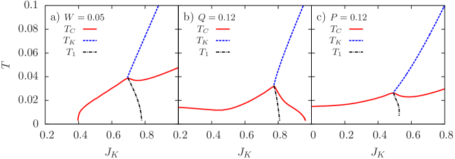
Figure 3: Curie temperature $T_{C}$, and Kondo temperature $T_{K}$, versus $J_{K}$ for the three cases (a), (b) and (c), with $J_{H}=-0.01$, $n^{c}=0.8$ and $n^{f}_{\text{tot}}=2$. For cases (a), (b) and (c) $T_{1}$ is also shown (see the text).

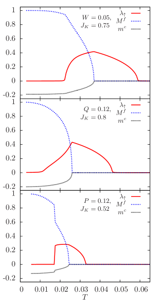
Figure 4: Magnetization of $f$-electrons $M^{f}$, magnetization of $c$-electrons $m^{c}$, and Kondo parameter $\lambda_{\uparrow}$ for cases (a), (b) and (c), with $J_{H}=-0.01$, $n^{c}=0.8$ and $n^{f}_{\text{tot}}=2$. Here $\lambda_{\downarrow}\approx\lambda_{\uparrow}$.

As already mentioned in the previous section, the half $f$-bandwidth derived from the Schrieffer-Wolff transformation is spin-dependent and it is given by $A_{\sigma}$, eq. (24). $A_{\sigma}$ can be rewritten as:

$$A_{\sigma}=-\frac{J_{K}P}{32}\Big{[}7+3(M^{f})^{2}+6\sigma M^{f}\Big{]}~{}.$$ (33)

indicating that the effective bandwidth and the magnetization are correlated. In fact it can be easily checked that the bandwidth for $up$-spin increases with magnetization while it is the opposite for $down$-spin: this is consistent with the double exchange process in the ferromagnetic phase, which favors itinerancy of the conduction electrons with spin parallel to the localized moment, because of intra-atomic Hund’s coupling.

Here, however, we would like to explore the parameter dependence of the effective bandwidth including different possibilities for the relative variation of the Kondo coupling, $J_{K}$, and the $f$-bandwidth $W_{f}$ . In order to do that, we considered also the following definitions of $W_{f}$:

• case (a): a constant bandwidth: $W_{f}=const$;

• case (b): a bandwidth $W_{f}$ proportional to the Kondo coupling constant: $W_{f}=QJ_{K}$; in this way we can take into account the effect of pressure on both the bandwidth and the Kondo coupling, since both are sensitive to the increase of hybridization under pressure.

• case (c): a bandwidth directly obtained from the SW transformation. From Eqs. (23)-(24), we get a spin dependent bandwidth: $W_{f}=2A_{\sigma}$.

In the following, all calculations are done assuming that the conduction band $\epsilon_{\bf k}$ has a width $2D$ and that its density of states is constant and equal to $1/2D$.

On Fig. 2, we present a plot of the temperature variation of the Kondo correlations $\lambda_{\uparrow}$ and $\lambda_{\downarrow}$, and also the $f$ and $c$ magnetizations, $M^{f}$ and $m^{c}$, for cases (b) and (c). The parameters are $n^{c}=0.8$ and $J_{H}=-0.01$. Upper plot is for case (b) with $Q=0.12$, while lower plot is for case (c) with $P=0.12$.

The two magnetization curves clearly show a second order magnetic phase transition at $T_{C}$, below which $m^{c}$ and $M^{f}$ are always antiparallel, as expected because $J_{K}$ is an antiferromagnetic coupling. At low temperatures, Kondo effect and ferromagnetism coexist together, and, due to the breakdown of spin symmetry at $T_{C}$, $\lambda_{\uparrow}$ and $\lambda_{\downarrow}$ become slightly different in the ferromagnetic phase. We define the Kondo temperature as the temperature where $\lambda_{\uparrow}$ and $\lambda_{\downarrow}$ vanish. The fact that the Kondo parameter vanishes at a particular temperature is a well known artefact of the mean field approximation. Actually $T_{K}$ is a crossover temperature, associated with the onset of Kondo screening. In all cases, the Kondo temperature $T_{K}$ is larger than the Curie temperature $T_{C}$ and we never found situations where $T_{K}<T_{C}$: once ferromagnetism is established, Kondo effect does not appear below $T_{C}$; it is blocked by the effective internal magnetic field.

To investigate the effect of the pressure on the Kondo and Curie temperatures, $T_{K}$ and $T_{C}$, respectively, we computed these characteristic temperatures for various values of $J_{K}$ for fixed values of exchange interaction $J_{H}$ and number of conduction electrons $n_{c}$. Figs. 3a,3b and 3c are obtained for three different characterizations of the f-bandwidth, cases (a), (b) and (c), respectively. We notice that the temperatures $T_{K}$ and $T_{C}$ are obtained as the temperatures at which the mean field parameters ($f$ and $c$ magnetizations and the Kondo parameters $\lambda$) vanish. In the three cases we note that the Kondo temperature $T_{K}$ becomes non-zero only above a critical value $J_{K}^{c}$ which varies from case to case. In all cases, once non-zero, the Kondo temperature rapidly increases for larger values of $J_{K}$. The Curie temperature, $T_{C}$, is non-zero above a given $J_{K}$ value in case (a), below a given $J_{K}$ value for case (b) and is non-zero for all studied values of $J_{K}$ for case (c). The reason for these different behaviors is easy to understand. In case a) the f-bandwidth is constant and the system needs a finite value of $J_{K}$ to get magnetic ordering because f-electrons are itinerant even at small $J_{K}$. In case b) the f-bandwidth increases linearly with $J_{K}$, so, for low values of $J_{K}$ the f-electrons are localized and they are magnetic even for $J_{K}=0$; thus as soon as $J_{K}$ is different from zero, magnetic ordering occurs. When increasing $J_{K}$ the f-bandwidth also increases, and magnetism is destroyed because of the itinerant character of the f-electrons. Finally in case c) the f-bandwidth depends on both $J_{K}$ and magnetization, and the dependence is different for up and down spin electrons;it can be seen on figure 3 that this complex dependence of the bandwidth leads to small variation of the Curie temperature, with a weak maximum. However a crossing point, at which $T_{C}$ and $T_{K}$ are equal is obtained in all cases.

Concerning the Kondo effect, in all cases (a), (b) and (c) a peculiar behavior has been obtained for values of $J_{K}$ just above this crossing point: at the temperature $T_{1}$ indicated on Fig. 3a), 3b) and 3c) the Kondo parameters vanish, being non-zero only between $T_{1}$ and $T_{K}$. To better understand this behavior, we have plotted on Fig. 4, $M^{f}$, $m^{c}$ and $\lambda_{\uparrow}$ for $n^{c}=0.8$, $J_{H}=-0.01$ but for values of $J_{K}$ near the crossing of $T_{C}$ and $T_{K}$, i.e., $J_{K}=0.75$ for case (a), $J_{K}=0.8$ for case (b) and $J_{K}=0.52$ for case (c). It appears clearly that, with decreasing temperature, the Kondo effect occurs first, then there is a coexistence of Kondo effect and ferromagnetism, and finally the Kondo effect disappears to yield only a strong ferromagnetism at extremely low temperatures. This behavior can be interpreted in the following way: Kondo effect for a spin $S=1$ cannot be complete, as explained in the introduction. Thus if exchange is large enough, the ordering of the remaining $f$-moments occurs in the Kondo phase. However, at lower temperature, when these magnetic moments are large, they act as an internal magnetic field that destroys the Kondo effect. It should be pointed out that there is at present no experimental evidence in favor or in contrast of such an effect in actinide compounds at very low temperature.

Another interesting result that can be pointed out is the decrease of the Curie temperature for large $J_{K}$ above the intersection point particularly in case (b), but also within a small range of value of $J_{K}$ in case (c). This decrease can probably be considered as resulting from the ”delocalization” of the 5$f$-electrons. Let us also remark that $J_{K}$ increases with increasing pressure and that the two Figs. 3b) and 3c) can give a description of the experimentally observed variation of $T_{C}$ with pressure in UTe compound, which is passing through a maximum and then decreasing with applied pressure.Schoenes3 ; Cooper

To summarize our paper, the present work improves the previous $S=1$ UKL model of Ref. Perkins, by explicitly including the effect of a weak delocalization of the $5f$-electrons. Within this improved model, we have obtained new phenomena in the region where $T_{C}$ and $T_{K}$ are of the same order of magnitude: a possible disappearance of the Kondo effect at low temperature, which is a direct consequence of the underscreened Kondo effect, and a maximum of $T_{C}$ as a function of $J_{K}$. It is worth to note that, in our model, the delocalization of the $5f$-electrons increases when $J_{K}$ increases, i.e. when pressure is applied; then the magnetization decreases and in the same way the Curie temperature. Therefore, the change in the Curie temperature at large $J_{K}$ is more influenced by delocalization than by competition between magnetism and Kondo effect. This is a different result compared with the case of Cerium compounds, where the magnetization is destroyed by Kondo effect, i.e. by the screening of the magnetic moment. In the underscreened $S=1$ Kondo lattice, because Kondo screening can never be complete, the Kondo effect alone does not destroy ferromagnetism.

To conclude, we have shown that our model includes two effects which are essential to describe the $5f$-electron compounds: the small delocalization of the $5f$-electrons, and the $S=1$ spins found in uranium or neptunium compounds. The first effect works against magnetism, while the second one favors magnetism. The competition between these two effects leads to complex phase diagrams which can improve the description of some actinide compounds and explain in particular the maximum of $T_{C}$ observed experimentally in UTe compound with increasing pressure.

- (1) A. C. Hewson The Kondo problem to Heavy Fermions, Cambridge University Press (1993).
- (2) B. Coqblin, AIP Conference Procedings, volume 846, pp. 3-93 (2006).
- (3) G. R. Stewart, Rev. Mod. Phys. 56, 755 (1984).
- (4) B. Coqblin, J.R. Iglesias-Sicardi and R. Jullien, Contemporary Physics 19, 327 (1978).
- (5) Q. G. Sheng and B. R. Cooper, J. Magn. Magn. Mater. 164, 335 (1996).
- (6) B. R. Cooper and Y.-L. Lin, J. Appl. Phys. 83, 6432 (1998).
- (7) E. M. Collins, N. Kioussis, S. P. Lim, and B. R. Cooper, J. Appl. Phys. 85, 6226 (1999).
- (8) G. Zwicknagl, A. N. Yaresko and P. Fulde, Phys. Rev. B 65, 081103(R) (2002).
- (9) G. Zwicknagl, A. N. Yaresko and P. Fulde, Phys. Rev. B 68, 052508 (2003).
- (10) K. T. Moore and G. van der Laan, Rev. Mod. Phys. 81, 235 (2009).
- (11) P. Santini, S. Carretta, G. Amoretti, R. Caciuffo, N. Magnani, and G. H. Lander Rev. Mod. Phys. 81, 807 (2009).
- (12) B. Coqblin, M. D. Nunez-Regueiro, Alba Theumann, J.R. Iglesias and S.G. Magalhaes, Philosophical Magazine 86, 2567 (2006).
- (13) S. Doniach, Proceedings of the “Int. Conf. on Valence Instabilities and Related Narrow-band Phenomena”, ed. By R. D. Parks, Plenum Press, 168 (1976).
- (14) J. Schoenes, J. Less-Common Met., 121, 87 (1986).
- (15) J. Schoenes, B. Frick, and O. Vogt, Phys. Rev. B 30, 6578 (1984).
- (16) J. Schoenes, O. Vogt, J. Lohle, F. Hulliger, and K. Mattenberger, Phys. Rev. B 53, 14987 (1996)
- (17) Z. Bukowski, R. Troc, J. Stepien-Damm, C. Sulkowski and V. H. Tran, J. Alloys and Compounds, 403, 65 (2005).
- (18) V. H. Tran, R. Troc, Z. Bukowski, D. Badurski and C. Sulkowski, Phys. Rev. B 71, 094428 (2005).
- (19) E. Colineau, F. Wastin, J.P. Sanchez and J. Rebizant, J. Phys.: Cond. Matter, 20, 075207 (2008).
- (20) V. H. Tran, J. C. Griveau, R. Eloirdi, W. Miiller and E. Colineau, presented at the 40 emes Journees des Actinides, Geneva, Switzerland, March 2010.
- (21) P. Nozieres and A. Blandin, J. de Physique 41, 193 (1980)
- (22) K. Le Hur and B. Coqblin, Phys. Rev. B 56, 668 (1997).
- (23) O. Parcollet and A. Georges, Phys. Rev. Lett. 79, 4665 (1997)
- (24) S. Florens, Phys. Rev. B 70, 165112 (2004)
- (25) P. Coleman and I. Paul, Phys. Rev. B 71, 035111 (2005)
- (26) P. Schlottmann and P. D. Sacramento, Adv. in Phys. 42, 641 (1993).
- (27) M. Pustilnik and L.I. Glazman, Phys. Rev. Lett. 87, 216601 (2001)
- (28) I. Weymann, L. Borda, Phys. Rev. B 81, 115445 (2010); L. Borda, M. Garst, J. Kroha, Phys. Rev. B 79, 100408(R) (2009)
- (29) N. Roch, S. Florens, T. A. Costi, W. Wernsdorfer, F. Balestro, Phys. Rev. Lett. 103, 197202 (2009)
- (30) N. B. Perkins, M. D. Núñez-Regueiro, B. Coqblin and J. R. Iglesias, Phys. Rev. B 76, 125101 (2007).
- (31) S. Di Matteo, N.B. Perkins and C.R Natoli, Phys. Rev. B 65, 054413 (2002).
- (32) J.R. Schrieffer and P.A. Wolff, Phys. Rev. 149 , 491 (1966)
- (33) Christopher Thomas, Acirete S. da R. Simoes, C. Lacroix, J. R. Iglesias and B. Coqblin, presented at SCES 2008 Conference, Buzios, Brazil (August 2008), Physica B 404, 3008 (2009).
- (34) A. Yoshimori and A. Sakurai, Prog. Theo. Phys. Suppl. 46, 162 (1970).
- (35) C. Lacroix and M. Cyrot, Phys. Rev. B 20, 1969 (1979).
- (36) P. Coleman and N. Andrei, J. Phys.: Condens. Matter 1, 4057 (1989).