A Self-Organising Neural Network for Processing Data from Multiple Sensors

Abstract

This paper shows how a folded Markov chain network can be applied to the problem of processing data from multiple sensors, with an emphasis on the special case of 2 sensors. It is necessary to design the network so that it can transform a high dimensional input vector into a posterior probability, for which purpose the partitioned mixture distribution network is ideally suited. The underlying theory is presented in detail, and a simple numerical simulation is given that shows the emergence of ocular dominance stripes.

1 Theory

1.1 Neural Network Model

In order to fix ideas, it is useful to give an explicit “neural network” interpretation to the theory that will be developed. The model will consist of 2 layers of nodes. The input layer has a “pattern of activity” that represents the components of the input vector $\mathbf{x}$, and the output layer has a pattern of activity that is the collection of activities of each output node. The activities in the output layer depend only on the activities in the input layer. If an input vector $\mathbf{x}$ is presented to this network, then each output node “fires” discretely at a rate that corresponds to its activity. After $n$ nodes have fired the probabilistic description of the relationship between the input and output of the network is given by $\Pr\left(\mathbf{y}_{1},\mathbf{y}_{2},\cdots,\mathbf{y}_{n}|\mathbf{x}\right)$, where $\mathbf{y}_{i}$ is the location in the output layer (assumed to be on a rectangular lattice of size $\mathbf{m}$) of the $i^{th}$ node that fires. In this paper it will be assumed that the order in which the $n$ nodes fire is not observed, in which case $\Pr\left(\mathbf{y}_{1},\mathbf{y}_{2},\cdots,\mathbf{y}_{n}|\mathbf{x}\right)$ is a sum of probabilities over all $n!$ permutations of $\left(\mathbf{y}_{1},\mathbf{y}_{2},\cdots,\mathbf{y}_{n}\right)$, which is a symmetric function of the $\mathbf{y}_{i}$, by construction.

The theory that is introduced in section 1.2 concerns the special case $n=1$. In the $n=1$ case the probabilistic description $\Pr\left(\mathbf{y|x}\right)$ is proportional to the firing rate of node $\mathbf{y}$ in response to input $\mathbf{x}$. When $n>1$ there is an indirect relationship between the probabilistic description $\Pr\left(\mathbf{y}_{1},\mathbf{y}_{2},\cdots,\mathbf{y}_{n}|\mathbf{x}\right)$ and the firing rate of node $\mathbf{y}$, which is given by the marginal probability

$$\Pr\left(\mathbf{y|x}\right)=\sum_{\mathbf{y}_{2},\cdots,\mathbf{y}_{n}}^{\mathbf{m}}\Pr\left(\mathbf{y},\mathbf{y}_{2},\cdots,\mathbf{y}_{n}|\mathbf{x}\right)$$ (1)

It is important to maintain this distinction between events that are observed (i.e. $\left(\mathbf{y}_{1},\mathbf{y}_{2},\cdots,\mathbf{y}_{n}\right)$ given $\mathbf{x}$) and the probabilistic description of the events that are observed (i.e. $\Pr\left(\mathbf{y}_{1},\mathbf{y}_{2},\cdots,\mathbf{y}_{n}|\mathbf{x}\right)$). The only possible exception is in the $n\rightarrow\infty$ limit, where $\Pr\left(\mathbf{y}_{1},\mathbf{y}_{2},\cdots,\mathbf{y}_{n}|\mathbf{x}\right)$ has all of its probability concentrated in the vicinity of those $\left(\mathbf{y}_{1},\mathbf{y}_{2},\cdots,\mathbf{y}_{n}\right)$ that are consistent with the observed long-term average firing rate of each node. It is essential to consider the $n>1$ case to obtain the results that are described in this paper.

1.2 Probabilistic Encoder/Decoder

A theory of self-organising networks based on an analysis of a probabilistic encoder/decoder was presented in [1]. It deals with the $n=1$ case referred to in section 1.1. The objective function that needs to be minimised in order to optimise a network in this theory is the Euclidean distortion $D$ defined as

$$D\equiv\sum_{\mathbf{y}=\mathbf{1}}^{\mathbf{m}}\int d\mathbf{x}\,d\mathbf{x}^{\prime}\Pr\left(\mathbf{x}\right)\Pr\left(\mathbf{y}|\mathbf{x}\right)\Pr\left(\mathbf{x}^{\prime}\mathbf{|y}\right)\left\|\mathbf{x}-\mathbf{x}^{\prime}\right\|^{2}$$ (2)

where $\mathbf{x}$ is an input vector, $\mathbf{y}$ is a coded version of $\mathbf{x}$ (a vector index on a $d$-dimensional rectangular lattice of size $\mathbf{m}$), $\mathbf{x}^{\prime}$ is a reconstructed version of $\mathbf{x}$ from $\mathbf{y}$, $\Pr\left(\mathbf{x}\right)$ is the probability density of input vectors, $\Pr\left(\mathbf{y}|\mathbf{x}\right)$ is a probabilistic encoder, and $\Pr\left(\mathbf{x}^{\prime}\mathbf{|y}\right)$ is a probabilistic decoder which is specified by Bayes’ theorem as

$$\Pr\left(\mathbf{x|y}\right)=\frac{\Pr\left(\mathbf{y}|\mathbf{x}\right)\Pr\left(\mathbf{x}\right)}{\int d\mathbf{x}^{\prime}\Pr\left(\mathbf{y}|\mathbf{x}^{\prime}\right)\Pr\left(\mathbf{x}^{\prime}\right)}$$ (3)

$D$ can be rearranged into the form [1]

$$D=2\sum_{\mathbf{y}=\mathbf{1}}^{\mathbf{m}}\int d\mathbf{x}\Pr\left(\mathbf{x}\right)\Pr\left(\mathbf{y}|\mathbf{x}\right)\left\|\mathbf{x}-\mathbf{x}^{\prime}\left(\mathbf{y}\right)\right\|^{2}$$ (4)

where the reference vectors $\mathbf{x}^{\prime}\left(\mathbf{y}\right)$ are defined as

$$\mathbf{x}^{\prime}\left(\mathbf{y}\right)\equiv\int d\mathbf{x}\Pr\left(\mathbf{x|y}\right)\,\mathbf{x}$$ (5)

Although equation 2 is symmetric with respect to interchanging the encoder and decoder, equation 4 is not. This is because Bayes’ theorem has made explicit the dependence of $\Pr\left(\mathbf{x|y}\right)$ on $\Pr\left(\mathbf{y}|\mathbf{x}\right)$. From a neural network viewpoint $\Pr\left(\mathbf{y}|\mathbf{x}\right)$ describes the feed-forward transformation from the input layer to the output layer, and $\mathbf{x}^{\prime}\left(\mathbf{y}\right)$ describes the feed-back transformation that is implied from the output layer to the input layer. The feed-back transformation is necessary to implement the objective function that has been chosen here.

Minimisation of $D$ with respect to all free parameters leads to an optimal encoder/decoder. In equation 4 the $\Pr\left(\mathbf{y}|\mathbf{x}\right)$ are the only free parameters, because $\mathbf{x}^{\prime}\left(\mathbf{y}\right)$ is fixed by equation 5. However, in practice, both $\Pr\left(\mathbf{y}|\mathbf{x}\right)$ and $\mathbf{x}^{\prime}\left(\mathbf{y}\right)$ may be treated as free parameters [1], because $\mathbf{x}^{\prime}\left(\mathbf{y}\right)$ satisfy equation 5 at stationary points of $D$ with respect to variation of $\mathbf{x}^{\prime}\left(\mathbf{y}\right)$.

1.3 Posterior Probability Model

The probabilistic encoder/decoder requires an explicit functional form for the posterior probability $\Pr\left(\mathbf{y}|\mathbf{x}\right)$. A convenient expression is

$$\Pr\left(\mathbf{y}|\mathbf{x}\right)=\frac{Q\left(\mathbf{x}|\mathbf{y}\right)}{\sum_{\mathbf{y}^{\prime}=\mathbf{1}}^{\mathbf{m}}Q\left(\mathbf{x}|\mathbf{y}^{\prime}\right)}$$ (6)

where $Q\left(\mathbf{x}|\mathbf{y}\right)>0$ can be regarded as a node “activity”, and $\sum_{\mathbf{y}=\mathbf{1}}^{\mathbf{m}}P\left(\mathbf{y}|\mathbf{x}\right)=1$. Any non-negative function can be used for $Q\left(\mathbf{x}|\mathbf{y}\right)$, such as a sigmoid (which satisfies $0\leq Q\left(\mathbf{x}|\mathbf{y}\right)\leq 1$)

$$Q\left(\mathbf{x}|\mathbf{y}\right)=\frac{1}{1+\exp\left(-\mathbf{w}\left(\mathbf{y}\right)\cdot\mathbf{x}-b\left(\mathbf{y}\right)\right)}$$ (7)

where $\mathbf{w}\left(\mathbf{y}\right)$ and $b\left(\mathbf{y}\right)$ are a weight vector and bias, respectively.

A drawback to the use of equation 6 is that it does not permit it to scale well to input vectors that have a large dimensionality. This problem arises from the restricted functional form allowed for $Q\left(\mathbf{x}|\mathbf{y}\right)$. A solution was presented in [2]

$$\Pr\left(\mathbf{y}|\mathbf{x}\right)=\frac{1}{M}\,Q\left(\mathbf{x}|\mathbf{y}\right)\sum_{\mathbf{y}^{\prime}\in\tilde{N}\left(\mathbf{y}\right)}\frac{1}{\sum_{\mathbf{y}^{\prime\prime}\in N\left(\mathbf{y}^{\prime}\right)}Q\left(\mathbf{x}|\mathbf{y}^{\prime\prime}\right)}$$ (8)

where $M\equiv m_{1}m_{2}\cdots m_{d}$, and $N\left(\mathbf{y}\right)$ is a set of lattice points that are deemed to be “in the neighbourhood of” the lattice point $\mathbf{y}$, and $\tilde{N}\left(\mathbf{y}\right)$ is the inverse neighbourhood defined as the set of lattice points that have lattice point $\mathbf{y}$ in their neighbourhood. This expression for $\Pr\left(\mathbf{y}|\mathbf{x}\right)$ satisfies $\sum_{\mathbf{y}=1}^{\mathbf{m}}P\left(\mathbf{y}|\mathbf{x}\right)=1$ (see appendix A). It is convenient to define

$$\Pr\left(\mathbf{y}|\mathbf{x};\mathbf{y}^{\prime}\right)\equiv\frac{Q\left(\mathbf{x}|\mathbf{y}\right)}{\sum_{\mathbf{y}^{\prime\prime}\in N\left(\mathbf{y}^{\prime}\right)}Q\left(\mathbf{x}|\mathbf{y}^{\prime\prime}\right)}$$ (9)

which is another posterior probability, by construction. It includes the effect of the output nodes that are in the neighbourhood of node $\mathbf{y}^{\prime}$ only. $\Pr\left(\mathbf{y}|\mathbf{x};\mathbf{y}^{\prime}\right)$ is thus a localised posterior probability derived from a localised subset of the node activities. This allows equation 8 to be written as $\Pr\left(\mathbf{y}|\mathbf{x}\right)=\frac{1}{M}\sum_{\mathbf{y}^{\prime}\in\tilde{N}\left(\mathbf{y}\right)}\Pr\left(\mathbf{y}|\mathbf{x};\mathbf{y}^{\prime}\right)$, so $\Pr\left(\mathbf{y}|\mathbf{x}\right)$ is the average of the posterior probabilities at node $\mathbf{y}$ arising from each of the localised subsets that happens to include node $\mathbf{y}$.

1.4 Multiple Firing Model

The model may be extended to the case where $n$ output nodes fire. $\Pr\left(\mathbf{y}|\mathbf{x}\right)$ is then replaced by $\Pr\left(\mathbf{y}_{1},\mathbf{y}_{2},\cdots\mathbf{y}_{n}|\mathbf{x}\right)$, which is the probability that $\left(\mathbf{y}_{1},\mathbf{y}_{2},\cdots\mathbf{y}_{n}\right)$ are the first $n$ nodes to fire (in that order). With this modification, $D$ becomes

$$D=2\sum_{\mathbf{y}_{1},\mathbf{y}_{2},\cdots\mathbf{y}_{n}=\mathbf{1}}^{\mathbf{m}}\int d\mathbf{x}\Pr\left(\mathbf{x}\right)\Pr\left(\mathbf{y}_{1},\mathbf{y}_{2},\cdots\mathbf{y}_{n}|\mathbf{x}\right)\left\|\mathbf{x}-\mathbf{x}^{\prime}\left(\mathbf{y}_{1},\mathbf{y}_{2},\cdots\mathbf{y}_{n}\right)\right\|^{2}$$ (10)

where the reference vectors $\mathbf{x}^{\prime}\left(\mathbf{y}_{1},\mathbf{y}_{2},\cdots\mathbf{y}_{n}\right)$ are defined as

$$\mathbf{x}^{\prime}\left(\mathbf{y}_{1},\mathbf{y}_{2},\cdots\mathbf{y}_{n}\right)\equiv\int d\mathbf{x}\Pr\left(\mathbf{x|y}_{1},\mathbf{y}_{2},\cdots\mathbf{y}_{n}\right)\,\mathbf{x}$$ (11)

The dependence of $\Pr\left(\mathbf{y}_{1},\mathbf{y}_{2},\cdots\mathbf{y}_{n}|\mathbf{x}\right)$ and $\mathbf{x}^{\prime}\left(\mathbf{y}_{1},\mathbf{y}_{2},\cdots\mathbf{y}_{n}\right)$ on $n$ output node locations complicates this result. Assume that $\Pr\left(\mathbf{y}_{1},\mathbf{y}_{2},\cdots\mathbf{y}_{n}|\mathbf{x}\right)$ is a symmetric function of its $\left(\mathbf{y}_{1},\mathbf{y}_{2},\cdots\mathbf{y}_{n}\right)$ arguments, which corresponds to ignoring the order in which the first $n$ nodes choose to fire (i.e. $\Pr\left(\mathbf{y}_{1},\mathbf{y}_{2},\cdots\mathbf{y}_{n}|\mathbf{x}\right)$ is a sum over all permutations of $\left(\mathbf{y}_{1},\mathbf{y}_{2},\cdots\mathbf{y}_{n}\right)$). For simplicity, assume that the nodes fire independently so that $\Pr\left(\mathbf{y}_{1},\mathbf{y}_{2}|\mathbf{x}\right)=\Pr\left(\mathbf{y}_{1}|\mathbf{x}\right)\Pr\left(\mathbf{y}_{2}|\mathbf{x}\right)$ (see appendix B for the general case where $\Pr\left(\mathbf{y}_{1},\mathbf{y}_{2}|\mathbf{x}\right)$ does not factorise). $D$ may be shown to satisfy the inequality $D\leq D_{1}+D_{2}$ (see appendix B), where

$$D_{1} \equiv \frac{2}{n}\sum_{\mathbf{y}=1}^{\mathbf{m}}\int d\mathbf{x}\Pr\left(\mathbf{x}\right)\Pr\left(\mathbf{y}|\mathbf{x}\right)\left\|\mathbf{x}-\mathbf{x}^{\prime}\left(\mathbf{y}\right)\right\|^{2}$$

$$D_{2} \equiv \frac{2\left(n-1\right)}{n}\int d\mathbf{x}\Pr\left(\mathbf{x}\right)\left\|\sum_{\mathbf{y}=\mathbf{1}}^{\mathbf{m}}\Pr\left(\mathbf{y}|\mathbf{x}\right)\left(\mathbf{x}-\mathbf{x}^{\prime}\left(\mathbf{y}\right)\right)\right\|^{2}$$ (12)

$D_{1}$ and $D_{2}$ are both non-negative. $D_{1}\rightarrow 0$ as $n\rightarrow\infty$, and $D_{2}=0$ when $n=0$, so the $D_{1}$ term is the sole contribution to the upper bound when $n=0$, and the $D_{2}$ term provides the dominant contribution as $n\rightarrow\infty$. The difference between the $D_{1}$ and the $D_{2}$ terms is the location of the $\sum_{\mathbf{y}=\mathbf{1}}^{\mathbf{m}}\Pr\left(\mathbf{y}|\mathbf{x}\right)\left(\cdots\right)$ average: in the $D_{2}$ term it averages a vector quantity, whereas in the $D_{1}$ term it averages a Euclidean distance. The $D_{2}$ term will therefore exhibit interference effects, whereas the $D_{1}$ term will not.

1.5 Probability Leakage

The model may be further extended to the case where the probability that a node fires is a weighted average of the underlying probabilities that the nodes in its vicinity fire. Thus $\Pr\left(\mathbf{y}|\mathbf{x}\right)$ becomes

$$\Pr\left(\mathbf{y}|\mathbf{x}\right)\rightarrow\sum_{\mathbf{y}^{\prime}=\mathbf{1}}^{\mathbf{m}}\Pr\left(\mathbf{y}|\mathbf{y}^{\prime}\right)\Pr\left(\mathbf{y}^{\prime}|\mathbf{x}\right)$$ (13)

where $\Pr\left(\mathbf{y}|\mathbf{y}^{\prime}\right)$ is the conditional probability that node $\mathbf{y}$ fires given that node $\mathbf{y}^{\prime}$ would have liked to fire. In a sense, $\Pr\left(\mathbf{y}|\mathbf{y}^{\prime}\right)$ describes a “leakage” of probability from node $\mathbf{y}^{\prime}$ that onto node $\mathbf{y}$. $\Pr\left(\mathbf{y}|\mathbf{y}^{\prime}\right)$ then plays the role of a soft “neighbourhood function” for node $\mathbf{y}^{\prime}$. This expression for $\Pr\left(\mathbf{y}|\mathbf{x}\right)$ can be used wherever a plain $\Pr\left(\mathbf{y}|\mathbf{x}\right)$ has been used before. The main purpose of introducing leakage is to encourage neighbouring nodes to perform a similar function. This occurs because the effect of leakage is to soften the posterior probability $\Pr\left(\mathbf{y}|\mathbf{x}\right)$, and thus reduce the ability to reconstruct $\mathbf{x}$ accurately from knowledge of $\mathbf{y}$, which thus increases the average Euclidean distortion $D$. To reduce the damage that leakage causes, the optimisation must ensure that nodes that leak probability onto each other have similar properties, so that it does not matter much that they leak.

1.6 The Model

The focus of this paper is on minimisation of the upper bound $D_{1}+D_{2}$ (see equation 12) to $D$ in the multiple firing model, using a scalable posterior probability $\Pr\left(\mathbf{y}|\mathbf{x}\right)$ (see equation 8), with the effect of activity leakage $\Pr\left(\mathbf{y}|\mathbf{y}^{\prime}\right)$ taken into account (see equation 13). Gathering all of these pieces together yields

$$D_{1} = \frac{2}{n\,M}\int d\mathbf{x}\Pr\left(\mathbf{x}\right)\sum_{\mathbf{y}=\mathbf{1}}^{\mathbf{m}}\sum_{\mathbf{y}^{\prime}=\mathbf{1}}^{\mathbf{m}}\Pr\left(\mathbf{y}|\mathbf{y}^{\prime}\right)\sum_{\mathbf{y}^{\prime\prime}\in\tilde{N}\left(\mathbf{y}^{\prime}\right)}\Pr\left(\mathbf{y}^{\prime}|\mathbf{x};\mathbf{y}^{\prime\prime}\right)\left\|\mathbf{x}-\mathbf{x}^{\prime}\left(\mathbf{y}\right)\right\|^{2}$$

$$D_{2} = \frac{2\left(n-1\right)}{n\,M^{2}}\int d\mathbf{x}\Pr\left(\mathbf{x}\right)$$

$$\times\left\|\sum_{\mathbf{y}=\mathbf{1}}^{\mathbf{m}}\sum_{\mathbf{y}^{\prime}=\mathbf{1}}^{\mathbf{m}}\Pr\left(\mathbf{y}|\mathbf{y}^{\prime}\right)\sum_{\mathbf{y}^{\prime\prime}\in\tilde{N}\left(\mathbf{y}^{\prime}\right)}\Pr\left(\mathbf{y}^{\prime}|\mathbf{x};\mathbf{y}^{\prime\prime}\right)\left(\mathbf{x}-\mathbf{x}^{\prime}\left(\mathbf{y}\right)\right)\right\|^{2}$$

where $\Pr\left(\mathbf{y}|\mathbf{x};\mathbf{y}^{\prime}\right)\equiv\frac{Q\left(\mathbf{x}|\mathbf{y}\right)}{\sum_{\mathbf{y}^{\prime\prime}\in N\left(\mathbf{y}^{\prime}\right)}Q\left(\mathbf{x}|\mathbf{y}^{\prime\prime}\right)}$.

In order to ensure that the model is truly scalable, it is necessary to restrict the dimensionality of the reference vectors. In equation 1.6 $\dim\mathbf{x}^{\prime}\left(\mathbf{y}\right)=\dim\mathbf{x}$, which is not acceptable in a scalable network. In practice, it will be assumed any properties of node $\mathbf{y}$ that are vectors in input space will be limited to occupy an “input window” of restricted size that is centred on node $\mathbf{y}$. This restriction applies to the node reference vector $\mathbf{x}^{\prime}\left(\mathbf{y}\right)$, which prevents $D_{1}+D_{2}$ from being fully minimised, because $\mathbf{x}^{\prime}\left(\mathbf{y}\right)$ is allowed to move only in a subspace of the full-dimensional input space. However, useful results can nevertheless be obtained, so this restriction is acceptable.

1.7 Optimisation

Optimisation is achieved by minimising $D_{1}+D_{2}$ with respect to its free parameters. Thus the derivatives with respect to $\mathbf{x}^{\prime}\left(\mathbf{y}\right)$ are given by

$$\frac{\partial D_{1}}{\partial\mathbf{x}^{\prime}\left(\mathbf{y}\right)} = -\frac{4}{n\,M}\int d\mathbf{x}\Pr\left(\mathbf{x}\right)\,\mathbf{f}_{1}\left(\mathbf{x},\mathbf{y}\right)$$

$$\frac{\partial D_{2}}{\partial\mathbf{x}^{\prime}\left(\mathbf{y}\right)} = -\frac{4\left(n-1\right)}{n\,M^{2}}\int d\mathbf{x}\Pr\left(\mathbf{x}\right)\,\mathbf{f}_{2}\left(\mathbf{x},\mathbf{y}\right)$$ (15)

and the variations with respect to $Q\left(\mathbf{x}|\mathbf{y}\right)$ are given by

$$\delta D_{1} = \frac{2}{n\,M}\sum_{\mathbf{y}=\mathbf{1}}^{\mathbf{m}}\int d\mathbf{x}\Pr\left(\mathbf{x}\right)\,g_{1}\left(\mathbf{x},\mathbf{y}\right)\,\delta\log Q\left(\mathbf{x}|\mathbf{y}\right)$$

$$\delta D_{2} = \frac{4\left(n-1\right)}{n\,M^{2}}\sum_{\mathbf{y}=\mathbf{1}}^{\mathbf{m}}\int d\mathbf{x}\Pr\left(\mathbf{x}\right)\,g_{2}\left(\mathbf{x},\mathbf{y}\right)\,\delta\log Q\left(\mathbf{x}|\mathbf{y}\right)$$ (16)

The functions $\mathbf{f}_{1}\left(\mathbf{x},\mathbf{y}\right)$, $\,\mathbf{f}_{2}\left(\mathbf{x},\mathbf{y}\right)$, $g_{1}\left(\mathbf{x},\mathbf{y}\right)$, and $g_{2}\left(\mathbf{x},\mathbf{y}\right)$ are derived in appendix C. Inserting a sigmoidal function $Q\left(\mathbf{x}|\mathbf{y}\right)=\frac{1}{1+\exp\left(-\mathbf{w}\left(\mathbf{y}\right)\cdot\mathbf{x}-b\left(\mathbf{y}\right)\right)}$ then yields the derivatives with respect to $\mathbf{w}\left(\mathbf{y}\right)$ and $b\left(\mathbf{y}\right)$ as

$$\frac{\partial D_{1}}{\partial\left(\begin{array}[]{c}b\left(\mathbf{y}\right)\\ \mathbf{w}\left(\mathbf{y}\right)\end{array}\right)} = \frac{2}{n\,M}\int d\mathbf{x}\Pr\left(\mathbf{x}\right)\,g_{1}\left(\mathbf{x},\mathbf{y}\right)\,\left(1-Q\left(\mathbf{x}|\mathbf{y}\right)\right)\left(\begin{array}[]{c}1\\ \mathbf{x}\end{array}\right)$$ (21)

$$\frac{\partial D_{2}}{\partial\left(\begin{array}[]{c}b\left(\mathbf{y}\right)\\ \mathbf{w}\left(\mathbf{y}\right)\end{array}\right)} = \frac{4\left(n-1\right)}{n\,M^{2}}\int d\mathbf{x}\Pr\left(\mathbf{x}\right)\,g_{2}\left(\mathbf{x},\mathbf{y}\right)\,\,\left(1-Q\left(\mathbf{x}|\mathbf{y}\right)\right)\left(\begin{array}[]{c}1\\ \mathbf{x}\end{array}\right)$$ (26)

Because all of the properties of node $\mathbf{y}$ that are vectors in input space (i.e. $\mathbf{x}^{\prime}\left(\mathbf{y}\right)$ and $\mathbf{w}\left(\mathbf{y}\right)$) are assumed to be restricted to an input window centred on node $\mathbf{y}$, the eventual result of evaluating the right hand sides of the above equations must be similarly restricted to the same input window.

1.8 The Effect of the Euclidean Norm on Minimising $D_{1}+D_{2}$

The expressions for $D_{1}$ and $D_{2}$, and especially their derivatives, are fairly complicated, so an intuitive interpretation will now be presented. When $D_{1}+D_{2}$ is stationary with respect to variations of $\mathbf{x}^{\prime}\left(\mathbf{y}\right)$ it may be written as (see appendix D).

$$\begin{array}[]{lll}D_{1}+D_{2}&=&-\frac{2}{n}\int d\mathbf{x}\Pr\left(\mathbf{x}\right)\sum_{\mathbf{y}=\mathbf{1}}^{\mathbf{m}}\Pr\left(\mathbf{y}|\mathbf{x}\right)\left\|\mathbf{x}^{\prime}\left(\mathbf{y}\right)\right\|^{2}\\ \\ &&-\frac{2\left(n-1\right)}{n}\int d\mathbf{x}\Pr\left(\mathbf{x}\right)\left\|\sum_{\mathbf{y}=\mathbf{1}}^{\mathbf{m}}\Pr\left(\mathbf{y}|\mathbf{x}\right)\mathbf{x}^{\prime}\left(\mathbf{y}\right)\right\|^{2}\\ \\ &&+\text{ constant}\end{array}$$ (27)

The $M$ and $M^{2}$ factors do not appear in this expression because $\Pr\left(\mathbf{y}|\mathbf{x}\right)$ is normalised to sum to unity. The first term (which derives from $D_{1}$) is an incoherent sum (i.e. a sum of Euclidean distances), whereas the second term (which derives from $D_{2}$) is a coherent sum (i.e. a sum of vectors). The first term contributes for all values of $n$, whereas the second term contributes only for $n\geq 2$, and dominates for $n\gg 1$. In order to minimise the first term the $\left\|\mathbf{x}^{\prime}\left(\mathbf{y}\right)\right\|^{2}$ like to be as large as possible for those nodes that have a large $\Pr\left(\mathbf{y}|\mathbf{x}\right)$. Since $\mathbf{x}^{\prime}\left(\mathbf{y}\right)$ is the centroid of the probability density $\Pr\left(\mathbf{x}|\mathbf{y}\right)$, this implies that node $\mathbf{y}$ prefers to encode a region of input space that is as far as possible from the origin. This is a consequence of using a Euclidean distortion measure $\left\|\mathbf{x-x}^{\prime}\right\|^{2}$, which has the dimensions of $\left\|\mathbf{x}\right\|^{2}$, in the original definition of the distortion in equation 2. In order to minimise the second term the superposition of $\mathbf{x}^{\prime}\left(\mathbf{y}\right)$ weighted by the $\Pr\left(\mathbf{y}|\mathbf{x}\right)$ likes to have as large a Euclidean norm as possible. Thus the nodes co-operate amongst themselves to ensure that the nodes that have a large $\Pr\left(\mathbf{y}|\mathbf{x}\right)$ also have a large $\left\|\sum_{\mathbf{y}=\mathbf{1}}^{\mathbf{m}}\Pr\left(\mathbf{y}|\mathbf{x}\right)\mathbf{x}^{\prime}\left(\mathbf{y}\right)\right\|^{2}$.

2 Solvable Analytic Model

The purpose of this section is to work through a case study in order to demonstrate the various properties that emerge when $D_{1}+D_{2}$ is minimised.

2.1 The Model

It convenient to begin by ignoring the effects of leakage $\Pr\left(\mathbf{y|y}^{\prime}\right)$, and to concentrate on a simple (non-scaling) version of the posterior probability model (as in equation 6) $\Pr\left(\mathbf{y}|\mathbf{x}\right)=\frac{Q\left(\mathbf{x}|\mathbf{y}\right)}{\sum_{\mathbf{y}^{\prime}=1}^{\mathbf{m}}Q\left(\mathbf{x}|\mathbf{y}^{\prime}\right)}$, where the $Q\left(\mathbf{x|y}\right)$ are threshold functions of $\mathbf{x}$

$$Q\left(\mathbf{x|y}\right)=\left\{\begin{array}[]{ll}0&\text{below threshold}\\ 1&\text{above threshold}\end{array}\right.$$ (28)

It is also convenient to imagine that a hypothetical infinite-sized training set is available, so it may be described by a probability density $\Pr\left(\mathbf{x}\right)$. This is a “frequentist”, rather than a “Bayesian”, use of the $\Pr\left(\mathbf{x}\right)$ notation, but the distinction is not important in the context of this paper. Assume that $\mathbf{x}=\left(\mathbf{x}_{1},\mathbf{x}_{2}\right)$ is drawn from a training set, that has 2 statistically independent subspaces, so that

$$\Pr\left(\mathbf{x}_{1},\mathbf{x}_{2}\right)=\Pr\left(\mathbf{x}_{1}\right)\Pr\left(\mathbf{x}_{2}\right)$$ (29)

Furthermore, assume that $\Pr\left(\mathbf{x}_{1}\right)$ and $\Pr\left(\mathbf{x}_{2}\right)$ each have the form

$$\Pr\left(\mathbf{x}_{i}\right)=\frac{1}{2\pi}\int_{0}^{2\pi}d\theta_{i}\,\delta\left(\mathbf{x}_{i}-\mathbf{x}_{i}\left(\theta_{i}\right)\right)$$ (30)

i.e. $\Pr\left(\mathbf{x}_{i}\right)$ is a loop (parameterised by a phase angle $\theta_{i}$) of probability density that sits in $\mathbf{x}_{i}$-space. In order to make it easy to deduce the optimum reference vectors, choose $\mathbf{x}_{i}\left(\theta_{i}\right)$ so that the following 2 conditions are satisfied for $i=1,2$

$$\left\|\mathbf{x}_{i}\left(\theta_{i}\right)\right\|^{2} =$$ constant

$$\left\|\frac{\partial\mathbf{x}_{i}\left(\theta_{i}\right)}{\partial\theta_{i}}\right\|^{2} =$$ constant (31)

This type of training set can be visualised topologically. Each training vector $\left(\mathbf{x}_{1},\mathbf{x}_{2}\right)$ consists of 2 subvectors, each of which is parameterised by a phase angle, and which therefore lives in a subspace that has the topology of a circle, which is denoted as $S^{1}$. Because of the independence assumption in equation 29, the pair $\left(\mathbf{x}_{1},\mathbf{x}_{2}\right)$ lives on the surface of a 2-torus, which is denoted as $S^{1}\times S^{1}$. The minimisation of $D_{1}+D_{2}$ thus reduces to finding the optimum way of designing an encoder/decoder for input vectors that live on a 2-torus, with the proviso that their probability density is uniform (this follows from equation 30 and equation 31). In order to derive the reference vectors $\mathbf{x}^{\prime}\left(\mathbf{y}\right)$, the solution(s) of the stationarity condition $\frac{\partial\left(D_{1}+D_{2}\right)}{\partial\mathbf{x}^{\prime}\left(\mathbf{y}\right)}=0$ must be computed. The stationarity condition reduces to (see appendix D)

$$\begin{array}[]{l}n\int d\mathbf{x}_{1}\,d\mathbf{x}_{2}\Pr\left(\mathbf{x}_{1},\mathbf{x}_{2}\mathbf{|y}\right)\,\left(\mathbf{x}_{1},\mathbf{x}_{2}\right)\\ \\ =\left(n-1\right)\sum_{\mathbf{y}^{\prime}=\mathbf{1}}^{\mathbf{m}}\left(\int d\mathbf{x}_{1}\,d\mathbf{x}_{2}\Pr\left(\mathbf{x}_{1},\mathbf{x}_{2}|\mathbf{y}\right)\Pr\left(\mathbf{y}^{\prime}|\mathbf{x}_{1},\mathbf{x}_{2}\right)\right)\left(\mathbf{x}_{1}^{\prime}\left(y^{\prime}\right),\mathbf{x}_{2}^{\prime}\left(y^{\prime}\right)\right)\\ \\ +\left(\mathbf{x}_{1}^{\prime}\left(y\right),\mathbf{x}_{2}^{\prime}\left(y\right)\right)\end{array}$$ (32)

It is useful to use the simple diagrammatic notation shown in figure 1.

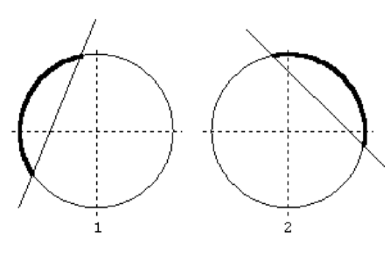
Figure 1: Representation of $S^{1}\times S^{1}$ topology with a threshold $Q\left(x|y\right)$ superimposed.

Each circle in figure 1 represents one of the $S^{1}$ subspaces, so the two circles together represent the product $S^{1}\times S^{1}$. The constraints in equation 31 are represented by each circle being centred on the origin of its subspace ($\left\|\mathbf{x}_{i}\left(\theta_{i}\right)\right\|^{2}$ is constant), and the probability density around each circle being constant ($\left\|\frac{\partial\mathbf{x}_{i}\left(\theta_{i}\right)}{\partial\theta_{i}}\right\|^{2}$ is constant). A single threshold function $Q\left(\mathbf{x|y}\right)$ is represented by a chord cutting through each circle (with 0 and 1 indicating on which side of the chord the threshold is triggered). The $\mathbf{x}_{i}$ that lie above threshold in each subspace are highlighted. Both $\mathbf{x}_{1}$ and $\mathbf{x}_{2}$ must lie above threshold in order to ensure $Q\left(\mathbf{x|y}\right)=1$, i.e. they must both lie within regions that are highlighted in figure 1. In this case node $\mathbf{y}$ will be said to be “attached” to both subspace 1 and subspace 2. A special case arises when the chord in one of the subspaces (say it is $\mathbf{x}_{2}$) does not intersect the circle at all, and the circle lies on the side of the chord where the threshold is triggered. In this case $Q\left(\mathbf{x|y}\right)$ does not depend on $\mathbf{x}_{2}$, so that $\Pr\left(\mathbf{y|x}_{1},\mathbf{x}_{2}\right)=\Pr\left(\mathbf{y|x}_{1}\right)$, in which case node $\mathbf{y}$ will be said to be “attached” to subspace 1 but “detached” from subspace 2. The typical ways in which a node becomes attached to the 2-torus are shown in figure 2.

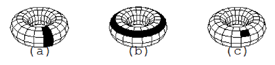
Figure 2: Explicit representation of $S^{1}\times S^{1}$ topology as a torus with the effect of 3 different types of threshold $Q\left(x|y\right)$ shown.

In figure 2(a) the node is attached to one of the $S^{1}$ subspaces and detached from the other. In figure 2(b) the attached and detached subspaces are interchanged with respect to figure 2(a). In figure 2(c) the node is attached to both subspaces.

2.2 All Nodes Attached to One Subspace

Consider the configuration of threshold functions shown in figure 3. This is equivalent to all of the nodes being attached to loops to cover the 2-torus, with a typical node being as shown in figure 2(a) (or, equivalently, figure 2(b)).

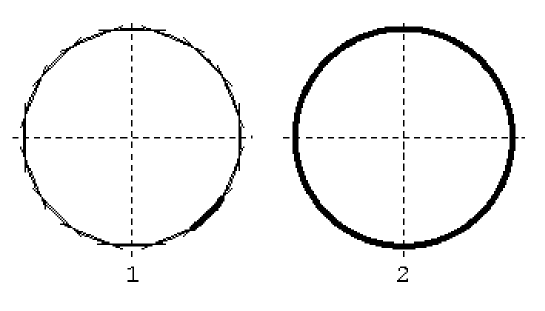
Figure 3: 16 nodes are shown, which are all attached to subspace 1, and all detached from subspace 2.

When $D_{1}+D_{2}$ is minimised, it is assumed that the 4 nodes are symmetrically disposed in subspace 1, as shown. Each is triggered if and only if $\mathbf{x}_{1}$ lies within its quadrant, and one such quadrant is highlighted in figure 3. This implies that only 1 node is triggered at a time. The assumed form of the threshold functions implies $\Pr\left(y\mathbf{|x}_{1},\mathbf{x}_{2}\right)=\Pr\left(y\mathbf{|x}_{1}\right)$, so equation 32 reduces to

$$\begin{array}[]{l}n\int d\mathbf{x}_{1}\,d\mathbf{x}_{2}\Pr\left(\mathbf{x}_{1}|y\right)\Pr\left(\mathbf{x}_{2}\right)\,\left(\mathbf{x}_{1},\mathbf{x}_{2}\right)\\ \\ =\int d\mathbf{x}_{1}\,d\mathbf{x}_{2}\Pr\left(\mathbf{x}_{1}|y\right)\Pr\left(\mathbf{x}_{2}\right)\\ \\ \times\left(\left(n-1\right)\sum_{y^{\prime}=1}^{M}\Pr\left(y^{\prime}\mathbf{|x}_{1}\right)\left(\mathbf{x}_{1}^{\prime}\left(y^{\prime}\right),\mathbf{x}_{2}^{\prime}\left(y^{\prime}\right)\right)+\left(\mathbf{x}_{1}^{\prime}\left(y\right),\mathbf{x}_{2}^{\prime}\left(y\right)\right)\right)\end{array}\ \ \ \$$ (33)

whence

$$\mathbf{x}_{1}^{\prime}\left(y\right) = \int d\mathbf{x}_{1}\Pr\left(\mathbf{x}_{1}|y\right)\,\mathbf{x}_{1}$$

$$\mathbf{x}_{2}^{\prime}\left(y\right) = 0$$ (34)

2.3 All Nodes Attached to Both Subspaces

Consider the configuration of threshold functions shown in figure 4. This is equivalent to all of the nodes being attached to patches to cover the 2-torus, with a typical node being as shown in figure 2(c).

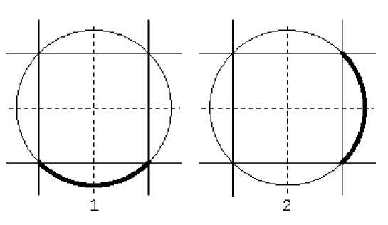
Figure 4: 16 nodes are shown, which are all attached to both subspace 1 and subspace 2.

In this case, when $D_{1}+D_{2}$ is minimised, it is assumed that each subspace is split into 2 halves. This requires a total of 4 nodes, each of which is triggered if, and only if, both $\mathbf{x}_{1}$ and $\mathbf{x}_{2}$ lie on the corresponding half-circles. This implies that only 1 node is triggered at a time. The assumed form of the threshold functions implies that the stationarity condition becomes

$$\begin{array}[]{l}n\,\Pr\left(y\right)\int d\mathbf{x}_{1}\,d\mathbf{x}_{2}\Pr\left(\mathbf{x}_{1},\mathbf{x}_{2}|y\right)\,\left(\mathbf{x}_{1},\mathbf{x}_{2}\right)\\ \\ =\Pr\left(y\right)\int d\mathbf{x}_{1}\,d\mathbf{x}_{2}\Pr\left(\mathbf{x}_{1},\mathbf{x}_{2}|y\right)\\ \\ \times\left(\left(n-1\right)\sum_{y^{\prime}=1}^{M}\Pr\left(y^{\prime}\mathbf{|x}_{1},\mathbf{x}_{2}\right)\left(\mathbf{x}_{1}^{\prime}\left(y^{\prime}\right),\mathbf{x}_{2}^{\prime}\left(y^{\prime}\right)\right)+\left(\mathbf{x}_{1}^{\prime}\left(y\right),\mathbf{x}_{2}^{\prime}\left(y\right)\right)\right)\end{array}\ \ \ \ \$$ (35)

whence

$$\mathbf{x}_{1}^{\prime}\left(y\right) = \int d\mathbf{x}_{1}\Pr\left(\mathbf{x}_{1}|y\right)\mathbf{x}_{1}$$

$$\mathbf{x}_{2}^{\prime}\left(y\right) = \int d\mathbf{x}_{2}\Pr\left(\mathbf{x}_{2}|y\right)\mathbf{x}_{2}$$ (36)

2.4 Half the Nodes Attached to One Subspace, and Half to the Other Subspace

Consider the configuration of threshold functions shown in figure 5. This is equivalent to half of the nodes being attached to loops to cover the 2-torus, with a typical node being as shown in figure 2(a). The other half of the nodes would then be attached in an analogous way, but as shown in figure 2(b). Thus the 2-torus is covered twice over.

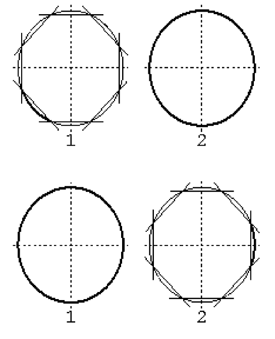
Figure 5: 16 nodes are shown, 8 of which are attached to subspace 1 and detached from subspace 2 (top row), and 8 of which are attached to subspace 2 and detached from subspace 1 (bottom row).

In this case, when $D_{1}+D_{2}$ is minimised, it is assumed that each subspace is split into 2 halves. This requires a total of 4 nodes, each of which is triggered if $\mathbf{x}_{1}$ (or $\mathbf{x}_{2}$) lies on the half-circle in the subspace to which the node is attached. Thus exactly 2 nodes $y_{1}\left(\mathbf{x}_{1}\right)$ and $y_{2}\left(\mathbf{x}_{2}\right)$ are triggered at a time, so that

$$\Pr\left(y|\mathbf{x}_{1},\mathbf{x}_{2}\right) = \frac{1}{2}\left(\delta_{y,y_{1}\left(\mathbf{x}_{1}\right)}+\delta_{y,y_{2}\left(\mathbf{x}_{2}\right)}\right)$$

$$= \frac{1}{2}\left(\Pr\left(y|\mathbf{x}_{1}\right)+\Pr\left(y|\mathbf{x}_{2}\right)\right)$$ (37)

For simplicity, assume that node $y$ is attached to subspace 1, then $\Pr\left(\mathbf{x}_{1},\mathbf{x}_{2}|y\right)=\Pr\left(\mathbf{x}_{1}|y\right)\Pr\left(\mathbf{x}_{2}\right)$ and the stationarity condition becomes

$$\begin{array}[]{l}n\,\Pr\left(y\right)\int d\mathbf{x}_{1}\,d\mathbf{x}_{2}\Pr\left(\mathbf{x}_{1}|y\right)\Pr\left(\mathbf{x}_{2}\right)\,\left(\mathbf{x}_{1},\mathbf{x}_{2}\right)\\ \\ =\Pr\left(y\right)\int d\mathbf{x}_{1}\,d\mathbf{x}_{2}\Pr\left(\mathbf{x}_{1}|y\right)\Pr\left(\mathbf{x}_{2}\right)\\ \\ \times\left(\begin{array}[]{c}\frac{n-1}{2}\sum_{y^{\prime}=1}^{M}\left(\Pr\left(y^{\prime}|\mathbf{x}_{1}\right)+\Pr\left(y^{\prime}|\mathbf{x}_{2}\right)\right)\,\left(\mathbf{x}_{1}^{\prime}\left(y^{\prime}\right),\mathbf{x}_{2}^{\prime}\left(y^{\prime}\right)\right)\\ +\left(\mathbf{x}_{1}^{\prime}\left(y\right),\mathbf{x}_{2}^{\prime}\left(y\right)\right)\end{array}\right)\end{array}\ \ \ \ \ \$$ (38)

This may be simplified to yield

$$\begin{array}[]{l}\ n\int d\mathbf{x}_{1}\Pr\left(\mathbf{x}_{1}|y\right)\,\left(\mathbf{x}_{1},0\right)\\ \\ =\frac{n+1}{2}\left(\mathbf{x}_{1}^{\prime}\left(y\right),\mathbf{x}_{2}^{\prime}\left(y\right)\right)\\ \\ +\frac{n-1}{2}\int d\mathbf{x}_{2}\Pr\left(\mathbf{x}_{2}\right)\sum_{y^{\prime}=1}^{M}\Pr\left(y^{\prime}|\mathbf{x}_{2}\right)\,\left(\mathbf{x}_{1}^{\prime}\left(y^{\prime}\right),\mathbf{x}_{2}^{\prime}\left(y^{\prime}\right)\right)\\ \\ =\frac{n+1}{2}\left(\mathbf{x}_{1}^{\prime}\left(y\right),\mathbf{x}_{2}^{\prime}\left(y\right)\right)+\frac{n-1}{2}\left\langle\mathbf{x}_{1}^{\prime}\left(y\right),\mathbf{x}_{2}^{\prime}\left(y\right)\right\rangle_{2}\end{array}\$$ (39)

Write the 2 subspaces separately (remember that node $y$ is assumed to be attached to subspace 1)

$$\mathbf{x}_{1}^{\prime}\left(y\right) = \frac{2n}{n+1}\int d\mathbf{x}_{1}\Pr\left(\mathbf{x}_{1}|y\right)\mathbf{x}_{1}-\frac{n-1}{n+1}\left\langle\mathbf{x}_{1}^{\prime}\left(y\right)\right\rangle_{2}$$

$$\mathbf{x}_{2}^{\prime}\left(y\right) = -\frac{n-1}{n+1}\left\langle\mathbf{x}_{2}^{\prime}\left(y\right)\right\rangle_{2}$$ (40)

If this result is simultaneously solved with the analogous result for node $y$ attached to subspace 2, then the $\left\langle\cdots\right\rangle$ terms vanish to yield

$$\mathbf{x}_{1}^{\prime}\left(y\right) = \left\{\begin{array}[]{ll}\frac{2n}{n+1}\int d\mathbf{x}_{1}\Pr\left(\mathbf{x}_{1}|y\right)\mathbf{x}_{1}&y\text{ attached to subspace 1}\\ 0&y\text{ attached to subspace 2}\end{array}\right.$$ (43)

$$\mathbf{x}_{2}^{\prime}\left(y\right) = \left\{\begin{array}[]{ll}0&y\text{ attached to subspace 1}\\ \frac{2n}{n+1}\int d\mathbf{x}_{2}\Pr\left(\mathbf{x}_{2}|y\right)\mathbf{x}_{2}&y\text{ attached to subspace 2}\end{array}\right.$$ (46)

2.5 Compare $D_{1}+D_{2}$ for the 3 Different Types of Solution

Consider the left hand side of figure 3 for the case of $M$ nodes, when the $M$ threshold functions form a regular $M$-ogon. $\Pr\left(\mathbf{x|}y\right)$ then denotes the part of the circle that is associated with node $y$, whose radius of gyration squared is given by (assuming that the circle has unit radius)

$$R_{M} \equiv \left\|\int d\mathbf{x}\Pr\left(\mathbf{x|}y\right)\,\mathbf{x}\right\|^{2}$$ (47)

$$= \left(\frac{M}{2\pi}\int_{0}^{\frac{2\pi}{M}}d\theta\cos\theta\right)^{2}$$

$$= \left(\frac{M}{2\pi}\sin\frac{2\pi}{M}\right)^{2}$$

Gather the results for $\left(\mathbf{x}_{1}^{\prime}\left(y\right),\mathbf{x}_{2}^{\prime}\left(y\right)\right)$ in equations 34 (referred to as type 1), 36 (referred to as type 2), and 46 (referred to as type 3) together and insert them into $D_{1}+D_{2}$ in equation 27 to obtain (see appendix E)

$$D_{1}+D_{2}=\left\{\begin{array}[]{ll}\text{constant}-2R_{M}&\text{type 1}\\ \text{constant}-4R_{\sqrt{M}}&\text{type 2}\\ \text{constant}-\frac{4n}{n+1}R_{\frac{M}{2}}&\text{type 3}\end{array}\right.$$ (48)

In figure 6 the 3 solutions are plotted for the case $n=1$.

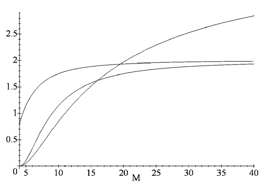
Figure 6: Plots of $-D_{1}-D_{2}$ for $n=1$ for each of the 3 types of optimum.

For $n=1$ the type 3 solution is never optimal, the type 1 solution is optimal for $M\leq 19$, and the type 2 solution is optimal for $M\geq 20.$ This behaviour is intuitively sensible, because a larger number of nodes is required to cover a 2-torus as shown in figure 2(c) than as shown in figure 2(a) (or figure 2(b)).

In figure 7 the 3 solutions are plotted for the case $n=2$.

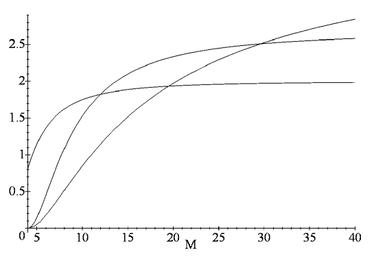
Figure 7: Plots of $-D_{1}-D_{2}$ for $n=2$ for each of the 3 types of optimum.

For $n=2$ the type 1 solution is optimal for $M\leq 12$, and the type 2 solution is optimal for large $M\geq 30$, but there is now an intermediate region $12\leq M\leq 29$ (type 1 and type 3 have an equal $D_{1}+D_{2}$ at $M=12$) where the $n$-dependence of the type 3 solution has now made it optimal. Again, this behaviour is intuitively reasonable, because the type 3 solution requires at least 2 observations in order to be able to yield a small Euclidean resonstruction error in each of the 2 subspaces, i.e. for $n=2$ the 2 nodes that fire must be attached to different subspaces. Note that in the type 3 solution the nodes that fire are not guaranteed to be attached to different subspaces. In the type 3 solution there is a probability $\frac{1}{2^{n}}\frac{n!}{n_{1}!n_{2}!}$ that $n_{i}$ (where $n=n_{1}+n_{2}$) nodes are attached to subspace $i$, so the trend is for the type 3 solution to become more favoured as $n$ is increased.

In figure 8 the 3 solutions are plotted for the case $n\rightarrow\infty$.

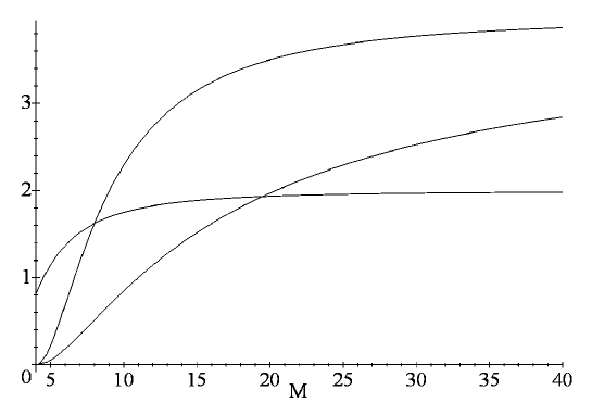
Figure 8: Plots of $-D_{1}-D_{2}$ for $n\rightarrow\infty$ for each of the 3 types of optimum.

For $n\rightarrow\infty\,$ the type 2 solution is never optimal , the type 1 solution is optimal for $M\leq 8$, and the type 3 solution is optimal for $M\geq 8$. The type 2 solution approaches the type 3 solution from below asymptotically as $M\rightarrow\infty$. In figure 9 a phase diagram is given which shows how the relative stability of the 3 types of solution for different $M$ and $n$, where the type 3 solution is seen to be optimal over a large part of the $\left(M,n\right)$ plane.

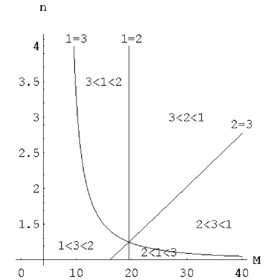
Figure 9: Phase diagram of the regions in which the 3 types of solution are optimal.

Thus the most interesting, and commonly occurring, solution is the one in which half the nodes are attached to one subspace and half to the other subspace (i.e. solution type 3). Although this result has been derived using the non-scaling version of the posterior probability model $\Pr\left(\mathbf{y|x}\right)$ (as in equation 6), it may also be used for scaling posterior probabilities (as given in equation 8) in certain limiting cases, and also for cases where the effect of leakage $\Pr\left(\mathbf{y|y}^{\prime}\right)$ is small.

2.6 Various Extensions

2.6.1 The Effect of Leakage

The effect of leakage will not be analysed in detail here. However, its effect may readily be discussed phenomenologically, because the optimisation acts to minimise the damaging effect of leakage on the posterior probability by ensuring that the properties of nodes that are connected by leakage are similar. This has the most dramatic effect on the type 3 solution, where the way in which the nodes are partitioned into 2 halves must be very carefully chosen in order to minimise the damage due to leakage. If the leakage is presumed to be a local function, so that $\Pr\left(y|y^{\prime}\right)=\pi\left(y-y^{\prime}\right)$, which is a localised “blob”-shaped function, then the properties of adjacent node are similar (after optimisation). Since nodes that are attached to 2 different subspaces necessarily have very different properties, whereas nodes that are attached to the same subspace can have similar properties, it follows that the nodes must split into 2 continguous halves, where nodes $1,2,\cdots,\frac{M}{2}$ are attached to subspace 1 and nodes $\frac{M}{2}+1,\frac{M}{2}+2,\cdots,M$ are attached to subspace 2, or vice versa. The effect of leakage is thereby minimised, with the worst effect occurring at the boundary between the 2 halves of nodes.

2.6.2 Modifying the Posterior Probability to Become Scalable

The above analysis has focussed on the non-scaling version of the posterior probability, in which all $M$ nodes act together as a unit. The more general scaling case where the $M$ nodes are split up by the effect of the neighbourhood function $N\left(y\right)$ will not be analysed in detail, because many of its properties are essentially the same as in the non-scaling case. For simplicity assume that the neighbourhood function $N\left(y\right)$ is a “top-hat” with width $w$ (an odd integer) centred on $y$. Impose periodic boundary conditions so that the inverse neighbourhood function $\tilde{N}\left(y\right)$ is also a top-hat, $\tilde{N}\left(y\right)=N\left(y\right)$. In this case an optimum solution in the non-scaling case (with $M=w$) can be directly related to a corresponding optimum solution in the scaling case by simply repeating the node properties periodically every $w$ nodes. Strictly speaking, higher order periodicities can also occur in the scaling case (and can be favoured under certain conditions), where the period is $\frac{w}{k}$ ($k$ is an integer), but these will not be discussed here.

The effect of the periodic replication of node properties is interesting. The type 3 solution (with leakage and with $M=w)$ splits the nodes into 2 halves, where nodes $1,2,\cdots,\frac{w}{2}$ are attached to subspace 1 and nodes $\frac{w}{2}+1,\frac{w}{2}+2,\cdots,w$ are attached to subspace 2, or vice versa. When this is replicated periodically every $w$ nodes it produces an alternating structure of node properties, where $\frac{w}{2}$ nodes are attached to subspace 1, then the next $\frac{w}{2}$ nodes are attached to subspace 2, and thenthe next $\frac{w}{2}$ nodes are attached to subspace 1, and so on. This behaviour is reminiscent of the so-called “dominance stripes” that are observed in the mammalian visual cortex.

3 Experiment

The purpose of this section is to demonstrate the emergence of the dominance stripes in numerical simulations. The main body of the software is concerned with evaluating the derivatives of $D_{1}+D_{2}$, and the main difficulty is choosing an appropriate form for the leakage (this has not yet been automated).

3.1 The Parameters

The parameters that are required for a simulation are as follows:

1. $\left(m_{1},m_{2}\right)$: size of 2D rectangular array of nodes. $M=m_{1}m_{2}$.

2. $\left(i_{1},i_{2}\right)$: size of 2D rectangular input window for each node (odd integers). Ensure that the input window is not too many input data “correlation areas” in size, otherwise dominance stripes may not emerge. Dominance stripes require that the correlation within an input window are substantially stronger than the correlations between input windows that are attached to different subspaces.

3. $\left(w_{1},w_{2}\right)$: size of 2D rectangular neighbourhood window for each node (odd integers). The neighbourhood function $N\left(y_{1},y_{2}\right)$ is a rectangular top-hat centred on $\left(y_{1},y_{2}\right)$. The size of the neighbourhood window has to lie within a limited range to ensure that dominance stripes are produced. This corresponds to ensuring that $M$ lies in the type 3 region of the phase diagram in figure 9. It is also preferable for the size of the neighbourhood window to be substantially smaller than the input window, otherwise different parts of a neighbourhood window will see different parts of the input data, which will make the network behaviour more difficult to interpret.

4. $\left(l_{1},l_{2}\right)$: size of 2D rectangular leakage window for each node (odd integers). For simplicity the leakage $\Pr\left(\mathbf{y|y}^{\prime}\right)$ is assumed to be given by $\Pr\left(\mathbf{y|y}^{\prime}\right)=\pi\left(\mathbf{y}-\mathbf{y}^{\prime}\right)$, where $\pi\left(\mathbf{y}-\mathbf{y}^{\prime}\right)$ is a “top-hat” function of $\mathbf{y}-\mathbf{y}^{\prime}$ which covers a rectangular region of size $\left(l_{1},l_{2}\right)$ centred on $\mathbf{y}-\mathbf{y}^{\prime}=0$. The size of the leakage window must be large enough to correlate the parameters of adjacent nodes, but not so large that it enforces such strong correlations between the node parameters that it destroys dominance stripes.

5. $\nu$: additive noise level used to corrupt each member of the training set.

6. $\kappa$: wavenumber of sinusoids used in the training set. In describing the training sets the index $y$ will be used to denote position in input space, thus position $y$ in input space lies directly “under” node $y$ of the network. In 1D simulations each training vector is a sinusoid of the form $\sin\left(\kappa y+\phi\right)+r$, where $\phi$ is a random phase angle, and $r$ is a random number sampled uniformly from the interval $\left[-\frac{\nu}{2},\frac{\nu}{2}\right]$ - this generates an $S^{1}$ topology training set (i.e. parameterised by 1 random angle). In 2D simulations each training vector is a sinusoid of the form $\sin\left(\kappa\left(y_{1}\cos\theta+y_{2}\sin\theta\right)+\phi\right)+r$, where the additional angle $\theta$ is a random azimuthal orientation for the sine wave - this generates an $S^{1}\times S^{1}$ topology training set (i.e. parameterised by 2 independent random angles). Note that $\kappa i_{1}$ and $\kappa i_{2}$ must be an integer multiple of $2\pi$ in order to ensure that the probability density around the $S^{1}$ subspace generated by $\phi$ has uniform density (in effect, the $S^{1}$ then becomes a circular Lissajous figure, which therefore has uniform probability density, unlike non-circular Lissajous figures), and thus to ensure that there are no artefacts induced by the periodicity of the training data that might mimic the effect of dominance stripes. If $\kappa i_{1}$ and $\kappa i_{2}$ are much greater than $2\pi$ then it is not necessary to fix them to be integer multiples of $2\pi$ - because the fluctuations in the probability density are then negligible. Note that this restriction on the value of $\kappa$ would not have been necessary had complex exponentials been used rather than sinusoids.

7. $s$: number of subspaces. This fixes the number of statistically independent subspaces in the training set. When $s=1$ the training set is generated exactly as above. When $s=2$ the training set is split up as follows. The 1D case has even $y$ in one subspace, and odd $y$ in the other subspace, thus successive components of each training vector alternate between the 2 subspaces. The 2D case has even $y_{1}+y_{2}$ in one subspace, and odd $y_{1}+y_{2}$ in the other subspace, thus each training vector is split up into a chessboard pattern of interlocking subspaces. This strategy readily generalises for $s\geq 3$, although this is not used here. Within each subspace the training vector is generated as above, and the subspaces are generated so that they are statistically independent.

8. $\varepsilon$: update parameter used in gradient descent. This is used to update parameters thus

   $$\text{parameter}\rightarrow\text{parameter}-\varepsilon\,\frac{\partial\left(D_{1}+D_{2}\right)}{\partial\text{parameter}}$$ (49)

   There are 3 internally generated update parameter, which control the update of the 3 different types of parameter, i.e. the biases, the weights, and the reference vectors. This is necessary because these parameters all have different dimensionalities, and by inspection of equation 49 the dimensionality of an update parameter is the dimensionality of the parameter it updates (squared) divided by the dimensionality of the Euclidean distortion. These 3 internal parameters are automatically adjusted to ensure that the average change in absolute value of each of the 3 types of parameter is equal to $\varepsilon$ times the typical diameter of the region of parameter space populated by the parameters. This adjustment is made anew as each training vector is presented. The size of $\varepsilon$ determines the “memory time” of the node parameters. This memory time determines the effective number of training vectors that the nodes are being optimised against, and thus must be sufficiently long (i.e. $\varepsilon$ sufficiently small) that if $s\geq 2$ it is possible to discern that the subspaces are indeed statistically independent. This is crucially important, for dominance stripes cannot be obtained if the subspaces are not sufficiently statistically independent. So $\varepsilon$ must be small, which unfortunately leads to correspondingly long training times.

3.2 Initialisation

The training set is globally translated and scaled so that the components of all of its training vectors lie in the interval $[-1,+1]$. There are 3 parameter types to initialise. The weights were all initialised to random numbers sampled from a uniform distribution in the interval $\left[-0.1,+0.1\right]$, whereas the biasses and the reference vector components were all initialised to 0. Because the 2D simulations took a very long time to run, they were periodically interrupted and the state of all the variables written to an output file. The simulation could then be continued by reading this output file in again and simply continuing where the simulation left off. Alternatively, some of the variables might have their values changed before continuing. In particular, the random number generator could thus be manipulated to simulate the effect of a finite sized training set (i.e. use the same random number seed at the start of each part of the simulation), or an infinite-sized training set (i.e. use a different random number seed at the start of each part of the simulation). The size of the $\varepsilon$ parameter could also thus be manipulated should a large value be required initially, and reduced to a small value later on, as required in order to guarantee that when $n\geq 2$ the input subspaces are seen to be statistically independent, and dominance stripes may emerge.

3.3 Boundary Conditions

There are many ways to choose the boundary conditions. In the numerical simulations periodic boundary conditions will be avoided, because they can lead to artefacts in which the node parameters become topologically trapped. For instance, in a 2D simulation, periodic boundary conditions imply that the nodes sit on a 2-torus. Leakage implies that the node parameter values are similar for adjacent nodes, which limits the freedom for the parameters to adjust their values on the surface of the 2-torus. For instance, any acceptable set of parameters that sits on the 2-torus can be converted into another acceptable set by mapping the 2-torus to itself, so that each of its $S^{1}$ “coils up” an integer number of times onto itself. Such a multiply wrapped parameter configuration is topologically trapped, and cannot be perturbed to its original form. This problem does not arise with non-periodic boundary conditions.

There are several different problems that arise at the boundaries of the array of nodes:

1. The neighbourhood function $N\left(y_{1},y_{2}\right)$ cannot be assumed to be a rectangular top-hat centred on $\left(y_{1},y_{2}\right)$. Instead, it will simply be truncated so that it does not fall off the edge of array of nodes, i.e. $N\left(y_{1},y_{2}\right)=0$ for those $\left(y_{1},y_{2}\right)$ that lie outside the array.

2. The leakage function $\pi\left(y_{1}-y_{1}^{\prime},y_{2}-y_{2}^{\prime}\right)$ will be similarly truncated. However, in this case $\pi\left(y_{1}-y_{1}^{\prime},y_{2}-y_{2}^{\prime}\right)$ must normalise to unity when summed over $\left(y_{1},y_{2}\right)$, so the effect of the truncation must be compensated by scaling the remaining elements of $\pi\left(y_{1}-y_{1}^{\prime},y_{2}-y_{2}^{\prime}\right)$.

3. The input window for each node implies that the input array must be larger than the node array in order that the input windows never fall off the edge of the input array.

3.4 Presentation of Results

The most important result is the emergence of dominance stripes. For $n=2$ there are thus 2 numbers that need to be displayed for each node: the “degree of attachment” to subspace 1, and similarly for subspace 2. There are many ways to measure degree of attachment, for instance the probability density $\Pr\left(\mathbf{x|y}\right)$ gives a direct measurement of how strongly node $\mathbf{y}$ depends on the input vector $\mathbf{x}$, so its “width” or “volume” in each of the subspaces could be used to measure degree of attachment. However, in the simulations presented here (i.e. sinusoidal training vectors) the degree of attachment is measured as the average of the absolute values of the components of the reference vector in the subspace concerned. This measure tends to zero for complete detachment. For 1D simulations 2 dominance plots can be overlaid to show the dominance of subspaces 1 and 2 for each node. For 2D simulations it is simplest to present only 1 of these plots as a 2D array of grey-scale pixels, where the grey level indicates the dominance of subspace 1 (or, alternatively, subspace 2).

3.5 1D Simulation

The parameter values used were: $\left(m_{1},m_{2}\right)=(1,100)$, $\left(i_{1},i_{2}\right)=\left(1,41\right)$, $\left(w_{1},w_{2}\right)=\left(1,21\right)$, $\left(l_{1},l_{2}\right)=\left(1,15\right)$, $\kappa=0.3$, $\nu=0.1$, $s=2$, $n=400$, $\varepsilon=0.002$. This value of $\kappa$ implies $\frac{\kappa i_{2}}{2\pi}\simeq 1.96$, so $\kappa$ is approximately an integer multiple of $2\pi$, as required for an artefact-free simulation. In figure 10 a plot of the 2 dominance curves obtained after 3200 training updates is shown.

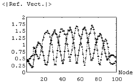
Figure 10: Dominance plots for a 1D simulation with 2 statistically independent training set subspaces.

This dominance plot clearly shows alternating regions where subspace 1 dominates and subspace 2 dominates. The width of the neighbourhood function is 21, which is the same the period of the variations in the dominance plots, i.e. within each set of adjacent 21 nodes half the nodes are attached to subspace 1 and half to subspace 2. There are boundary effects, but these are unimportant.

Appendix A Normalisation of $\Pr\left(\mathbf{y}|\mathbf{x}\right)$

The normalisation of the expression for $\Pr\left(\mathbf{y}|\mathbf{x}\right)$ in equation 8 may be demonstrated as follows:

$$\sum_{\mathbf{y}=\mathbf{1}}^{\mathbf{m}}\Pr\left(\mathbf{y}|\mathbf{x}\right) = \frac{1}{M}\sum_{\mathbf{y}=\mathbf{1}}^{\mathbf{m}}Q\left(\mathbf{x}|\mathbf{y}\right)\sum_{\mathbf{y}^{\prime}\in\tilde{N}\left(\mathbf{y}\right)}\frac{1}{\sum_{\mathbf{y}^{\prime\prime}\in N\left(\mathbf{y}^{\prime}\right)}Q\left(\mathbf{x}|\mathbf{y}^{\prime\prime}\right)}$$ (50)

$$= \frac{1}{M}\sum_{\mathbf{y}^{\prime}=\mathbf{1}}^{\mathbf{m}}\sum_{\mathbf{y}\in N\left(\mathbf{y}^{\prime}\right)}Q\left(\mathbf{x}|\mathbf{y}\right)\frac{1}{\sum_{\mathbf{y}^{\prime\prime}\in N\left(\mathbf{y}^{\prime}\right)}Q\left(\mathbf{x}|\mathbf{y}^{\prime\prime}\right)}$$

$$= \frac{1}{M}\sum_{\mathbf{y}^{\prime}=\mathbf{1}}^{\mathbf{m}}1$$

$$= \frac{m_{1}m_{2}\,\cdots\,m_{d}}{M}$$

$$= 1$$

In the first step the order of the $\mathbf{y}$ and the $\mathbf{y}^{\prime}$ summations is interchanged using $\sum_{\mathbf{y}=\mathbf{1}}^{\mathbf{m}}\sum_{\mathbf{y}^{\prime}\in\tilde{N}\left(\mathbf{y}\right)}\left(\cdots\right)=\sum_{\mathbf{y}^{\prime}=\mathbf{1}}^{\mathbf{m}}\sum_{\mathbf{y}\in N\left(\mathbf{y}^{\prime}\right)}\left(\cdots\right)$, in the second step the numerator and denominator of the summand cancel out.

Appendix B Upper Bound for Multiple Firing Model

It is possible to simplify equation 10 by using the following identity

$$\mathbf{x}-\mathbf{x}^{\prime}\left(\mathbf{y}_{1},\mathbf{y}_{2},\cdots\mathbf{y}_{n}\right)\equiv\frac{1}{n}\sum_{i=1}^{n}\left(\mathbf{x}-\mathbf{x}^{\prime}\left(\mathbf{y}_{i}\right)\right)+\frac{1}{n}\sum_{i=1}^{n}\left(\mathbf{x}^{\prime}\left(\mathbf{y}_{i}\right)-\mathbf{x}^{\prime}\left(\mathbf{y}_{1},\mathbf{y}_{2},\cdots\mathbf{y}_{n}\right)\right)$$ (51)

Note that this holds for all choices of $\mathbf{x}^{\prime}\left(\mathbf{y}_{i}\right)$. This allows the Euclidean distance to be expanded thus

$$\ \ \left\|\mathbf{x}-\mathbf{x}^{\prime}\left(\mathbf{y}_{1},\mathbf{y}_{2},\cdots\mathbf{y}_{n}\right)\right\|^{2}$$

$$= \frac{1}{n^{2}}\sum_{i=1}^{n}\left\|\mathbf{x}-\mathbf{x}^{\prime}\left(\mathbf{y}_{i}\right)\right\|^{2}$$ (55)

$$\ \ \ \ \ +\frac{1}{n^{2}}\sum_{\begin{array}[]{c}i,j=1\\ i\neq j\end{array}}^{n}\left(\mathbf{x}-\mathbf{x}^{\prime}\left(\mathbf{y}_{i}\right)\right)\cdot\left(\mathbf{x}-\mathbf{x}^{\prime}\left(\mathbf{y}_{j}\right)\right)$$

$$\ \ \ \ \ \ -\frac{2}{n^{2}}\sum_{i,j=1}^{n}\left(\mathbf{x}-\mathbf{x}^{\prime}\left(\mathbf{y}_{i}\right)\right)\left(\mathbf{x}^{\prime}\left(\mathbf{y}_{j}\right)-\mathbf{x}^{\prime}\left(\mathbf{y}_{1},\mathbf{y}_{2},\cdots\mathbf{y}_{n}\right)\right)$$

$$\ \ \ \ \ \ +\frac{1}{n^{2}}\left\|\sum_{i=1}^{n}\left(\mathbf{x}^{\prime}\left(\mathbf{y}_{i}\right)-\mathbf{x}^{\prime}\left(\mathbf{y}_{1},\mathbf{y}_{2},\cdots\mathbf{y}_{n}\right)\right)\right\|^{2}$$

Each term of this expansion can be inserted into equation 10 to yield

term 1 $$= \frac{1}{n}\sum_{\mathbf{y}=\mathbf{1}}^{\mathbf{m}}\int d\mathbf{x}\Pr\left(\mathbf{x}\right)\Pr\left(\mathbf{y}|\mathbf{x}\right)\left\|\mathbf{x}-\mathbf{x}^{\prime}\left(\mathbf{y}\right)\right\|^{2}$$

term 2 $$= \frac{n-1}{n}\int d\mathbf{x}\Pr\left(\mathbf{x}\right)\sum_{\mathbf{y}_{1},\mathbf{y}_{2}=\mathbf{1}}^{\mathbf{m}}\Pr\left(\mathbf{y}_{1},\mathbf{y}_{2}|\mathbf{x}\right)\left(\mathbf{x}-\mathbf{x}^{\prime}\left(\mathbf{y}_{1}\right)\right)\left(\mathbf{x}-\mathbf{x}^{\prime}\left(\mathbf{y}_{2}\right)\right)$$

term 3 $$= -2\times\text{term 4}$$

term 4 $$= \sum_{\mathbf{y}_{1},\mathbf{y}_{2},\cdots\mathbf{y}_{n}=\mathbf{1}}^{\mathbf{m}}\Pr\left(\mathbf{y}_{1},\mathbf{y}_{2},\cdots\mathbf{y}_{n}\right)\left\|\begin{array}[]{c}\mathbf{x}^{\prime}\left(\mathbf{y}_{1},\mathbf{y}_{2},\cdots\mathbf{y}_{n}\right)\\ -\frac{1}{n}\sum_{i=1}^{n}\mathbf{x}^{\prime}\left(\mathbf{y}_{i}\right)\end{array}\right\|^{2}$$ (58)

$\Pr\left(\mathbf{y}_{1},\mathbf{y}_{2},\cdots\mathbf{y}_{n}|\mathbf{x}\right)$ has been assumed to be a symmetric function of $\left(\mathbf{y}_{1},\mathbf{y}_{2},\cdots\mathbf{y}_{n}\right)$ in the first two results, and the definition of $\mathbf{x}^{\prime}\left(\mathbf{y}_{1},\mathbf{y}_{2},\cdots\mathbf{y}_{n}\right)$ in equation 11 has been used to obtain the third result. These results allow $D$ in equation 10 to be expanded as $D=D_{1}+D_{2}-D_{3}$, where

$$D_{1} \equiv \frac{2}{n}\sum_{\mathbf{y}=\mathbf{1}}^{\mathbf{m}}\int d\mathbf{x}\Pr\left(\mathbf{x}\right)\Pr\left(\mathbf{y}|\mathbf{x}\right)\left\|\mathbf{x}-\mathbf{x}^{\prime}\left(\mathbf{y}\right)\right\|^{2}$$

$$D_{2} \equiv \frac{2\left(n-1\right)}{n}\int d\mathbf{x}\Pr\left(\mathbf{x}\right)\sum_{\mathbf{y}_{1},\mathbf{y}_{2}=\mathbf{1}}^{\mathbf{m}}\Pr\left(\mathbf{y}_{1},\mathbf{y}_{2}|\mathbf{x}\right)\left(\mathbf{x}-\mathbf{x}^{\prime}\left(\mathbf{y}_{1}\right)\right)\left(\mathbf{x}-\mathbf{x}^{\prime}\left(\mathbf{y}_{2}\right)\right)$$

$$D_{3} \equiv 2\sum_{\mathbf{y}_{1},\mathbf{y}_{2},\cdots\mathbf{y}_{n}=\mathbf{1}}^{\mathbf{m}}\Pr\left(\mathbf{y}_{1},\mathbf{y}_{2},\cdots\mathbf{y}_{n}\right)\left\|\begin{array}[]{c}\mathbf{x}^{\prime}\left(\mathbf{y}_{1},\mathbf{y}_{2},\cdots\mathbf{y}_{n}\right)\\ -\frac{1}{n}\sum_{i=1}^{n}\mathbf{x}^{\prime}\left(\mathbf{y}_{i}\right)\end{array}\right\|^{2}$$ (61)

By noting that $D_{3}\geq 0$, an upper bound for $D$ in the form $D\leq D_{1}+D_{2}$ follows immediately from these results. Note that $D_{1}\geq 0$ whereas $D_{2}$ can have either sign. In the special case where $\Pr\left(\mathbf{y}_{1},\mathbf{y}_{2}|\mathbf{x}\right)=\Pr\left(\mathbf{y}_{1}|\mathbf{x}\right)\Pr\left(\mathbf{y}_{1}|\mathbf{x}\right)$ (i.e. $\mathbf{y}_{1}$ and $\mathbf{y}_{2}$ are independent of each other given that $x$ is known) $D_{2}$ reduces to

$$D_{2}\equiv\frac{2\left(n-1\right)}{n}\int d\mathbf{x}\Pr\left(\mathbf{x}\right)\left\|\sum_{\mathbf{y}=\mathbf{1}}^{\mathbf{m}}\Pr\left(\mathbf{y}|\mathbf{x}\right)\left(\mathbf{x}-\mathbf{x}^{\prime}\left(\mathbf{y}\right)\right)\right\|^{2}$$ (62)

which is manifestly positive. This is the form of $D_{2}$ that is used throughout this paper.

Appendix C Derivatives of the Objective Function

$D_{1}$ and $D_{2}$ are as given in equation 12, i.e. it is assumed that $\Pr\left(\mathbf{y}_{1},\mathbf{y}_{2}|\mathbf{x}\right)=\Pr\left(\mathbf{y}_{2}|\mathbf{x}\right)\Pr\left(\mathbf{y}_{2}|\mathbf{x}\right)$ and $\Pr\left(\mathbf{y}|\mathbf{x}\right)$ has the scalable form given in equation 8. Define a compact matrix notation as follows

$$\ \begin{array}[]{ll}L_{\mathbf{y},\mathbf{y}^{\prime}}\equiv\Pr\left(\mathbf{y^{\prime}|y}\right)&P_{\mathbf{y,y}^{\prime}}\equiv\Pr\left(\mathbf{y^{\prime}|x;y}\right)\\ p_{\mathbf{y}}\equiv\sum_{\mathbf{y}^{\prime}\in\tilde{N}\left(\mathbf{y}\right)}P_{\mathbf{y^{\prime},y}}&\left(L^{T}p\right)_{\mathbf{y}}\equiv\sum_{\mathbf{y}^{\prime}=\mathbf{1}}^{\mathbf{m}}L_{\mathbf{y}^{\prime}\mathbf{,y}}\,p_{\mathbf{y}^{\prime}}\\ \mathbf{d}_{\mathbf{y}}\equiv\mathbf{x}-\mathbf{x}^{\prime}\left(\mathbf{y}\right)&\left(L\,\mathbf{d}\right)_{\mathbf{y}}\equiv\sum_{\mathbf{y}^{\prime}=\mathbf{1}}^{\mathbf{m}}L_{\mathbf{y},\mathbf{y}^{\prime}}\,\mathbf{d}_{\mathbf{y}^{\prime}}\\ \left(P\,L\,\mathbf{d}\right)_{\mathbf{y}}\equiv\sum_{\mathbf{y}^{\prime}\in N\left(\mathbf{y}\right)}P_{\mathbf{y},\mathbf{y}^{\prime}}\left(L\,\mathbf{d}\right)_{\mathbf{y}^{\prime}}&\left(P^{T}P\,L\,\mathbf{d}\right)_{\mathbf{y}}\equiv\sum_{\mathbf{y}^{\prime}\in\tilde{N}\left(\mathbf{y}\right)}P_{\mathbf{y^{\prime},y}}\left(P\,L\,\mathbf{d}\right)_{\mathbf{y}^{\prime}}\\ e_{\mathbf{y}}\equiv\left\|\mathbf{x}-\mathbf{x}^{\prime}\left(\mathbf{y}\right)\right\|^{2}&\left(L\,e\right)_{\mathbf{y}}\equiv\sum_{\mathbf{y}^{\prime}=\mathbf{1}}^{\mathbf{m}}L_{\mathbf{y},\mathbf{y}^{\prime}}\,e_{\mathbf{y}^{\prime}}\\ \left(P\,L\,e\right)_{\mathbf{y}}\equiv\sum_{\mathbf{y}^{\prime}\in N\left(\mathbf{y}\right)}P_{\mathbf{y,y}^{\prime}}\left(L\,e\right)_{\mathbf{y}^{\prime}}&\left(P^{T}P\,L\,e\right)_{\mathbf{y}}\equiv\sum_{\mathbf{y}^{\prime}\in\tilde{N}\left(\mathbf{y}\right)}P_{\mathbf{y^{\prime},y}}\left(P\,L\,e\right)_{\mathbf{y}^{\prime}}\\ \mathbf{\bar{d}\equiv}\sum_{\mathbf{y}=\mathbf{1}}^{\mathbf{m}}\left(L^{T}p\right)_{\mathbf{y}}\mathbf{d}_{\mathbf{y}}&\text{or }\mathbf{\bar{d}\equiv}\sum_{\mathbf{y}=\mathbf{1}}^{\mathbf{m}}\left(P\,L\,\mathbf{d}\right)_{\mathbf{y}}\end{array}$$ (70)

Using this matrix notation, the functions $\mathbf{f}_{1}\left(\mathbf{x},\mathbf{y}\right)$, $\,\mathbf{f}_{2}\left(\mathbf{x},\mathbf{y}\right)$, $g_{1}\left(\mathbf{x},\mathbf{y}\right)$, and $g_{2}\left(\mathbf{x},\mathbf{y}\right)$ may be defined as

$$\mathbf{f}_{1}\left(\mathbf{x},\mathbf{y}\right) \equiv \left(L^{T}p\right)_{\mathbf{y}}\mathbf{d}_{\mathbf{y}}$$ (71)

$$\mathbf{f}_{2}\left(\mathbf{x},\mathbf{y}\right) \equiv \left(L^{T}p\right)_{\mathbf{y}}\mathbf{\bar{d}}$$ (72)

$$g_{1}\left(\mathbf{x},\mathbf{y}\right) \equiv p_{\mathbf{y}}\left(L\,e\right)_{\mathbf{y}}-\left(P^{T}P\,L\,e\right)_{\mathbf{y}}$$ (73)

$$g_{2}\left(\mathbf{x},\mathbf{y}\right) \equiv \left(p_{\mathbf{y}}\left(L\,\mathbf{d}\right)_{\mathbf{y}}-\left(P^{T}P\,L\,\mathbf{d}\right)_{\mathbf{y}}\right)\cdot\mathbf{\bar{d}}$$ (74)

The variation of $\Pr\left(\mathbf{y}|\mathbf{x};\mathbf{y}^{\prime}\right)$ is then given by

$$\delta\Pr\left(\mathbf{y}|\mathbf{x};\mathbf{y}^{\prime}\right) = \Pr\left(\mathbf{y}|\mathbf{x};\mathbf{y}^{\prime}\right)\left(\begin{array}[]{c}\delta\log Q\left(\mathbf{x}|\mathbf{y}\right)\\ -\sum_{\mathbf{y}^{\prime\prime}\in N\left(\mathbf{y}^{\prime}\right)}\Pr\left(\mathbf{y}^{\prime\prime}|\mathbf{x};\mathbf{y}^{\prime}\right)\delta\log Q\left(\mathbf{x}|\mathbf{y}^{\prime\prime}\right)\end{array}\right)$$ (77)

$$= \Pr\left(\mathbf{y}|\mathbf{x};\mathbf{y}^{\prime}\right)\sum_{\mathbf{y}^{\prime\prime}\in N\left(\mathbf{y}^{\prime}\right)}\delta\log Q\left(\mathbf{x}|\mathbf{y}^{\prime\prime}\right)\left(\delta_{\mathbf{y}^{\prime\prime},\mathbf{y}}-\Pr\left(\mathbf{y}^{\prime\prime}|\mathbf{x};\mathbf{y}^{\prime}\right)\right)$$

$$= P_{\mathbf{y}^{\prime},\mathbf{y}}\sum_{\mathbf{y}^{\prime\prime}\in N\left(\mathbf{y}^{\prime}\right)}\delta\log Q\left(\mathbf{x}|\mathbf{y}^{\prime\prime}\right)\left(\delta_{\mathbf{y}^{\prime\prime},\mathbf{y}}-P_{\mathbf{y}^{\prime},\mathbf{y}^{\prime\prime}}\right)$$ (78)

In order to rearrange the expressions to ensure that only a single dummy index is required at every stage of evaluation of the sums it will be necessary to use the result

$$\sum_{\mathbf{y}=\mathbf{1}}^{\mathbf{m}}\sum_{\mathbf{y}^{\prime}\in N\left(\mathbf{y}\right)}=\sum_{\mathbf{y}^{\prime}=\mathbf{1}}^{\mathbf{m}}\sum_{\mathbf{y}\in\tilde{N}\left(\mathbf{y}^{\prime}\right)}$$ (79)

C.1 Calculate $\frac{\partial D_{1}}{\partial\mathbf{x}^{\prime}\left(\mathbf{y}\right)}$.

The derivative is given by

$$\frac{\partial D_{1}}{\partial\mathbf{x}^{\prime}\left(\mathbf{y}\right)}=-\frac{4}{n\,M}\int d\mathbf{x}\Pr\left(\mathbf{x}\right)\sum_{\mathbf{y}^{\prime}=\mathbf{1}}^{\mathbf{m}}\Pr\left(\mathbf{y}|\mathbf{y}^{\prime}\right)\sum_{\mathbf{y}^{\prime\prime}\in\tilde{N}\left(\mathbf{y}^{\prime}\right)}\Pr\left(\mathbf{y}^{\prime}|\mathbf{x};\mathbf{y}^{\prime\prime}\right)\left(\mathbf{x}-\mathbf{x}^{\prime}\left(\mathbf{y}\right)\right)$$ (80)

Use matrix notation to write this as

$$\frac{\partial D_{1}}{\partial\mathbf{x}^{\prime}\left(\mathbf{y}\right)}=-\frac{4}{n\,M}\int d\mathbf{x}\Pr\left(\mathbf{x}\right)\sum_{\mathbf{y}^{\prime}=\mathbf{1}}^{\mathbf{m}}L_{\mathbf{y}^{\prime},\mathbf{y}}\sum_{\mathbf{y}^{\prime\prime}\in\tilde{N}\left(\mathbf{y}^{\prime}\right)}P_{\mathbf{y}^{\prime\prime}\mathbf{,y}^{\prime}}\,\mathbf{d}_{\mathbf{y}}$$ (81)

Finally remove the explicit summations to obtain the required result

$$\frac{\partial D_{1}}{\partial\mathbf{x}^{\prime}\left(\mathbf{y}\right)} = -\frac{4}{n\,M}\int d\mathbf{x}\Pr\left(\mathbf{x}\right)\left(L^{T}p\right)_{\mathbf{y}}\mathbf{d}_{\mathbf{y}}$$ (82)

$$= -\frac{4}{n\,M}\int d\mathbf{x}\Pr\left(\mathbf{x}\right)\,\mathbf{f}_{1}\left(\mathbf{x},\mathbf{y}\right)$$

C.2 Calculate $\frac{\partial D_{2}}{\partial\mathbf{x}^{\prime}\left(\mathbf{y}\right)}.$

The derivative is given by

$$\frac{\partial D_{2}}{\partial\mathbf{x}^{\prime}\left(\mathbf{y}\right)} = -\frac{4\left(n-1\right)}{n\,M^{2}}\int d\mathbf{x}\Pr\left(\mathbf{x}\right)\left(\sum_{\mathbf{y}^{\prime}=\mathbf{1}}^{\mathbf{m}}\Pr\left(\mathbf{y}|\mathbf{y}^{\prime}\right)\sum_{\mathbf{y}^{\prime\prime}\in\tilde{N}\left(\mathbf{y}^{\prime}\right)}\Pr\left(\mathbf{y}^{\prime}|\mathbf{x};\mathbf{y}^{\prime\prime}\right)\right)$$ (83)

$$\ \times\left(\sum_{\mathbf{\bar{y}}=\mathbf{1}}^{\mathbf{m}}\sum_{\mathbf{y}^{\prime}=\mathbf{1}}^{\mathbf{m}}\Pr\left(\mathbf{\bar{y}}|\mathbf{y}^{\prime}\right)\sum_{\mathbf{y}^{\prime\prime}\in\tilde{N}\left(\mathbf{y}^{\prime}\right)}\Pr\left(\mathbf{y}^{\prime}|\mathbf{x};\mathbf{y}^{\prime\prime}\right)\left(\mathbf{x}-\mathbf{x}^{\prime}\left(\mathbf{\bar{y}}\right)\right)\right)$$

Use matrix notation to write this as

$$\frac{\partial D_{2}}{\partial\mathbf{x}^{\prime}\left(\mathbf{y}\right)} = -\frac{4\left(n-1\right)}{n\,M^{2}}\int d\mathbf{x}\Pr\left(\mathbf{x}\right)\left(\sum_{\mathbf{y}^{\prime}=\mathbf{1}}^{\mathbf{m}}L_{\mathbf{y}^{\prime},\mathbf{y}}\sum_{\mathbf{y}^{\prime\prime}\in\tilde{N}\left(\mathbf{y}^{\prime}\right)}P_{\mathbf{y}^{\prime\prime}\mathbf{,y}^{\prime}}\right)$$ (84)

$$\ \times\left(\sum_{\mathbf{\bar{y}}=\mathbf{1}}^{\mathbf{m}}\sum_{\mathbf{y}^{\prime}=\mathbf{1}}^{\mathbf{m}}L_{\mathbf{y}^{\prime},\mathbf{\bar{y}}}\sum_{\mathbf{y}^{\prime\prime}\in\tilde{N}\left(\mathbf{y}^{\prime}\right)}P_{\mathbf{y}^{\prime\prime}\mathbf{,y}^{\prime}}\mathbf{d}_{\mathbf{\bar{y}}}\right)$$

Finally remove the explicit summations to obtain the required result

$$\frac{\partial D_{2}}{\partial\mathbf{x}^{\prime}\left(\mathbf{y}\right)} = -\frac{4\left(n-1\right)}{n\,M^{2}}\int d\mathbf{x}\Pr\left(\mathbf{x}\right)\left(L^{T}p\right)_{\mathbf{y}}\mathbf{\bar{d}}$$

$$= -\frac{4\left(n-1\right)}{n\,M^{2}}\int d\mathbf{x}\Pr\left(\mathbf{x}\right)\,\mathbf{f}_{2}\left(\mathbf{x},\mathbf{y}\right)$$ (85)

C.3 Calculate $\frac{\delta D_{1}}{\delta\log Q\left(\mathbf{x}|\mathbf{y}\right)}$

The differential is given by

$$\delta D_{1}=\frac{2}{n\,M}\sum_{\mathbf{y}=1}^{\mathbf{m}}\int d\mathbf{x}\Pr\left(\mathbf{x}\right)\sum_{\mathbf{y}^{\prime}=\mathbf{1}}^{\mathbf{m}}\Pr\left(\mathbf{y}|\mathbf{y}^{\prime}\right)\sum_{\mathbf{y}^{\prime\prime}\in\tilde{N}\left(\mathbf{y}^{\prime}\right)}\delta\Pr\left(\mathbf{y}^{\prime}|\mathbf{x};\mathbf{y}^{\prime\prime}\right)\left\|\mathbf{x}-\mathbf{x}^{\prime}\left(\mathbf{y}\right)\right\|^{2}$$ (86)

Use matrix notation to write this as

$$\delta D_{1}=\frac{2}{n\,M}\sum_{\mathbf{y}=\mathbf{1}}^{\mathbf{m}}\int d\mathbf{x}\Pr\left(\mathbf{x}\right)\left(\begin{array}[]{c}\sum_{\mathbf{y}^{\prime}=\mathbf{1}}^{\mathbf{m}}L_{\mathbf{y}^{\prime}\mathbf{,y}}\sum_{\mathbf{y}^{\prime\prime}\in\tilde{N}\left(\mathbf{y}^{\prime}\right)}P_{\mathbf{y}^{\prime\prime},\mathbf{y}^{\prime}}\\ \times\sum_{\mathbf{y}^{\prime\prime\prime}\in N\left(\mathbf{y}^{\prime\prime}\right)}\delta\log Q\left(\mathbf{x}|\mathbf{y}^{\prime\prime\prime}\right)\left(\delta_{\mathbf{y}^{\prime\prime\prime},\mathbf{y}^{\prime}}-P_{\mathbf{y}^{\prime\prime},\mathbf{y}^{\prime\prime\prime}}\right)\end{array}\right)e_{\mathbf{y}}$$ (87)

Reorder the summations to obtain

$$\delta D_{1}=\frac{2}{n\,M}\int d\mathbf{x}\Pr\left(\mathbf{x}\right)\left(\begin{array}[]{c}\sum_{\mathbf{y}^{\prime\prime\prime}=\mathbf{1}}^{\mathbf{m}}\delta\log Q\left(\mathbf{x}|\mathbf{y}^{\prime\prime\prime}\right)\sum_{\mathbf{y}^{\prime\prime}\in\tilde{N}\left(\mathbf{y}^{\prime\prime\prime}\right)}\\ \times\left(\begin{array}[]{c}\sum_{\mathbf{y}^{\prime}\in N\left(\mathbf{y}^{\prime\prime}\right)}\delta_{\mathbf{y}^{\prime\prime\prime},\mathbf{y}^{\prime}}P_{\mathbf{y}^{\prime\prime},\mathbf{y}^{\prime}}\\ -P_{\mathbf{y}^{\prime\prime},\mathbf{y}^{\prime\prime\prime}}\sum_{\mathbf{y}^{\prime}\in N\left(\mathbf{y}^{\prime\prime}\right)}P_{\mathbf{y}^{\prime\prime},\mathbf{y}^{\prime}}\end{array}\right)\sum_{\mathbf{y}=1}^{\mathbf{m}}L_{\mathbf{y}^{\prime}\mathbf{,y}}\,e_{\mathbf{y}}\end{array}\right)$$ (88)

Relabel the indices and evaluate the sum over the Kronecker delta to obtain

$$\delta D_{1} = \frac{2}{n\,M}\sum_{\mathbf{y}=\mathbf{1}}^{\mathbf{m}}\int d\mathbf{x}\Pr\left(\mathbf{x}\right)\delta\log Q\left(\mathbf{x}|\mathbf{y}\right)$$ (92)

$$\times\left(\begin{array}[]{c}\left(\sum_{\mathbf{y}^{\prime}\in\tilde{N}\left(\mathbf{y}\right)}P_{\mathbf{y}^{\prime},\mathbf{y}}\right)\left(\sum_{\mathbf{y}^{\prime}=\mathbf{1}}^{\mathbf{m}}L_{\mathbf{y,y}^{\prime}}\,e_{\mathbf{y}^{\prime}}\right)\\ -\left(\sum_{\mathbf{y}^{\prime\prime\prime}\in\tilde{N}\left(\mathbf{y}\right)}P_{\mathbf{y}^{\prime\prime\prime},\mathbf{y}}\sum_{\mathbf{y}^{\prime\prime}\in N\left(\mathbf{y}^{\prime\prime\prime}\right)}P_{\mathbf{y}^{\prime\prime\prime},\mathbf{y}^{\prime\prime}}\sum_{\mathbf{y}^{\prime}=\mathbf{1}}^{\mathbf{m}}L_{\mathbf{y}^{\prime\prime},\mathbf{y}^{\prime}}\,e_{\mathbf{y}^{\prime}}\right)\end{array}\right)$$

Finally remove the explicit summations to obtain the required result

$$\delta D_{1} = \frac{2}{n\,M}\sum_{\mathbf{y}=\mathbf{1}}^{\mathbf{m}}\int d\mathbf{x}\Pr\left(\mathbf{x}\right)\delta\log Q\left(\mathbf{x}|\mathbf{y}\right)\left(p_{\mathbf{y}}\left(L\,e\right)_{\mathbf{y}}-(P^{T}P\,L\,e)_{\mathbf{y}}\right)$$ (93)

$$= \frac{2}{n\,M}\sum_{\mathbf{y}=\mathbf{1}}^{\mathbf{m}}\int d\mathbf{x}\Pr\left(\mathbf{x}\right)g_{1}\left(\mathbf{x},\mathbf{y}\right)\,\delta\log Q\left(\mathbf{x}|\mathbf{y}\right)$$

C.4 Calculate $\frac{\delta D_{2}}{\delta\log Q\left(\mathbf{x}|\mathbf{y}\right)}$

The differential is given by

$$\delta D_{2} = \frac{4\left(n-1\right)}{n\,M^{2}}\int d\mathbf{x}\Pr\left(\mathbf{x}\right)$$ (94)

$$\times\left(\sum_{\mathbf{y}=\mathbf{1}}^{\mathbf{m}}\sum_{\mathbf{y}^{\prime}=\mathbf{1}}^{\mathbf{m}}\Pr\left(\mathbf{y}|\mathbf{y}^{\prime}\right)\sum_{\mathbf{y}^{\prime\prime}\in\tilde{N}\left(\mathbf{y}^{\prime}\right)}\Pr\left(\mathbf{y}^{\prime}|\mathbf{x};\mathbf{y}^{\prime\prime}\right)\left(\mathbf{x}-\mathbf{x}^{\prime}\left(\mathbf{y}\right)\right)\right)$$

$$\ \cdot\left(\sum_{\mathbf{y}=\mathbf{1}}^{\mathbf{m}}\sum_{\mathbf{y}^{\prime}=\mathbf{1}}^{\mathbf{m}}\Pr\left(\mathbf{y}|\mathbf{y}^{\prime}\right)\sum_{\mathbf{y}^{\prime\prime}\in\tilde{N}\left(\mathbf{y}^{\prime}\right)}\delta\Pr\left(\mathbf{y}^{\prime}|\mathbf{x};\mathbf{y}^{\prime\prime}\right)\left(\mathbf{x}-\mathbf{x}^{\prime}\left(\mathbf{y}\right)\right)\right)$$

Use matrix notation to write this as

$$\delta D_{2} = \frac{4\left(n-1\right)}{n\,M^{2}}\int d\mathbf{x}\Pr\left(\mathbf{x}\right)\left(\sum_{\mathbf{y}=\mathbf{1}}^{\mathbf{m}}\sum_{\mathbf{y}^{\prime}=\mathbf{1}}^{\mathbf{m}}L_{\mathbf{y}^{\prime}\mathbf{,y}}\sum_{\mathbf{y}^{\prime\prime}\in\tilde{N}\left(\mathbf{y}^{\prime}\right)}P_{\mathbf{y}^{\prime\prime},\mathbf{y}^{\prime}}\,\mathbf{d}_{\mathbf{y}}\right)$$ (98)

$$\ \cdot\left(\sum_{\mathbf{y}=\mathbf{1}}^{\mathbf{m}}\begin{array}[]{c}\sum_{\mathbf{y}^{\prime}=\mathbf{1}}^{\mathbf{m}}L_{\mathbf{y}^{\prime}\mathbf{,y}}\sum_{\mathbf{y}^{\prime\prime}\in\tilde{N}\left(\mathbf{y}^{\prime}\right)}P_{\mathbf{y}^{\prime\prime},\mathbf{y}^{\prime}}\\ \times\sum_{\mathbf{y}^{\prime\prime\prime}\in N\left(\mathbf{y}^{\prime\prime}\right)}\delta\log Q\left(\mathbf{x}|\mathbf{y}^{\prime\prime\prime}\right)\left(\delta_{\mathbf{y}^{\prime\prime\prime},\mathbf{y}^{\prime}}-P_{\mathbf{y}^{\prime\prime},\mathbf{y}^{\prime\prime\prime}}\right)\end{array}\mathbf{d}_{\mathbf{y}}\right)$$

Reorder the summations to obtain

$$\delta D_{2} = \frac{4\left(n-1\right)}{n\,M^{2}}\int d\mathbf{x}\Pr\left(\mathbf{x}\right)\left(\sum_{\mathbf{y}=\mathbf{1}}^{\mathbf{m}}\sum_{\mathbf{y}^{\prime}=\mathbf{1}}^{\mathbf{m}}L_{\mathbf{y}^{\prime}\mathbf{,y}}\sum_{\mathbf{y}^{\prime\prime}\in\tilde{N}\left(\mathbf{y}^{\prime}\right)}P_{\mathbf{y}^{\prime\prime},\mathbf{y}^{\prime}}\,\mathbf{d}_{\mathbf{y}}\right)$$ (103)

$$\ \cdot\left(\begin{array}[]{c}\sum_{\mathbf{y}^{\prime\prime\prime}=\mathbf{1}}^{\mathbf{m}}\delta\log Q\left(\mathbf{x}|\mathbf{y}^{\prime\prime\prime}\right)\sum_{\mathbf{y}^{\prime\prime}\in\tilde{N}\left(\mathbf{y}^{\prime\prime\prime}\right)}\\ \times\left(\begin{array}[]{c}\sum_{\mathbf{y}^{\prime}\in N\left(\mathbf{y}^{\prime\prime}\right)}\delta_{\mathbf{y}^{\prime\prime\prime},\mathbf{y}^{\prime}}P_{\mathbf{y}^{\prime\prime},\mathbf{y}^{\prime}}\\ -P_{\mathbf{y}^{\prime\prime},\mathbf{y}^{\prime\prime\prime}}\sum_{\mathbf{y}^{\prime}\in N\left(\mathbf{y}^{\prime\prime}\right)}P_{\mathbf{y}^{\prime\prime},\mathbf{y}^{\prime}}\end{array}\right)\sum_{\mathbf{y}=\mathbf{1}}^{\mathbf{m}}L_{\mathbf{y}^{\prime}\mathbf{,y}}\,\mathbf{d}_{\mathbf{y}}\end{array}\right)$$

Relabel the indices and evaluate the sum over the Kronecker delta to obtain

$$\delta D_{2} = \frac{4\left(n-1\right)}{n\,M^{2}}\sum_{\mathbf{y}=\mathbf{1}}^{\mathbf{m}}\int d\mathbf{x}\Pr\left(\mathbf{x}\right)\delta\log Q\left(\mathbf{x}|\mathbf{y}\right)$$ (107)

$$\times\left(\begin{array}[]{c}\left(\sum_{\mathbf{y}^{\prime}\in\tilde{N}\left(\mathbf{y}\right)}P_{\mathbf{y}^{\prime},\mathbf{y}}\right)\left(\sum_{\mathbf{y}^{\prime}=\mathbf{1}}^{\mathbf{m}}L_{\mathbf{y,y}^{\prime}}\,\mathbf{d}_{\mathbf{y}^{\prime}}\right)\\ -\left(\sum_{\mathbf{y}^{\prime\prime\prime}\in\tilde{N}\left(\mathbf{y}\right)}P_{\mathbf{y}^{\prime\prime\prime},\mathbf{y}}\sum_{\mathbf{y}^{\prime\prime}\in N\left(\mathbf{y}^{\prime\prime\prime}\right)}P_{\mathbf{y}^{\prime\prime\prime},\mathbf{y}^{\prime\prime}}\sum_{\mathbf{y}^{\prime}=\mathbf{1}}^{\mathbf{m}}L_{\mathbf{y}^{\prime\prime}\mathbf{,y}^{\prime}}\,\mathbf{d}_{\mathbf{y}^{\prime}}\right)\end{array}\right)$$

$$\cdot\left(\sum_{\mathbf{y}=\mathbf{1}}^{\mathbf{m}}\sum_{\mathbf{y}^{\prime}=\mathbf{1}}^{\mathbf{m}}L_{\mathbf{y}^{\prime}\mathbf{,y}}\sum_{\mathbf{y}^{\prime\prime}\in\tilde{N}\left(\mathbf{y}^{\prime}\right)}P_{\mathbf{y}^{\prime\prime},\mathbf{y}^{\prime}}\,\mathbf{d}_{\mathbf{y}}\right)$$

Finally remove the explicit summations to obtain the required result

$$\delta D_{2} = \frac{4\left(n-1\right)}{n\,M^{2}}\sum_{\mathbf{y}=\mathbf{1}}^{\mathbf{m}}\int d\mathbf{x}\Pr\left(\mathbf{x}\right)\delta\log Q\left(\mathbf{x}|\mathbf{y}\right)$$ (108)

$$\times\left(p_{\mathbf{y}}\left(L\,\mathbf{d}\right)_{\mathbf{y}}-\left(P^{T}P\,L\,\mathbf{d}\right)_{y}\right)\cdot\mathbf{\bar{d}}$$

$$= \frac{4\left(n-1\right)}{n\,M^{2}}\sum_{\mathbf{y}=\mathbf{1}}^{\mathbf{m}}\int d\mathbf{x}\Pr\left(\mathbf{x}\right)g_{2}\left(\mathbf{x},\mathbf{y}\right)\,\delta\log Q\left(\mathbf{x}|\mathbf{y}\right)$$

Appendix D Expression for $D_{1}+D_{2}$ in Terms of $\mathbf{x}^{\prime}\left(c\right)$

From equation 12 $D_{1}+D_{2}$ can be written as

$$D_{1}+D_{2} = \frac{2}{n}\int d\mathbf{x}\Pr\left(\mathbf{x}\right)\sum_{\mathbf{y}=\mathbf{1}}^{\mathbf{m}}\Pr\left(\mathbf{y}|\mathbf{x}\right)\left(\left\|\mathbf{x}^{\prime}\left(\mathbf{y}\right)\right\|^{2}-2\mathbf{x\cdot x}^{\prime}\left(\mathbf{y}\right)\right)$$

$$\ \ \ +\frac{2\left(n-1\right)}{n}\int d\mathbf{x}\Pr\left(\mathbf{x}\right)$$

$$\ \times\left(\begin{array}[]{c}\left\|\sum_{\mathbf{y}=\mathbf{1}}^{\mathbf{m}}\Pr\left(\mathbf{y}|\mathbf{x}\right)\mathbf{x}^{\prime}\left(\mathbf{y}\right)\right\|^{2}\\ -2\left(\sum_{\mathbf{y}=\mathbf{1}}^{\mathbf{m}}\Pr\left(\mathbf{y}|\mathbf{x}\right)\mathbf{x}^{\prime}\left(\mathbf{y}\right)\right)\cdot\left(\sum_{\mathbf{y}=\mathbf{1}}^{\mathbf{m}}\Pr\left(\mathbf{y}|\mathbf{x}\right)\mathbf{x}\right)\end{array}\right)$$

$$\ \ \ +\text{constant}$$

where the constant terms do not depend on $\mathbf{x}^{\prime}\left(\mathbf{y}\right)$. However, from equation 12 the derivative $\frac{\partial\left(D_{1}+D_{2}\right)}{\partial\mathbf{x}^{\prime}\left(\mathbf{y}\right)}$ can be written as

$$\frac{\partial\left(D_{1}+D_{2}\right)}{\partial\mathbf{x}^{\prime}\left(\mathbf{y}\right)} = -\frac{4}{n}\int d\mathbf{x}\Pr\left(\mathbf{x}\right)\Pr\left(\mathbf{y|x}\right)$$ (115)

$$\ \times\left(\begin{array}[]{c}\mathbf{x-x}^{\prime}\left(\mathbf{y}\right)\\ \\ +\left(n-1\right)\sum_{\mathbf{y}^{\prime}=\mathbf{1}}^{\mathbf{m}}\Pr\left(\mathbf{y}^{\prime}\mathbf{|x}\right)\left(\mathbf{x-x}^{\prime}\left(\mathbf{y}^{\prime}\right)\right)\end{array}\right)$$

Using Bayes’ theorem the stationarity condition $\frac{\partial\left(D_{1}+D_{2}\right)}{\partial\mathbf{x}^{\prime}\left(\mathbf{y}\right)}=0$ yields a matrix equation for the $\mathbf{x}^{\prime}\left(\mathbf{y}\right)$

$$n\int d\mathbf{x}\Pr\left(\mathbf{x|y}\right)\,\mathbf{x=}\left(n-1\right)\sum_{\mathbf{y}^{\prime}=\mathbf{1}}^{\mathbf{m}}\left(\int d\mathbf{x}\Pr\left(\mathbf{x}|\mathbf{y}\right)\Pr\left(\mathbf{y}^{\prime}|\mathbf{x}\right)\right)\mathbf{x}^{\prime}\left(\mathbf{y}^{\prime}\right)+\mathbf{x}^{\prime}\left(\mathbf{y}\right)$$ (116)

which may then be used to replace all instances of $\mathbf{x}$ in equation D. This yields the result

$$D_{1}+D_{2} = -\frac{2}{n}\int d\mathbf{x}\Pr\left(\mathbf{x}\right)\sum_{\mathbf{y}=\mathbf{1}}^{\mathbf{m}}\Pr\left(\mathbf{y}|\mathbf{x}\right)\left\|\mathbf{x}^{\prime}\left(\mathbf{y}\right)\right\|^{2}$$

$$\ \ \ -\frac{2\left(n-1\right)}{n}\int d\mathbf{x}\Pr\left(\mathbf{x}\right)\left\|\sum_{\mathbf{y}=\mathbf{1}}^{\mathbf{m}}\Pr\left(\mathbf{y}|\mathbf{x}\right)\mathbf{x}^{\prime}\left(\mathbf{y}\right)\right\|^{2}$$

$$\ \ \ +\text{constant}$$

Appendix E Comparison of $D_{1}+D_{2}$ for Different Types of Optima

In order to compare the value of $D_{1}+D_{2}$ that is obtained when different types of supposedly optimum configurations of the threshold functions $Q\left(\mathbf{x|y}\right)$ are tried, the $\mathbf{x}^{\prime}\left(\mathbf{y}\right)$ that solves $\frac{\partial\left(D_{1}+D_{2}\right)}{\partial\mathbf{x}^{\prime}\left(\mathbf{y}\right)}=0$ (see appendix D) must be inserted into the expression for $D_{1}+D_{2}$. In the following derivations the constant term is omitted, and the definition $R_{M}\equiv\left\|\int d\mathbf{x}\Pr\left(\mathbf{x|}y\right)\,\mathbf{x}\right\|^{2}$ (see equation 47) has been used.

E.1 Type 1 Optimum: all the nodes are attached one subspace

In equation 27 $D_{1}+D_{2}$ becomes

$$D_{1}+D_{2} = -\frac{2}{n}\int d\mathbf{x}\Pr\left(\mathbf{x}\right)\sum_{y=1}^{M}\Pr\left(y|\mathbf{x}\right)\left\|\left(\int d\mathbf{x}_{1}\Pr\left(\mathbf{x}_{1}|y\right)\,\mathbf{x}_{1},0\right)\right\|^{2}$$

$$\ -\frac{2\left(n-1\right)}{n}\int d\mathbf{x}\Pr\left(\mathbf{x}\right)\left\|\sum_{y=1}^{M}\Pr\left(y|\mathbf{x}\right)\left(\int d\mathbf{x}_{1}\Pr\left(\mathbf{x}_{1}|y\right)\,\mathbf{x}_{1},0\right)\right\|^{2}$$

$$= -\frac{2}{n}R_{M}-\frac{2\left(n-1\right)}{n}R_{M}$$

$$= -2R_{M}$$ (118)

E.2 Type 2 Optimum: all the nodes are attached both subspaces

In equation 27 $D_{1}+D_{2}$ becomes

$$D_{1}+D_{2} = -\frac{2}{n}\int d\mathbf{x}\Pr\left(\mathbf{x}\right)\sum_{y=1}^{M}\Pr\left(y|\mathbf{x}\right)$$

$$\ \times\left\|\left(\int d\mathbf{x}_{1}\Pr\left(\mathbf{x}_{1}|y\right)\mathbf{x}_{1},\int d\mathbf{x}_{2}\Pr\left(\mathbf{x}_{2}|y\right)\mathbf{x}_{2}\right)\right\|^{2}$$

$$\ -\frac{2\left(n-1\right)}{n}\int d\mathbf{x}\Pr\left(\mathbf{x}\right)$$

$$\ \times\left\|\sum_{y=1}^{M}\Pr\left(y|\mathbf{x}\right)\left(\int d\mathbf{x}_{1}\Pr\left(\mathbf{x}_{1}|y\right)\mathbf{x}_{1},\int d\mathbf{x}_{2}\Pr\left(\mathbf{x}_{2}|y\right)\mathbf{x}_{2}\right)\right\|^{2}$$

$$= -\left(\frac{2}{n}+\frac{2\left(n-1\right)}{n}\right)2R_{\sqrt{M}}$$

$$= -4R_{\sqrt{M}}$$ (119)

E.3 Type 3 Optimum: half the nodes are attached one subspace and half are attached to the other

In equation 27 $D_{1}+D_{2}$ becomes

$$D_{1}+D_{2} = -\frac{2}{n}\left(\frac{2n}{n+1}\right)^{2}\int d\mathbf{x}\Pr\left(\mathbf{x}\right)$$ (125)

$$\ \times\left(\begin{array}[]{c}\sum_{y=1}^{\frac{M}{2}}\Pr\left(y|\mathbf{x}\right)\left\|\left(\int d\mathbf{x}_{1}\Pr\left(\mathbf{x}_{1}|y\right)\mathbf{x}_{1},0\right)\right\|^{2}\\ +\sum_{y=\frac{M}{2}+1}^{M}\Pr\left(y|\mathbf{x}\right)\left\|\left(0,\int d\mathbf{x}_{2}\Pr\left(\mathbf{x}_{2}|y\right)\mathbf{x}_{2}\right)\right\|^{2}\end{array}\right)$$

$$\ -\frac{2\left(n-1\right)}{n}\left(\frac{2n}{n+1}\right)^{2}\int d\mathbf{x}\Pr\left(\mathbf{x}\right)$$

$$\ \times\left\|\left(\begin{array}[]{c}\sum_{y=1}^{\frac{M}{2}}\Pr\left(y|\mathbf{x}\right)\int d\mathbf{x}_{1}\Pr\left(\mathbf{x}_{1}|y\right)\mathbf{x}_{1},\\ \sum_{y=\frac{M}{2}+1}^{M}\Pr\left(y|\mathbf{x}\right)\int d\mathbf{x}_{2}\Pr\left(\mathbf{x}_{2}|y\right)\mathbf{x}_{2}\end{array}\right)\right\|^{2}$$

$$= -\left(\frac{2n}{n+1}\right)^{2}\left(2\frac{1}{2}\frac{2}{n}+2\left(\frac{1}{2}\right)^{2}\frac{2\left(n-1\right)}{n}\right)R_{\frac{M}{2}}$$

$$= -\frac{4n}{n+1}R_{\frac{M}{2}}$$ (126)

References

- [1] Luttrell S P, 1994, A Bayesian analysis of self-organising maps, Neural Computation, 6, 767-794.
- [2] Luttrell S P, 1994, Partitioned mixture distribution: an adaptive Bayesian network for low-level image processing, IEE Proc. Vision Image Signal Processing, 141, 251-260.