Systems with large flexible server pools: Instability of “natural” load balancing

Abstract

We consider general large-scale service systems with multiple customer classes and multiple server (agent) pools, mean service times depend both on the customer class and server pool. It is assumed that the allowed activities (routing choices) form a tree (in the graph with vertices being both customer classes and server pools). We study the behavior of the system under a natural (load balancing) routing/scheduling rule, Longest-Queue Freest-Server (LQFS-LB), in the many-server asymptotic regime, such that the exogenous arrival rates of the customer classes, as well as the number of agents in each pool, grow to infinity in proportion to some scaling parameter $r$. Equilibrium point of the system under LQBS-LB is the desired operating point, with server pool loads minimized and perfectly balanced.

Our main results are as follows. (a) We show that, quite surprisingly (given the tree assumption), for certain parameter ranges, the fluid limit of the system may be unstable in the vicinity of the equilibrium point; such instability may occur if the activity graph is not “too small.” (b) Using (a), we demonstrate that the sequence of stationary distributions of diffusion-scaled processes [measuring $O(\sqrt{r})$ deviations from the equilibrium point] may be nontight, and in fact may escape to infinity. (c) In one special case of interest, however, we show that the sequence of stationary distributions of diffusion-scaled processes is tight, and the limit of stationary distributions is the stationary distribution of the limiting diffusion process.

and

t1Supported by the NSF Graduate Research Fellowship.

1 Introduction

Large-scale service systems (such as call centers) with heterogeneous customer and server (agent) populations bring up the need for efficient dynamic control policies that match arriving (or waiting) customers and available servers. In this setting, two goals are desirable. On the one hand, customers should not be kept waiting, if this is possible. On the other hand, idle time should be distributed fairly among the servers. For example, one would like to avoid the situation in which one of the server pools is fully busy while another one has significant numbers of idle agents.

Consider a general system, where the arrival rate of class $i$ customers is $\Lambda_{i}$, the service rate of a class $i$ customer by type $j$ agent is $\mu_{ij}$, and the server pool sizes are $B_{j}$. Another very desirable feature of a dynamic control is insensitivity to parameters $\Lambda_{i}$ and $\mu_{ij}$. That is, the assignment of customers to server pools should, to the maximal degree possible, depend only on the current system state, and not on prior knowledge of arrival rates or mean service times, because those parameters may not be known in advance and, moreover, they may be changing in time.

If the system objective is to minimize the maximum average load of any server pool, a “static” optimal control can be obtained by solving a linear program, called static planning problem (SPP), which has $B_{j}$’s, $\mu_{ij}$’s and $\Lambda_{i}$’s as parameters. An optimal solution to the SPP will prescribe optimal average rates $\Lambda_{ij}$ at which arriving customers should be routed to the server pools. Typically (in a certain sense) the solution to SPP is unique and the basic activities, that is, routing choices $(ij)$ for which $\Lambda_{ij}>0$, form a tree; let us assume this is the case. It is possible to design a dynamic control policy, which achieves the load balancing objective without a priori knowledge of input rates $\Lambda_{i}$—the Shadow Routing policy in StolyarTezcanunderload , StolyarTezcan does just that, and in the process it “automatically identifies” the basic activity tree. Shadow Routing policy, however, does need to “know” the service rates $\mu_{ij}$.

The key question we address in this paper is as follows. Suppose a control policy does not know the service rates $\mu_{ij}$, but “somehow” it does know the structure of the basic activity tree, and restrict routing to this tree only. [E.g., all feasible activities, i.e., those $(ij)$’s for which $\mu_{ij}>0$, may form a tree simply by the structure of the system. Another example: if Shadow Routing has some estimates of $\mu_{ij}$, this will not be sufficient for it to identify the optimal routing rates, but may very well be sufficient to correctly identify the basic activity tree.] What is an efficient load balancing policy in this case?

If routing is restricted to a tree, it is very natural to conjecture that simple policies of the type considered by Gurvich and Whitt GurvichWhitt , Atar, Shaki and Shwartz Atar2009 and Armony and Ward ArmonyWard , which are of the “serve longest queue” and “join least loaded pool” type, should “typically be good enough.” Some of the results in these (and other) papers, in fact, prove optimal behavior of simple load balancing schemes on a finite time interval; which further supports the above informal conjecture. One of the main contributions of our work is to show that, surprisingly, the above conjecture is not correct for a general parameter setting. The key reason is that a “natural” load balancing, even if it is done along an a priori given optimal tree, may render the system unstable in the vicinity of equilibrium point.

The specific control rule we analyze in this paper can be seen as a special case of the Queue-and-Idleness Ratio rule considered in GurvichWhitt . Within the given (basic) activity tree, if an arriving customer sees multiple available servers, it will choose the server pool with the smallest load; while if a server sees several customers waiting in queues, it will take a customer from the longest queue. We call this rule Longest-Queue Freest-Server (LQFS-LB).

We consider a many-server asymptotic regime, such that $\Lambda_{i}=\lambda_{i}r$ [or sometimes $\Lambda_{i}=\lambda_{i}r+O(\sqrt{r})$], $B_{j}=\beta_{j}r$, where $\lambda_{i}$ and $\beta_{j}$ are some positive constants, $r\to\infty$ is a scaling parameter and $\mu_{ij}$ remain constant. Our key results show that the fluid limit of the system process (obtained via space-scaling by $1/r$) can be unstable in the vicinity of the equilibrium point. This is very counterintuitive, because it would be reasonable to expect the contrary: that a simple load balancing in a system with activity graph free of cycles would be “well behaved.”

Using the fluid limit local instability (when such occurs), we prove that the sequence of stationary distributions of diffusion-scaled processes [measuring $O(\sqrt{r})$ deviations from the equilibrium point] may be nontight, and in fact may escape to infinity. This of course means, in particular, that the behavior of the diffusion limit in the vicinity of equilibrium point on a finite time interval, may not be relevant to the system behavior in steady state, because the system “does not spend any time” in the $O(\sqrt{r})$-vicinity of the equilibrium point.

In addition to the instability examples, we prove that in several cases the fluid limit will be (at least locally) stable. We demonstrate that fluid limit of any underloaded system with at most two customer classes, or critically loaded system with at most four customer classes, is always locally stable. We also demonstrate local stability in the case when the service rate depends only on the customer type (but not server pool, as long as it can serve it). In the case when the service rate depends only on the server type (but not customer type, as long as it can be served), we show more—the global stability of the fluid limit.

General results on the asymptotics of stationary distributions (most importantly—their tightness), especially in the many-server systems’ diffusion limit, are notoriously difficult to derive; for recent results in this direction see GamarnikZeevi , GamarnikMomcilovic . In the special case when the service rate depends only on the server type, we prove that under the LQFS-LB policy the sequence of stationary distributions of diffusion-scaled processes is tight, and the limit of stationary distributions is the stationary distribution of the limiting diffusion process.

The structure of the paper is as follows. In Section 2 we present the model, define the static planning problem and related notions and define the LQFS-LB policy. In Section 3 we define fluid models of the system, derive their basic properties in the vicinity of an equilibrium point, and define local stability. Section 4 contains fluid model stability results in the two special cases when the service rate depends on server class only or on customer type only. Our key results on local instability of fluid models are presented in Section 5. In Section 6 we consider an underloaded system (with optimal average utilization being $1-\varepsilon<1$), and prove possible evanescence of stationary distributions of the diffusion scaled processes. Finally, Section 7 considers the so-called Halfin–Whitt asymptotic regime [where the optimal average utilization is $1-O(1/\sqrt{r})$], and contains two main results on the asymptotics of stationary distributions of the diffusion scaled processes: (a) possible evanescence under certain parameters and (b) tightness (and “limit interchange”) result for the case when the service rate depends only on the server type.

2 Model

2.1 The model; static planning (LP) problem

Consider the model in which there are $I$ customer classes, or types, labeled $1,2,\ldots,I$, and $J$ server (agent) pools, or classes, labeled $1,2,\ldots,J$ (generally, we will use the subscripts $i$, $i^{\prime}$ for customer classes, and $j$, $j^{\prime}$ for server pools). The sets of customer classes and server classes will be denoted by ${\mathcal{I}}$ and ${\mathcal{J}}$, respectively.

We are interested in the scaling properties of the system as it grows large. The meaning of “grows large” is as follows. We consider a sequence of systems indexed by a scaling parameter $r$. As $r$ grows, the arrival rates and the sizes of the service pools, but not the speed of service, increase. Specifically, in the $r$th system, customers of type $i$ enter the system as a Poisson process of rate $\lambda^{r}_{i}=r\lambda_{i}+o(r)$, while the $j$th server pool has $r\beta_{j}$ individual servers. (All $\lambda_{i}$ and $\beta_{j}$ are positive parameters.) Customers may be accepted for service immediately upon arrival, or enter a queue; there is a separate queue for each customer type. Customers do not abandon the system. When a customer of type $i$ is accepted for service by a server in pool $j$, the service time is exponential of rate $\mu_{ij}$; the service rate depends both on the customer type and the server type, but not on the scaling parameter $r$. If customers of type $i$ cannot be served by servers of class $j$, the service rate is $\mu_{ij}=0$.

We would like to balance the proportion of busy servers across the server pools, while keeping the system operating efficiently. Let $\lambda_{ij}^{r}$ be the average rates at which type $i$ customers are routed to server pools $j$. We would like the system state to be such that $\lambda^{r}_{ij}$ are close to $\lambda_{ij}r$, where $\{\lambda_{ij}\}$ is an optimal solution to the following static planning problem (SPP), which is the following linear program:

$$\min_{\lambda_{ij},\rho}\rho,$$ (1)

subject to

$$\lambda_{ij} \geq 0\qquad\forall i,j,$$ (2)

$$\sum_{j}\lambda_{ij} = \lambda_{i}\qquad\forall i,$$ (3)

$$\sum_{i}\lambda_{ij}\big{/}(\beta_{j}\mu_{ij}) \leq \rho\qquad\forall j.$$ (4)

We assume that the SPP has a unique optimal solution $\{\lambda_{ij},i\in{\mathcal{I}},j\in{\mathcal{J}}\},\rho$; and it is such that the basic activities, that is, those pairs, or edges, $(ij)$ for which $\lambda_{ij}>0$, form a (connected) tree in the graph with vertices set ${\mathcal{I}}\cup{\mathcal{J}}$. The set of basic activities is denoted ${\mathcal{E}}$. These assumptions constitute the complete resource pooling (CRP) condition, which holds “generically;” see StolyarTezcan , Theorem 2.2. For a customer type $i$, let ${\mathcal{S}}(i)=\{j\dvtx(ij)\in{\mathcal{E}}\}$; for a server type $j$, let ${\mathcal{C}}(j)=\{i\dvtx(ij)\in{\mathcal{E}}\}$.

Note that under the CRP condition, all (“server pool capacity”) constraints (4) are binding; in other words, the optimal solution to SPP minimizes and “perfectly balances” server pool loads. Optimal dual variables $\nu_{i},i\in{\mathcal{I}}$ and $\alpha_{j},j\in{\mathcal{J}}$, corresponding to constraints (3) and (4), respectively, are unique and all strictly positive; $\nu_{i}$ is interpreted as the “workload” associated with one type $i$ customer, and $\alpha_{j}$ is interpreted as the (scaled by $1/r$) maximum rate at which server pool $j$ can process workload. The following relations hold:

$$\alpha_{j} = \max_{i}\nu_{i}\beta_{j}\mu_{ij},\qquad\nu_{i}=\min_{j}\alpha_{j}/(\beta_{j}\mu_{ij}),$$

$$\sum_{j}\alpha_{j} = 1,\qquad\sum_{i}\lambda_{i}\nu_{i}=\rho\sum_{j}\alpha_{j}=\rho.$$

If $\rho<1$, the system is called underloaded; if $\rho=1$, the system is called critically loaded. In this paper we consider both cases.

In this paper, we assume that the basic activity tree is known in advance, and restrict our attention to the basic activities only. Namely, we assume that a type $i$ customer service in pool $j$ is allowed only if $(ij)\in{\mathcal{E}}$. [Equivalently, we can a priori assume that ${\mathcal{E}}$ is the set of all possible activities, i.e., $\mu_{ij}=0$ when $(ij)\notin{\mathcal{E}}$, and ${\mathcal{E}}$ is a tree. In this case CRP requires that all feasible activities are basic.]

Let $\psi_{ij}^{*}=\lambda_{ij}/\mu_{ij}$. Continuing our interpretation of the optimal operating point of the system, let $\Psi^{r}_{ij}(t)$ be the number of servers of type $j$ serving customers of type $i$ at time $t$. It is desirable to have $\Psi^{r}_{ij}(t)=r\psi^{*}_{ij}+o(r)$. Later on we will be also interested in the question of whether or not the $o(r)$ term can in fact be $O(\sqrt{r})$.

2.2 Longest-Queue, Freest-Server load balancing algorithm (LQFS-LB)

For the rest of the paper, we analyze the performance of the following intuitive load balancing algorithm.

We introduce the following notation (for the system with scaling parameter $r$):

$\Psi^{r}_{ij}(t)$ the number of servers of type $j$ serving customers of type $i$ at time $t$;

$\Psi^{r}_{j}(t)=\sum_{i}\Psi^{r}_{ij}(t)$ the total number of busy servers of type $j$ at time $t$;

$\Psi^{r}_{i}(t)=\sum_{j}\Psi^{r}_{ij}(t)$ the total number of servers serving type $i$ customers at time $t$;

$\Xi^{r}_{j}(t)=\Psi^{r}_{j}(t)/\beta_{j}$ the instantaneous load of server pool $j$ at time $t$;

$Q^{r}_{i}(t)$ the number of customers of type $i$ waiting for service at time $t$;

$X^{r}_{i}(t)=\Psi^{r}_{i}(t)+Q^{r}_{i}(t)$ the total number of customers of type $i$ in the system at time $t$.

The algorithm consists of two parts: routing and scheduling. “Routing” determines where an arriving customer goes if it sees available servers of several different types. “Scheduling” determines which waiting customer a server picks if it sees customers of several different types waiting in queue.

Routing: If an arriving customer of type $i$ sees any unoccupied servers in server classes in ${\mathcal{S}}(i)$, it will pick a server in the least loaded server pool, that is, $j\in\arg\min_{j\in{\mathcal{S}}(i)}\Xi^{r}_{j}(t)$. (Ties are broken in an arbitrary Markovian manner.)

Scheduling: If a server of type $j$, upon completing a service, sees a customer of a class in ${\mathcal{C}}(j)$ in queue, it will pick the customer from the longest queue, that is, $i\in\arg\max_{j\in{\mathcal{C}}(j)}Q^{r}_{i}$. (Ties are broken in an arbitrary Markovian manner.)

By GurvichWhitt , Remark 2.3, the LQFS-LB algorithm described here is a special case of the algorithm proposed by Gurvich and Whitt, with constant probabilities $p_{i}=\frac{1}{I}$ (queues “should” be equal), $v_{j}=\frac{\beta_{j}}{\sum\beta_{j}}$ (the proportion of idle servers “should” be the same in all server pools).

2.3 Basic notation

Vector $(\xi_{i},i\in{\mathcal{I}})$, where $\xi$ can be any symbol, is often written as $(\xi_{i})$ or $\xi_{{\mathcal{I}}}$; similarly, $(\xi_{j},i\in{\mathcal{J}})=(\xi_{j})=\xi_{{\mathcal{J}}}$ and $(\xi_{ij},(ij)\in{\mathcal{E}})=(\xi_{ij})=\xi_{{\mathcal{E}}}$. We will treat $(\xi_{ij})=\xi_{{\mathcal{E}}}$ as a vector, even though its elements have two indices. Unless specified otherwise, $\sum_{i}\xi_{ij}=\sum_{i\in{\mathcal{C}}(j)}\xi_{ij}$ and $\sum_{j}\xi_{ij}=\sum_{j\in{\mathcal{S}}(i)}\xi_{ij}$. For functions (or random processes) $(\xi(t),t\geq 0)$ we often write $\xi(\cdot)$. (And similarly for functions with domain different from $[0,\infty)$.) So, for example, $(\xi_{i}(\cdot))$ and $\xi_{{\mathcal{I}}}(\cdot)$ both signify $((\xi_{i}(t),i\in{\mathcal{I}}),t\geq 0)$. The indicator function of a set $A$ is denoted ${\mathbf{1}}_{A}$; that is, ${\mathbf{1}}_{A}(\omega)=1$ if $\omega\in A$ and 0 otherwise.

The symbol $\Longrightarrow$ denotes convergence in distribution of either random variables in the Euclidean space $\mathbb{R}^{d}$ (with appropriate dimension $d$), or random processes in the Skorohod space $D^{d}[\eta,\infty)$ of RCLL (right-continuous with left limits) functions on $[\eta,\infty)$, for some constant $\eta\geq 0$. (Unless explicitly specified otherwise, $\eta=0$.) The symbol $\stackrel{{\scriptstyle w}}{{\rightarrow}}$ denotes the weak convergence of probability measures on ${\mathbb{R}}^{d}$, or its one-point compactification $\overline{{\mathbb{R}}}{}^{d}={\mathbb{R}}^{d}\cup\{*\}$, where $*$ is the “point at infinity.” We always consider the Borel $\sigma$-algebras on ${\mathbb{R}}^{d}$ and $\overline{{\mathbb{R}}}{}^{d}$.

Standard Euclidean norm of a vector $x\in\mathbb{R}^{d}$ is denoted $|x|$. The symbol $\to$ denotes ordinary convergence in ${\mathbb{R}}^{d}$ or $\overline{{\mathbb{R}}}{}^{d}$. Abbreviation u.o.c. means uniform on compact sets convergence of functions, with the argument (usually in $[0,\infty)$) which is clear from the context; w.p.1 means convergence with probability 1; $\dot{f}(t)$ means $(d/dt)f(t)$. Transposition of a matrix $H$ is denoted $H^{\dagger}$; in matrix expressions vectors are understood as column-vectors.

3 Fluid model

3.1 Definition

We now consider the behavior of fluid models associated with this system. A fluid model is a set of trajectories that w.p.1 contains any limit of fluid-scaled trajectories of the original stochastic system. (We postpone proving this relationship between the fluid models and fluid limits until Section 3.4, in order to not interrupt the main content of Section 3; for now, we just formally define fluid models.)

The term fluid model denotes a set of Lipschitz continuous functions

$$\bigl{\{}\bigl{(}a_{i}(\cdot)\bigr{)},\bigl{(}x_{i}(\cdot)\bigr{)},\bigl{(}q_{i}(\cdot)\bigr{)},\bigl{(}\psi_{ij}(\cdot)\bigr{)},\bigl{(}\rho_{j}(\cdot)\bigr{)}\bigr{\}},$$

which satisfy the equations below. [Here $a_{i}(\cdot)=(a_{i}(t),t\geq 0)$, and similarly for other components.] The last two equations involving derivatives are to be satisfied at all regular points $t$, when the derivatives in question exist. The interpretation of the components is as follows: $a_{i}(t)$ is the total number (actually, “amount,” i.e., the number, scaled by $1/r$) of arrivals of type $i$ customers into the system by time $t$, $x_{i}(t)$ is the number (“amount”) of customers of type $i$ in the system at time $t$, $q_{i}(t)$ is the number (“amount”) of customers of type $i$ waiting in queue at time $t$, $\psi_{ij}(t)$ is the number (“amount”) of customers of type $i$ being served by servers of type $j$ at time $t$, and $\rho_{j}(t)$ is the instantaneous load [proportion of busy servers, the limit of $\Xi^{r}_{j}(t)/r$] in server pool $j$.

$$a_{i}(t) = \lambda_{i}t\qquad\forall i\in{\mathcal{I}},$$ (5a)

$$x_{i}(t) = q_{i}(t)+\sum_{j}\psi_{ij}(t)\qquad\forall i\in{\mathcal{I}},$$ (5b)

$$x_{i}(t) = x_{i}(0)+a_{i}(t)-\sum_{j}\int_{0}^{t}\mu_{ij}\psi_{ij}(s)\,ds\qquad\forall i\in{\mathcal{I}},$$ (5c)

$$\rho_{j}(t) = \frac{1}{\beta_{j}}\sum_{i}\psi_{ij}(t)\qquad\forall j\in{\mathcal{J}},$$ (5d)

$$\rho_{j}(t) = 1\mbox{ if $q_{i}(t)>0$ for any $i\in{\mathcal{C}}(j)$}\qquad\forall j\in{\mathcal{J}}.$$ (5e)

For any set of server types ${\mathcal{J}}^{*}\subseteq{\mathcal{J}}$ and any set of customer types ${\mathcal{I}}^{*}\subseteq{\mathcal{I}}$ such that $q_{i}(t)>0$ for all $i\in{\mathcal{I}}^{*}$, and $q_{i}(t)>q_{i^{\prime}}(t)$ whenever $i\in{\mathcal{I}}^{*}$, $i^{\prime}\notin{\mathcal{I}}^{*}$ and ${\mathcal{S}}(i)\cap{\mathcal{S}}(i^{\prime})\cap{\mathcal{J}}^{*}\neq\varnothing$,

$$\sum_{i\in{\mathcal{I}}^{*}}\sum_{j\in{\mathcal{S}}(i)\cap{\mathcal{J}}^{*}}\dot{\psi}_{ij}(t)$$

$$\qquad=\sum_{j\in\bigcup_{i\in{\mathcal{I}}^{*}}{\mathcal{S}}(i)\cap{\mathcal{J}}^{*}}\sum_{i^{\prime}\in{\mathcal{C}}(j)}\mu_{i^{\prime}j}\psi_{i^{\prime}j}(t)-\sum_{i\in{\mathcal{I}}^{*}}\sum_{j\in{\mathcal{S}}(i)\cap{\mathcal{J}}^{*}}\mu_{ij}\psi_{ij}(t).$$

For any sets of customer types ${\mathcal{I}}_{*}\subseteq{\mathcal{I}}$, and any set of server types ${\mathcal{J}}_{*}\subseteq{\mathcal{J}}$ such that $\rho_{j}(t)<1$ for all $j\in{\mathcal{J}}_{*}$, and $\rho_{j}(t)<\rho_{j^{\prime}}(t)$ whenever $j\in{\mathcal{J}}_{*}$, $j^{\prime}\notin{\mathcal{J}}_{*}$, and ${\mathcal{C}}(j)\cap{\mathcal{C}}(j^{\prime})\cap{\mathcal{I}}_{*}\neq\varnothing$,

$$\qquad\sum_{j\in{\mathcal{J}}_{*}}\sum_{i\in{\mathcal{C}}(j)\cap{\mathcal{I}}_{*}}\dot{\psi}_{ij}(t)=\sum_{i\in\bigcup_{j\in{\mathcal{J}}_{*}}{\mathcal{C}}(j)\cap{\mathcal{I}}_{*}}\lambda_{i}-\sum_{j\in{\mathcal{J}}_{*}}\sum_{i\in{\mathcal{C}}(j)\cap{\mathcal{I}}_{*}}\mu_{ij}\psi_{ij}(t).$$ (5fb)

The meaning of (3.1) is as follows. Consider a set of server types ${\mathcal{J}}^{*}$. If a set of customer types ${\mathcal{I}}^{*}$ consists of the “longest queues for ${\mathcal{J}}^{*}$” (we will make this more precise), then servers in pools $j^{*}\in{\mathcal{J}}^{*}$, whenever they finish serving some customer, will immediately replace her with someone from a queue in ${\mathcal{I}}^{*}$. In this case, the total number of customers of types ${\mathcal{I}}^{*}$ in service by servers of types ${\mathcal{J}}^{*}$ will be increasing at the total rate of servicing all customers by servers in ${\mathcal{J}}^{*}$, less the rate of servicing customers of types ${\mathcal{I}}^{*}$ by servers in ${\mathcal{J}}^{*}$. The requirements that ${\mathcal{I}}^{*}$ needs to satisfy for this to be the case are, that there be no customer types outside ${\mathcal{I}}^{*}$ with longer queues that servers in ${\mathcal{J}}^{*}$ can serve. For example, a one-element set ${\mathcal{I}}^{*}=\{i^{*}\}$ is a valid choice for a one-element set ${\mathcal{J}}^{*}=\{j^{*}\}$ if and only if the customer type $i^{*}\in{\mathcal{C}}(j^{*})$ has the (strictly) longest queue among all of the customer types that can be served by $j^{*}$.

The second equation, (5fb), describes the fact that if a set of server pools ${\mathcal{J}}_{*}$ consists of the “least loaded server pools available to ${\mathcal{I}}_{*}$,” then servers in pools $j^{*}\in{\mathcal{J}}^{*}$, whenever they finish serving some customer, will immediately replace her with someone from queue $i^{*}$. For example, a one-element set ${\mathcal{J}}_{*}=\{j_{*}\}$ is a valid choice for a one-element set ${\mathcal{I}}_{*}=\{i_{*}\}$ if and only if the server pool $j_{*}\in{\mathcal{S}}(i_{*})$ has the (strictly) smallest load $\rho_{j_{*}}$ among all of the server pools that can serve $i_{*}$.

3.2 Behavior in the vicinity of equilibrium point

We define the equilibrium (invariant) point of the underloaded ($\rho<1$) fluid model to be the state $\psi_{ij}=\psi^{*}_{ij}$ and $q_{i}=q=0$ for all $i\in{\mathcal{I}}$, $j\in{\mathcal{J}}$. [All other components of the fluid model are also constant and uniquely defined by $(\psi^{*}_{ij})$ and $q$.] Clearly, $\psi_{ij}(t)\equiv\psi^{*}_{ij}$ and $q_{i}(t)\equiv q$ is indeed a stationary fluid model. Desirable system behavior would be to have $(\psi_{ij}(t))\to(\psi^{*}_{ij})$ as $t\to\infty$.

Note that if the initial system state is in the vicinity of the equilibrium point (with $\rho<1$), then there is no queueing in the system, and we can describe the system with just the variables $(\psi_{ij}(t))$. This will be true for at least some time (depending on $\rho$ and the initial distance to the equilibrium point), because the fluid model is Lipschitz.

The following is a “state space collapse” result for the underloaded fluid model in the neighborhood of the equilibrium point.

Theorem 3.1

Let $\rho<1$. There exists a sufficiently small $\varepsilon>0$, depending only on the system parameters, such that for all sufficiently small $\delta$ the following holds. There exist $T_{1}=T_{1}(\delta)$ and $T_{2}=T_{2}(\delta)$, $0<T_{1}<T_{2}$, such that if the initial system state $(\psi_{ij}(0))$ satisfies

$$\bigl{|}\bigl{(}\psi_{ij}(0)\bigr{)}-\bigl{(}\psi^{*}_{ij}\bigr{)}\bigr{|}<\delta,$$

then for all $t\in[T_{1},T_{2}]$ the system state satisfies

$$\bigl{|}\bigl{(}\psi_{ij}(t)\bigr{)}-\bigl{(}\psi^{*}_{ij}\bigr{)}\bigr{|}<\varepsilon,\qquad\rho_{j}(t)=\rho_{j^{\prime}}(t)\qquad\mbox{for all $j,j^{\prime}\in{\mathcal{J}}$}.$$

Moreover, $T_{1}\downarrow 0$ and $T_{2}\uparrow\infty$ as $\delta\downarrow 0$. The evolution of the system on $[T_{1},T_{2}]$ is described by a linear ODE, specified below by (9).

If the fluid system is critically loaded ($\rho=1$), it may have queues at equilibrium, and the equilibrium is nonunique. Namely, the definition of an equilibrium (invariant) point for $\rho=1$ is the same as for the underloaded system, except the condition on the queues becomes $q_{i}=q$ for some constant $q\geq 0$. In the next Theorem 3.2 we will only consider the case of positive queues ($q>0$) for the critically loaded fluid model.

Theorem 3.2

Let $\rho=1$, and consider an equilibrium point with $q>0$. There exists a sufficiently small $\varepsilon>0$, depending only on the system parameters, such that for all sufficiently small $\delta>0$ the following holds. There exist $T_{1}=T_{1}(\delta)$ and $T_{2}=T_{2}(\delta)$, $0<T_{1}<T_{2}$, such that if the initial system state satisfies

$$\bigl{|}\bigl{(}\psi_{ij}(0)\bigr{)}-\bigl{(}\psi^{*}_{ij}\bigr{)}\bigr{|}<\delta,\qquad\bigl{|}q_{i}(0)-q\bigr{|}<\delta\qquad\mbox{for all $i\in{\mathcal{I}}$},$$

then for all $t\in[T_{1},T_{2}]$ the system state satisfies

$$\bigl{|}\bigl{(}\psi_{ij}(t)\bigr{)}-\bigl{(}\psi^{*}_{ij}\bigr{)}\bigr{|} < \varepsilon,\qquad\bigl{|}q_{i}(t)-q\bigr{|}<\varepsilon\qquad\mbox{for all $i\in{\mathcal{I}}$},$$

$$q_{i}(t) = q_{i^{\prime}}(t)\qquad\mbox{for all $i,i^{\prime}\in{\mathcal{I}}$}.$$

Moreover, $T_{1}\downarrow 0$ and $T_{2}\uparrow\infty$ as $\delta\downarrow 0$. The evolution of the system on $[T_{1},T_{2}]$ is described by a linear ODE specified below by (10).

In the rest of this section and the paper, the values associated with a stationary fluid model, “sitting” at an equilibrium point, are referred to as nominal. For example, $\psi_{ij}^{*}$ is the nominal occupancy (of pool $j$ by type $i$), $\lambda_{i}$ is the nominal arrival rate, $\lambda_{ij}$ is the nominal routing rate [along activity $(ij)$], $\psi^{*}_{ij}\mu_{ij}=\lambda_{ij}$ is the nominal service rate (of type $i$ in pool $j$), $\sum_{j}\psi^{*}_{ij}\mu_{ij}=\lambda_{i}$ is the nominal total service rate (of type $i$), $\rho$ is the nominal total occupancy (of each pool $j$), etc. Proof of Theorem 3.1 Let us choose a suitably small $\varepsilon>0$ (we will specify how small later). Because the fluid model trajectories are continuous, we can always choose some $T_{2}>0$ such that, for all sufficiently small $\delta>0$, if $|(\psi_{ij}(0))-(\psi^{*}_{ij})|<\delta$, then $|(\psi_{ij}(t))-(\psi^{*}_{ij})|<\varepsilon$ for all $t\leq T_{2}$. We will show that $\rho_{j}(t)=\rho_{j^{\prime}}(t)$ for all $j,j^{\prime}\in{\mathcal{J}}$, in $[T_{1},T_{2}]$ for some $T_{1}$ depending on $\delta$.

Consider $\rho_{*}(t)=\min_{j}\rho_{j}(t)$, $\rho^{*}(t)=\max_{j}\rho_{j}(t)$ and assume $\rho_{*}(t)<\rho^{*}(t)$. Let ${\mathcal{J}}_{*}(t)=\{j\dvtx\rho_{j}(t)=\rho_{*}(t)\}$. As long as $\rho_{*}(t)<\rho^{*}(t)$, ${\mathcal{J}}_{*}(t)$ is of course a strict subset of ${\mathcal{J}}$. The total arrival rate to servers of type $j\in{\mathcal{J}}_{*}(t)$ is $\sum_{i\in\bigcup_{j\in{\mathcal{J}}_{*}(t)}{\mathcal{C}}(j)}\lambda_{i}$. By the assumption of the connectedness of the basic activity tree, this is strictly greater (by a constant) than the nominal arrival rate $\sum_{i\in{\mathcal{C}}(j),j\in{\mathcal{J}}_{*}(t)}\lambda_{ij}$. The total rate of departures from those servers is $\sum_{i\in{\mathcal{C}}(j),j\in{\mathcal{J}}_{*}(t)}\mu_{ij}\psi_{ij}(t)$. For small $\varepsilon$, the assumption $|(\psi_{ij}(t))-(\psi^{*}_{ij})|<\varepsilon$ implies that this is close to the nominal departure rate, so the arrival rate exceeds the service rate by at least a constant. (This determines what “suitably small” means for $\varepsilon$ in terms of the system parameters.) Consequently, as long as $\rho_{*}(t)<\rho^{*}(t)$, the minimal load $\rho_{*}(t)$ is increasing at a rate bounded below by a constant. Similarly, as long as $\rho_{*}(t)<\rho^{*}(t)$, the maximal load $\rho^{*}(t)$ is decreasing at a rate bounded below by a constant. Therefore, the difference $\rho^{*}(t)-\rho_{*}(t)$ is decreasing at a rate bounded below by a constant whenever it is positive. Thus, in finite time $T_{1}=T_{1}(\delta)$ we will arrive at a state $\rho_{*}(t)=\rho^{*}(t)$. [Clearly, $T_{1}(\delta)\to 0$ as $\delta\to 0$.] Since the function $\rho^{*}(\cdot)-\rho_{*}(\cdot)$ is Lipschitz (hence absolutely continuous), bounded below by 0 and (for $t\leq T_{2}$) has nonpositive derivative whenever it is differentiable, the condition $\rho_{*}(t)=\rho^{*}(t)$ will continue to hold for $T_{1}\leq t\leq T_{2}$.

It remains to derive the differential equation, and to show that $T_{2}$ can be chosen depending on $\delta$ so that $T_{2}\uparrow\infty$ as $\delta\downarrow 0$.

Once we are confined to the manifold $\rho_{j}(t)=\rho_{j^{\prime}}(t)=\rho(t)$ for all $t$, the system evolution is determined in terms of only $I$ independent variables. Decreasing $\varepsilon$ if necessary to ensure that there is no queueing while $|(\psi_{ij}(t))-(\psi^{*}_{ij})|<\varepsilon$, we can take the $I$ variables to be $\psi_{i}(t):=\sum_{j}\psi_{ij}(t)$. Given $(\psi_{i}(t))$ we know $\rho(t)$ as $(\sum_{i}\psi_{i}(t))/(\sum_{j}\beta_{j})$. Consequently, we know $\sum_{i}\psi_{ij}(t)=\rho(t)\beta_{j}$ and $\sum_{j}\psi_{ij}(t)=\psi_{i}(t)$. On a tree, this allows us to solve for $\psi_{ij}(t)$; the relationship will clearly be linear, that is,

$$\bigl{(}\psi_{ij}(t)\bigr{)}=M\bigl{(}\psi_{i}(t)\bigr{)}$$ (6)

for some matrix $M$. For future reference, we define the (“load balancing”) linear mapping $M$ from $y\in{\mathbb{R}}^{I}$ to $z=(z_{ij},(ij)\in{\mathcal{E}})\in{\mathbb{R}}^{I+J-1}$ as follows: $z=My$ is the unique solution of

$$\eta=\frac{\sum_{i}y_{i}}{\sum_{j}\beta_{j}};\qquad\sum_{i}z_{ij}=\eta\beta_{j}\qquad\forall j;\qquad\sum_{j}z_{ij}=y_{i}\qquad\forall i.$$ (7)

The evolution of $\psi_{i}(t)$ is given by

$$\dot{\psi}_{i}(t)=\lambda_{i}-\sum_{j}\mu_{ij}\psi_{ij}(t)\qquad\forall i.$$ (8)

[This follows from (5c) and the fact that $q_{i}(t)=0$.] Then, by the above arguments we see that this entails (in matrix form)

$$\bigl{(}\dot{\psi}_{i}(t)\bigr{)}=(\lambda_{i})+A_{u}\bigl{(}\psi_{i}(t)\bigr{)},$$ (9)

where $A_{u}$ is an $I\times I$ matrix, $A_{u}=GM$. Here, $G$ is a $I\times(I+J-1)$ matrix with entries $G_{i,(kj)}=-\mu_{ij}$ if $i=k$, and $G_{i,(kj)}=0$ otherwise.

It remains to justify the claim that $T_{2}(\delta)\uparrow\infty$ as $\delta\downarrow 0$. This follows from the fact that, as long as $t\geq T_{1}$ and $|(\psi_{ij}(t))-(\psi^{*}_{ij})|<\varepsilon$, the evolution of the system is described by the linear ODE above. The solutions have the general form

$$\psi_{\mathcal{I}}(t)-\psi^{*}_{\mathcal{I}} = \exp\bigl{(}A_{u}(t-T_{1})\bigr{)}\bigl{(}\psi_{\mathcal{I}}(T_{1})-\psi^{*}_{\mathcal{I}}\bigr{)},$$

$$\psi_{\mathcal{E}}(t)-\psi^{*}_{\mathcal{E}} = M\bigl{(}\psi_{\mathcal{I}}(t)-\psi^{*}_{\mathcal{I}}\bigr{)},$$

where $M$ and $A_{u}$ are constant matrices depending on the system parameters. Therefore, if $|\psi_{\mathcal{I}}(T_{1})-\psi^{*}_{\mathcal{I}}|\leq\delta$ is sufficiently small, then the time it takes for $\psi_{\mathcal{E}}(t)$ to escape the set $|\psi_{\mathcal{E}}(t)-\psi^{*}_{\mathcal{E}}|<\varepsilon$ can be made arbitrarily large. Since as $\delta\downarrow 0$ we have $T_{1}(\delta)\downarrow 0$, and the system trajectory is Lipschitz, taking $|\psi_{\mathcal{E}}(0)-\psi^{*}_{\mathcal{E}}|<\delta$ for small enough $\delta$ will guarantee that $|\psi_{\mathcal{I}}(T_{1})-\psi^{*}_{\mathcal{I}}|$ is small, and hence we can choose $T_{2}(\delta)\uparrow\infty$.

The proof of Theorem 3.2 proceeds similarly; we outline only the differences. Proof of Theorem 3.2 First, since we assume that $\varepsilon>0$ is sufficiently small and $|q_{i}(t)-q|<\varepsilon$, $i\in{\mathcal{I}}$, for all $t\leq T_{2}$, we clearly have $\rho_{j}(t)=1$, $j\in{\mathcal{J}}$, for all $t\leq T_{2}$. The equality of queue lengths in $[T_{1},T_{2}]$ is shown analogously to the proof of $\rho_{*}(t)=\rho^{*}(t)$ for in the underloaded case. Namely, the smallest queue must increase and the largest queue must decrease [as long as not all $q_{i}(t)$ are equal], because it is getting less (resp., more) service than nominal [we choose $\varepsilon$ small enough for this to be true provided $|(\psi_{ij}(t))-(\psi^{*}_{ij})|<\varepsilon$]. Thus, in $[T_{1},T_{2}]$ we will have $q_{i}(t)=q_{i^{\prime}}(t)$ for all $i,i^{\prime}\in{\mathcal{I}}$.

The linear equation is modified as follows. We have

$$\dot{x}_{i}(t)=\lambda_{i}-\sum_{j}\mu_{ij}\psi_{ij}(t),$$

where $x_{i}(t)=\psi_{i}(t)+q_{i}(t)$. Since we know that all $q_{i}(t)$ are equal and positive, we have $q_{i}(t)=q(t)=\frac{1}{I}(\sum x_{k}(t)-\sum\beta_{j})$, and therefore

$$\dot{\psi}_{i}(t)=\dot{x}_{i}(t)-\frac{1}{I}\sum_{k}\dot{x}_{k}(t).$$

The rest of the arguments proceed as above to give

$$\bigl{(}\dot{\psi}_{i}(t)\bigr{)}=\biggl{(}\lambda_{i}-\frac{1}{I}\sum_{i}\lambda_{i}\biggr{)}+A_{c}\bigl{(}\psi_{i}(t)\bigr{)}$$ (10)

for the appropriate matrix $A_{c}$ which can be computed explicitly from the basic activity tree. (Of course, in $[T_{1},T_{2}]$, the trajectory $(\psi_{ij}(\cdot))$ uniquely determines $(\psi_{i}(\cdot))$, $(x_{i}(\cdot))$ and $(q_{i}(\cdot))$.)

Just as above, the existence of the linear ODE, together with the fact that $T_{1}\downarrow 0$ as $\delta\downarrow 0$, implies that $T_{2}\uparrow\infty$ as $\delta\downarrow 0$.

To compute the matrix $M$, and therefore the matrices $A_{u}$ and $A_{c}$, we will find the following observation useful. If $(\psi_{ij}(t))=M(\psi_{i}(t))$, then the common value $\rho(t)=\rho_{j}(t),\forall j$, is

$$\rho(t)=\sum_{i}\psi_{i}(t)\Big{/}\sum_{j}\beta_{j}.$$

This allows us to find the values $(\psi_{ij}(t))$ from $(\psi_{i}(t))$ as follows: if $i$ is a customer-type leaf, then $\psi_{ij}(t)=\psi_{i}(t)$; if $j$ is a server-type leaf, then $\psi_{ij}(t)=\rho(t)\beta_{j}$; we now remove the leaf and continue with the smaller tree. Inductively, for an activity $i_{0}j_{0}$ we find

$$\quad\psi_{i_{0}j_{0}}(t) = \sum_{i\preceq(i_{0},j_{0})}\psi_{i}(t)-\sum_{j\preceq(i_{0},j_{0})}\rho(t)\beta_{j}$$

$$= \frac{1}{\sum\beta_{j}}\biggl{(}\sum_{i\preceq(i_{0},j_{0})}\sum_{j\preceq(j_{0},i_{0})}\psi_{i}(t)\beta_{j}-\sum_{i\preceq(j_{0},i_{0})}\sum_{j\preceq(i_{0},j_{0})}\psi_{i}(t)\beta_{j}\biggr{)}.$$

Here, the relation $\preceq$ is defined as follows. Suppose we disconnect the basic activity tree by removing the edge $(i_{0},j_{0})$. Then for any node $k$ (either customer type or server type), we say $k\preceq(i_{0},j_{0})$ if it falls in the same component as $i_{0}$; otherwise, $k\preceq(j_{0},i_{0})$.

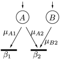
Figure 1: Example for calculation of the matrix $M$.

For example, consider the network in Figure 1. For it, we obtain

$$\pmatrix{\psi_{A1}\cr\psi_{A2}\cr\psi_{B2}}=\pmatrix{\displaystyle\frac{\beta_{1}}{\beta_{1}+\beta_{2}}&\displaystyle\frac{\beta_{1}}{\beta_{1}+\beta_{2}}\vspace*{2pt}\cr\displaystyle 1-\frac{\beta_{1}}{\beta_{1}+\beta_{2}}&\displaystyle-\frac{\beta_{1}}{\beta_{1}+\beta_{2}}\vspace*{2pt}\cr 0&1}\pmatrix{\psi_{A}\cr\psi_{B}}.$$

Since in the underload we have

$$\dot{\psi}_{i}(t)=\lambda_{i}-\sum_{j}\mu_{ij}\psi_{ij}(t),$$

we obtain an expression for $A_{u}$, given in Lemma 3.3(i) just below.

Lemma 3.3

(i) The entries $(A_{u})_{ii^{\prime}}$ of the matrix $A_{u}$ (for the underload case, $\rho<1$) are as follows. The coefficient of $\psi_{i}$ in $\dot{\psi}_{i}$ is

$$(A_{u})_{ii}=-\frac{1}{\sum_{j}\beta_{j}}\sum_{j\in{\mathcal{S}}(i)}\mu_{ij}\sum_{j^{\prime}\preceq(j,i)}\beta_{j^{\prime}}.$$

The coefficient of $\psi_{i^{\prime}}$ in $\dot{\psi}_{i}$ is

$$(A_{u})_{ii^{\prime}} = \frac{1}{\sum_{j}\beta_{j}}\biggl{[}-\sum_{j\in{\mathcal{S}}(i),j\neq j_{ii^{\prime}}}\mu_{ij}\sum_{j^{\prime}\preceq(j,i)}\beta_{j^{\prime}}+\mu_{ij_{ii^{\prime}}}\sum_{j^{\prime}\preceq(i,j_{ii^{\prime}})}\beta_{j^{\prime}}\biggr{]}$$

$$= (A_{u})_{ii}+\mu_{ij_{ii^{\prime}}}.$$

Here, $j_{ii^{\prime}}\in{\mathcal{S}}(i)$ is the neighbor of $i$ such that, after removing the edge $(i,j_{ii^{\prime}})$ from the basic activity tree, nodes $i$ and $i^{\prime}$ will be in different connected components. (Such a node is unique, since there is a unique path along the tree from $i$ to $i^{\prime}$.)

i(ii) The matrix $A_{u}$ is nonsingular.

(iii) The matrix $A_{u}$ depends only on $(\beta_{j})$, $(\mu_{ij})$ and the basic activity tree structure ${\mathcal{E}}$, and does not depend on $(\lambda_{i})$ and $(\psi^{*}_{ij})$.

(i) In the proof of Theorem 3.1 we showed $A_{u}=GM$, where $G$ is a $I\times(I+J-1)$ matrix with entries $G_{i,(kj)}=-\delta_{ik}\mu_{ij}$, where $\delta_{ik}$ is the Kronecker’s delta function and $M$ is the $I\times(I+J-1)$ load-balancing matrix whose entries are determined from the expression (3.2). The form of the entries for $A_{u}$ now follows. The equality between the two expressions for the off-diagonal entries is a consequence of the fact that, for all $j^{\prime}$, exactly one of $j^{\prime}\preceq(ij)$, $j^{\prime}\preceq(ji)$ holds.

(ii) In the case $\rho<1$, in the vicinity of the equilibrium point, the derivative $(\dot{\psi}_{i})=(\lambda_{i})+A_{u}(\psi_{i})$ (which can be any real-valued $I$-dimensional vector, within a small neighborhood of the origin) uniquely determines $(\psi_{ij})$, and then $(\psi_{i})$ as well. Indeed, we have the system of $I+J$ linear equations $\lambda_{i}-\sum_{j}\mu_{ij}\psi_{ij}=\dot{\psi}_{i},\forall i$ and $\sum_{i}\psi_{ij}=\hat{\rho}\beta_{j},\forall j$, for the $I+J$ variables $\hat{\rho},(\psi_{ij})$. This system has unique solution, because $\hat{\rho}$ is uniquely determined by the workload derivative condition

$$\sum_{i}\nu_{i}\dot{\psi}_{i}=\sum_{i}\nu_{i}\lambda_{i}-\sum_{j}\hat{\rho}\alpha_{j},$$

and then the values of $\psi_{ij}$ are determined by sequentially “eliminating” leaves of the basic activity tree.

(iii) Follows from (i).

Lemma 3.4

(i) The entries $(A_{c})_{ii^{\prime}}$ of the matrix $A_{c}$ (for the critical load case, $\rho=1$) are as follows:

$$(A_{c})_{ii^{\prime}}=(A_{u})_{ii^{\prime}}-\frac{1}{I}\sum_{k}(A_{u})_{ki^{\prime}}.$$ (12)

i(ii) The matrix $A_{c}$ has rank $I-1$. The $(I-1)$-dimensional subspace $L=\{y|\sum_{i}y_{i}=0\}$ is invariant under the transformation $A_{c}$, that is, $A_{c}L\subseteq L$. Letting $\pi$ denote the matrix of the orthogonal projection [along $(1,\ldots,1)^{\dagger}$] onto $L$, we have $A_{c}=\pi A_{u}$. Restricted to $L$, the transformation $A_{c}$ is invertible.

(iii) The linear transformation $A_{c}$, restricted to subspace $L$, depends only on $(\mu_{ij})$ and the basic activity tree structure ${\mathcal{E}}$, and does not depend on $(\beta_{j})$, $(\lambda_{i})$ and $(\psi^{*}_{ij})$.

(i) The fluid model here is such that there are always nonzero queues, which are equal across customer types. We can write

$$\dot{\psi}_{i}(t) = \dot{x}_{i}(t)-\frac{1}{I}\sum_{k}\dot{x}_{k}(t)$$

$$= \biggl{(}\lambda_{i}-\sum_{j}\mu_{ij}\psi_{ij}(t)\biggr{)}-\frac{1}{I}\sum_{k}\biggl{(}\lambda_{k}-\sum_{j}\mu_{kj}\psi_{kj}(t)\biggr{)},$$

which implies (12).

i(ii) First of all, it is not surprising that $A_{c}$ does not have full rank: the linear ODE defining $A_{c}$ is such that $\sum_{i}\psi_{i}(t)=\sum_{j}\beta_{j}$ at all times, so there are at most $(I-1)$ degrees of freedom in the system. Also, it will be readily seen that (12) asserts precisely that $A_{c}=\pi A_{u}$. Since $A_{u}$ is invertible and $\pi$ has rank $I-1$, their composition has rank $I-1$. Since the image of $A_{c}$ is contained in $L$, the image of $A_{c}$ (as a map from ${\mathbb{R}}^{I}$) must be equal to all of $L$.

It remains to check that $A_{c}$ restricted to $L$ still has rank $I-1$. To see this, we observe that the simple eigenvalue $0$ of $A_{c}$ has as its unique right eigenvector the vector $A_{u}^{-1}(1,1,\ldots,1)^{\dagger}$. We will be done once we show that this eigenvector does not belong to $L$. Suppose instead that $A_{u}v=(1,1,\ldots,1)^{\dagger}$ for some $v\in L$, $\sum_{i}v_{i}=0$. Then, for a small $\varepsilon>0$, the state $\psi^{*}_{\mathcal{I}}-\varepsilon v$ (with balanced pool loads, all equal to the optimal $\rho$) would be such that the derivatives of all components $\psi_{i}$ would be strictly negative. This is, however, impossible because the total rate at which the system workload is served must be zero,

$$\frac{d}{dt}\sum_{i}\nu_{i}\psi_{i}=\sum_{i}\nu_{i}\lambda_{i}-\sum_{j}\rho\alpha_{j}=0.$$

(iii) The specific expression (12) for $A_{c}$ may depend on the pool sizes $(\beta_{j})$. However, $A_{c}$ is a singular $I\times I$ matrix, and our claim is only about the transformation of the $(I-1)$-dimensional subspace $L$ that $A_{c}$ induces; this transformation does not depend on $(\beta_{j})$, as the following argument shows.

Pick any $(ij)\in{\mathcal{E}}$. Modify the original system by replacing $\beta_{j}$ by $\beta_{j}+\delta$ and $\lambda_{i}$ by $\lambda_{i}+\delta\mu_{ij}$; this means that the nominal $\psi^{*}_{ij}$ is replaced by $\psi^{*}_{ij}+\delta$. Then, using notation $\gamma_{i}(t)=\psi_{i}(t)-\psi^{*}_{i}$, the linear ODE

$$\bigl{(}\dot{\gamma}_{i}(t)\bigr{)}=A\bigl{(}\gamma_{i}(t)\bigr{)},$$ (14)

which we obtain from the ODE (3.2) for the original and modified systems, has exactly the same matrix $A$, which implies $A=A_{c}$. Thus, the transformation $A_{c}$ must not depend on $\beta_{j}$.

An alternative argument is purely analytic. Recall that to compute $(A_{u})_{ij}$ we used (3.2). In critical load, we have $\rho(t)\equiv 1$, so the (left) equation (3.2) for $\psi_{i_{0}j_{0}}(t)$ simplifies to

$$\psi_{i_{0}j_{0}}(t)=\sum_{i\preceq(i_{0},j_{0})}\psi_{i}(t)-\sum_{j\preceq(i_{0},j_{0})}\beta_{j}.$$ (15)

If we substitute this in the right-hand side of (3.2), we will obtain a different expression for $\dot{\psi}_{i}(t)$. While its constant term will depend on $\beta_{\mathcal{J}}$, the linear term will not, since the linear term of (15) does not depend on $\beta_{\mathcal{J}}$. That is, we have found a way of writing down a matrix for $A_{c}$ which clearly does not depend on the $\beta_{\mathcal{J}}$.

3.3 Definition of local stability

We say that the (fluid) system is locally stable, if all fluid models starting in a sufficiently small neighborhood of an equilibrium point (which is unique for $\rho<1$; and for $\rho=1$ we consider any equilibrium point with equal queues $q>0$) are such that, for fixed constant $C>0$,

$$\bigl{|}\bigl{(}\psi_{ij}(t)\bigr{)}-\bigl{(}\psi_{ij}^{*}\bigr{)}\bigr{|}\leq\Delta_{0}e^{-Ct},$$

where $\Delta_{0}=|(\psi_{ij}(0))-(\psi_{ij}^{*})|+|(q_{i}(0))-(q,\ldots,q)^{\dagger}|$. Note that in the case $\rho=1$ it is not required that $q_{i}(t)\to q$, for $q$ associated with the chosen equilibrium point. However, local stability will guarantee convergence of queues $q_{i}(t)\to\overline{q}$, with some $\overline{q}>0$ possibly different from $q$. Indeed, the exponentially fast convergence $\psi_{\mathcal{E}}(t)\to\psi^{*}_{\mathcal{E}}$ of the occupancies to the nominal, guarantees that for some fixed constant $C_{1}>0$, any $i$ and any $s\geq t\geq 0$,

$$\bigl{|}x_{i}(s)-x_{i}(t)\bigr{|}\leq\int_{t}^{s}\biggl{|}\lambda_{i}-\sum_{j}\mu_{ij}\psi_{ij}(\xi)\biggr{|}\,d\xi\leq C_{1}\Delta_{0}e^{-Ct}.$$

Therefore, each $x_{i}(t)$, and then each $q_{i}(t)$, also converges exponentially fast. Then we can apply Theorem 3.2 to show that all $q_{i}(t)$ must be equal starting some time point; therefore they converge to the same value $\overline{q}$, which is such that that $|\overline{q}-q|\leq C_{0}\Delta_{0}$ for some constant $C_{0}>0$ depending only on the system parameters. In other words, local stability guarantees convergence to an equilibrium point not too far from the “original” one. (We omit further detail, which are rather straightforward.)

By Theorems 3.1 and 3.2 we see that the local stability is determined by the stability of a linear ODE, which in turn is governed by the eigenvalues of the matrix $A_{u}$ or $A_{c}$. We will call matrix $A_{u}$ stable if all its eigenvalues have negative real part. We call matrix $A_{c}$ stable if all its eigenvalues have negative real part, except one simple eigenvalue $0$. In this terminology, the local stability of the system is equivalent to the stability of the matrix $A$ in question (either $A_{u}$ or $A_{c}$). On the other hand, if $A$ has an eigenvalue with positive real part, the ODE has solutions diverging from equilibrium $(\psi_{i}^{*})$ exponentially fast; if $A$ has (a pair of conjugate) pure imaginary eigenvalues, the ODE has oscillating, never converging solutions.

3.4 Fluid model as a fluid limit

In this section we show that the set of fluid models defined in Section 3.1 contains (in the sense specified shortly) all possible limits of “fluid scaled” processes. We consider a sequence of systems indexed by $r$, with the input rates being $\lambda^{r}_{i}=r\lambda_{i}+o(r)$, server pool sizes being $\beta_{j}r$ and the service rates $\mu_{ij}$ unchanged with $r$. Recall the notation in Section 2.2. We also add the following notation:

$A^{r}_{i}(t)$ the number of customers of type $i$ who have entered the system by time $t$ (a Poisson process of rate $\lambda^{r}_{i}$);

$S^{r}_{ij}(t)$ the number of customers of type $i$ who have been served by servers of type $j$ if a total time $rt$ has been spent on these services (a Poisson process of rate $\mu_{ij}r$).

Let $\Pi^{(a)}_{i}(\cdot)$, $i\in{\mathcal{I}}$, and $\Pi^{(s)}_{ij}(\cdot)$, $(ij)\in{\mathcal{E}}$, be independent unit-rate Poisson processes. We can assume that, for each $r$,

$$A^{r}_{i}(t)=\Pi^{(a)}_{i}\bigl{(}\lambda^{r}_{i}t\bigr{)},\qquad S^{r}_{ij}(t)=\Pi^{(s)}_{ij}(\mu_{ij}rt).$$

Then, by the functional strong law of large numbers, with probability 1, uniformly on compact subsets of $[0,\infty)$,

$$\frac{1}{r}A^{r}_{i}(t)\to\lambda_{i}t,\qquad\frac{1}{r}S^{r}_{ij}(t)\to\mu_{ij}t.$$ (16)

We consider the following scaled processes:

$$x_{i}^{r}(t) = \frac{1}{r}X^{r}_{i}(t),\qquad q_{i}^{r}(t)=\frac{1}{r}Q^{r}_{i}(t),\qquad\psi^{r}_{ij}(t)=\frac{1}{r}\Psi^{r}_{ij}(t),$$

$$\rho^{r}_{j}(t) = \frac{1}{r}\Xi^{r}_{j}(t),\qquad a^{r}_{i}(t)=\frac{1}{r}A^{r}_{i}(t).$$

Theorem 3.5

Suppose

$$\bigl{\{}\bigl{(}x^{r}_{i}(0)\bigr{)},\bigl{(}q^{r}_{i}(0)\bigr{)},\bigl{(}\psi^{r}_{ij}(0)\bigr{)},\bigl{(}\rho^{r}_{j}(0)\bigr{)}\bigr{\}}\to\bigl{\{}\bigl{(}x_{i}(0)\bigr{)},\bigl{(}q_{i}(0)\bigr{)},\bigl{(}\psi_{ij}(0)\bigr{)},\bigl{(}\rho_{j}(0)\bigr{)}\bigr{\}}.$$

Then w.p.1 any subsequence of $\{r\}$ contains a further subsequence along which u.o.c.,

$$\bigl{\{}\bigl{(}a^{r}_{i}(\cdot)\bigr{)},\bigl{(}x^{r}_{i}(\cdot)\bigr{)},\bigl{(}q^{r}_{i}(\cdot)\bigr{)},\bigl{(}\psi^{r}_{ij}(\cdot)\bigr{)},\bigl{(}\rho^{r}_{j}(\cdot)\bigr{)}\bigr{\}}$$

$$\qquad\to\bigl{\{}\bigl{(}a_{i}(\cdot)\bigr{)},\bigl{(}x_{i}(\cdot)\bigr{)},\bigl{(}q_{i}(\cdot)\bigr{)},\bigl{(}\psi_{ij}(\cdot)\bigr{)},\bigl{(}\rho_{j}(\cdot)\bigr{)}\bigr{\}},$$

where the limiting trajectory (on the right-hand side) is a fluid model.

Given property (16), the probability $1$, u.o.c., convergence along a subsequence to a Lipschitz continuous set of functions easily follows. The only nontrivial properties of a fluid model that need to be verified for the limit are (3.1). Let us consider a regular time $t$: namely, such that all the components of a limit trajectory have derivatives, and moreover the minimums and maximums over any subset of components have derivatives as well. Consider a sufficiently small interval $[t,t+\Delta t]$, and consider the behavior of the (fluid-scaled) pre-limit trajectory in this interval. Then, it is easy to check that the conditions (3.1) on the derivatives must hold; the argument here is very standard—we omit details.

4 Special cases in which fluid models are stable

In this section we analyze two special cases of the system parameters, for which we demonstrate convergence results. In Section 4.1 we consider the case when there exists a set of positive $\mu_{j}$, $j\in{\mathcal{J}}$, such that $\mu_{ij}=\mu_{j}$ for $(ij)\in{\mathcal{E}}$ [i.e., the service rate $\mu_{ij}$ is constant across all $i\in{\mathcal{C}}(j)$]; we show global convergence of fluid models to equilibrium. In Section 4.2 we consider the case when there exists a set of positive $\mu_{i}$, $i\in{\mathcal{I}}$, such that $\mu_{ij}=\mu_{i}$ for $(ij)\in{\mathcal{E}}$ [i.e., the service rate $\mu_{ij}$ is constant across all $j\in{\mathcal{S}}(i)$]; we show local stability of the fluid model (i.e., stability of $A_{u}$ and $A_{c}$).

4.1 Global stability in the case $\mu_{ij}=\mu_{j}$, $(ij)\in{\mathcal{E}}$

We call the system globally stable if any fluid model, with arbitrary initial state, converges to an equilibrium point as $t\to\infty$. [This of course implies $\rho_{j}(t)\to\rho$ for all $j\in{\mathcal{J}}$ and $\psi_{ij}(t)\to\psi^{*}_{ij}$ for all $i\in{\mathcal{I}}$, $j\in{\mathcal{J}}$. Note that, in the underload, the definition necessarily implies $q_{i}(t)\to 0$ for all $i\in{\mathcal{I}}$, while in the critical load it requires $q_{i}(t)\to q$ for all $i\in{\mathcal{I}}$ and some $q\geq 0$.]

Theorem 4.1

The system with $\mu_{ij}=\mu_{j}$, $(ij)\in{\mathcal{E}}$, is globally stable both for $\rho<1$ and for $\rho=1$. In addition, the system is locally stable as well (i.e., the matrices $A_{u}$ and $A_{c}$ are stable).

Consider the underloaded system, $\rho<1$, first. First, we show that the lowest load cannot stay too low. Suppose the minimal load $\rho_{*}(t)\equiv\min_{j}\rho_{j}(t)$ is smaller than $\rho$, and let ${\mathcal{J}}_{*}(t)\equiv\{j\dvtx\rho_{j}(t)=\rho_{*}(t)\}$. Then all customer types in ${\mathcal{C}}({\mathcal{J}}_{*}(t))\equiv\bigcup_{j\in{\mathcal{J}}_{*}(t)}{\mathcal{C}}(j)$ are routed to server pools in ${\mathcal{J}}_{*}(t)$, so the total arrival rate “into” ${\mathcal{J}}_{*}(t)$ is no less than nominal; on the other hand, since $\mu_{ij}=\mu_{j}$ and server occupancy is lower than nominal, the total departure rate “from” ${\mathcal{J}}_{*}(t)$ is smaller than nominal. This shows that if $\rho_{*}<\rho-\varepsilon<\rho$, then $\dot{\rho}_{*}>\delta>0$, where $\delta\geq c\varepsilon$ for some constant $c>0$ (depending on the system parameters). That is, if $\rho_{*}(t)<\rho$, then $\dot{\rho}_{*}(t)\geq c(\rho-\rho_{*}(t))$, so $\rho_{*}(t)$ is bounded below by a function converging exponentially fast to $\rho$.

Consider a fixed, sufficiently small $\varepsilon>0$; we know that $\rho_{*}(t)\geq\rho-\varepsilon$ for all large times $t$. If some customer class $i$ has a queue $q_{i}(t)>0$, then all server classes $j\in{\mathcal{S}}(i)$ have $\rho_{j}(t)=1$. It is now easy to see that the system is serving customers faster than they arrive (because $\rho<1$ and $\varepsilon$ is small). This easily implies that all $q_{i}(t)=0$ after a finite time.

In the absence of queues, we can analyze $\rho^{*}(t)=\max_{j}\rho_{j}(t)$ similarly to the way we treated $\rho_{*}(t)$; namely, we show that $\rho^{*}(t)$ is bounded above by a function converging exponentially fast to $\rho$, which tells us that $\rho_{j}(t)\to\rho$ for all $j$. Once all $\rho_{j}(t)$ are close enough to $\rho$, we can use the argument essentially identical to that in the proof of Theorem 3.1 to conclude that, after a further finite time, we will have $\rho_{j}(t)=\rho_{j^{\prime}}(t)$ for all $j$, $j^{\prime}$. [The argument is even simpler, because, unlike in Theorem 3.1, where it was required that $(\psi_{ij}(t))$ were close to nominal, here it suffices that $(\rho_{j}(t))$ are close to nominal, because of the $\mu_{ij}=\mu_{j}$ assumption.] With $\rho(t)=\rho_{j}(t),\forall j$, we then have for the total amount of “fluid” in the system

$$(d/dt)\sum_{j}\beta_{j}\rho(t)=\sum_{i}\lambda_{i}-\sum_{j}\beta_{j}\rho(t)\mu_{j}.$$

This is a simple linear ODE for $\rho(t)$, which implies that (after a finite time) $\rho(t)-\rho=c_{1}\exp(-c_{2}t)$, with constant $c_{2}>0$ and $c_{1}$. This in particular means that $\dot{\rho}_{j}(t)=\dot{\rho}(t)\to 0$. Denote by $\hat{\lambda}_{ij}(t)$ the rate at which fluid $i$ arrives at pool $j$, namely

$$\hat{\lambda}_{ij}(t)=\mu_{j}\psi_{ij}(t)+\dot{\psi}_{ij}(t);$$ (17)

at any large $t$ we have $\sum_{j}\hat{\lambda}_{ij}(t)=\lambda_{i}$. Then, for each $j$,

$$\sum_{i}\hat{\lambda}_{ij}(t) = \sum_{i}\mu_{j}\psi_{ij}(t)+\sum_{i}\dot{\psi}_{ij}(t)=\beta_{j}\mu_{j}\rho_{j}(t)+\beta_{j}\dot{\rho}_{j}(t)$$

$$\to \beta_{j}\mu_{j}\rho=\sum_{i}\lambda_{ij}.$$

This is only possible if each $\hat{\lambda}_{ij}(t)\to\lambda_{ij}$. But then the ODE (17) implies $\psi_{ij}(t)\to\psi_{ij}^{*}$.

Now, consider a critically loaded system, $\rho=1$. Essentially same argument as above tells us that, as long as not all queues $q_{i}(t)$ are equal, each of the longest queues gets more service than the arrival rate into it, and so $q^{*}(t)=\max q_{i}(t)$ has strictly negative, bounded away from $0$ derivative. If all $q_{i}(t)$ are equal and positive, then $\dot{q}^{*}(t)=0$. We see that $q^{*}(t)$ is nonincreasing, and so $q^{*}(t)\downarrow q\geq 0$. We also have $\rho_{*}(t)\to\rho=1$ exponentially fast. (Same proof as above applies.) These facts easily imply convergence to an equilibrium point. We omit further detail.

Examination of the above proof shows that it implies the following property, for both cases $\rho<1$ and $\rho=1$. For any fixed equilibrium point (with $q>0$ if $\rho=1$), there exists a sufficiently small $\varepsilon>0$ such that for all sufficiently small $\delta>0$, any fluid model starting in the $\delta$-neighborhood of the equilibrium point, first, never leaves the $\varepsilon$-neighborhood of the equilibrium point and, second, converges to an equilibrium point (possibly different from the “original” one, if $\rho=1$). This property cannot hold, unless the system is locally stable; see Section 3.3.

4.2 Local stability in the case $\mu_{ij}=\mu_{i}$, $(ij)\in{\mathcal{E}}$

Theorem 4.2

Assume $\rho<1$ and $\mu_{ij}=\mu_{i}$ for $(ij)\in{\mathcal{E}}$. Then the system is locally stable (i.e., $A_{u}$ is stable).

We have

$$\dot{\psi}_{i}(t)=\lambda_{i}-\mu_{i}\psi_{i}(t)$$

and $A_{u}$ is simply a diagonal matrix with entries $-\mu_{i}$.

Theorem 4.3

Assume $\rho=1$ and $\mu_{ij}=\mu_{i}$ for $(ij)\in{\mathcal{E}}$. Then the system is locally stable (i.e., $A_{c}$ is stable).

As seen in the proof of Theorem 4.2, the matrix $A_{u}$ in this case is diagonal with entries $-\mu_{i}$. By Lemma 3.4, $A_{c}$ has off-diagonal entries $(A_{c})_{ii^{\prime}}=\mu_{i^{\prime}}/I$ and diagonal entries $-\mu_{i}(1-1/I)$. That is, its off-diagonal entries are strictly positive. Therefore, $A_{c}+\eta I$ for some large enough constant $\eta>0$ (where $I$ is the identity matrix) is a positive matrix. By the Perron–Frobenius theorem (Meyer , Chapter 8), $A_{c}+\eta I$ has a real eigenvalue $p+\eta$ with the property that any other eigenvalue of $A_{c}+\eta I$ is smaller than $p+\eta$ in absolute value (and in particular has real part smaller than $p+\eta$). Moreover, the associated left eigenvector $w$ is strictly positive, and is the unique (up to scaling) strictly positive left eigenvector of $A_{c}+\eta I$. Translating these statements to $A_{c}$, we get: $A_{c}$ has a real eigenvalue $p$; all other eigenvalues of $A_{c}$ have real part smaller than $p$; $A_{c}$ has unique (up to scaling) strictly positive left eigenvector $w$; and the eigenvalue of $w$ is $p$.

Now, $A_{c}$ has a positive left eigenvector with eigenvalue $0$, namely $(1,1,\break\ldots,1)$. Therefore, we must have $p=0$, and we conclude that all other (i.e., nonzero) eigenvalues of $A_{c}$ have real part smaller than $0$, as required.

5 Fluid models for general $\mu_{ij}$: Local instability examples

In Sec-tions 4.1, 4.2 we have shown that the matrices $A_{u}$ and $A_{c}$ are stable in the cases $\mu_{ij}=\mu_{j}$, $(ij)\in{\mathcal{E}}$ and $\mu_{ij}=\mu_{i}$, $(ij)\in{\mathcal{E}}$. Since the entries of $A_{u}$, $A_{c}$ depend continuously on $\mu_{ij}$ via Lemmas 3.3, 3.4 and the eigenvalues of a matrix depend continuously on its entries, we know that the matrices will be stable for all parameter settings sufficiently close to those special cases. Therefore, there exists a nontrivial parameter domain of local stability. One might consider it to be a reasonable conjecture that local stability holds for any parameters. It turns out, however, that this conjecture is false. We will now construct examples to demonstrate that, in general, the system can be locally unstable.

Remark 5.1.

In the examples below, we will specify the parameters $\mu_{\mathcal{E}}$ and sometimes $\beta_{\mathcal{J}}$, but not $\lambda_{\mathcal{I}}$. It is easy to construct values of $\lambda_{\mathcal{I}}$ which will make all of the activities in ${\mathcal{E}}$ basic; simply pick a strictly positive vector $\psi_{\mathcal{E}}$, such that all loads $\sum_{i}\psi_{ij}/\beta_{j}$ are equal, and set $\lambda_{i}=\sum_{j}\psi_{ij}\mu_{ij}$. Lemmas 3.3(iii) and 3.4(iii) guarantee that the specific values of $\lambda_{\mathcal{I}}$ do not affect the matrices $A_{u}$, $A_{c}$. In critical load, we also do not need to specify $\beta_{\mathcal{J}}$.

Local instability example 1. Consider a system with 3 customer types $A$, $B$, $C$ and 4 server types $1$ through $4$, connected $1-A-2-B-3-C-4$. Set $\beta_{1}=0.97$ and $\beta_{2}=\beta_{3}=\beta_{4}=0.01$. Set $\mu_{A1}=\mu_{B2}=\mu_{C3}=1$ and $\mu_{A2}=\mu_{B3}=\mu_{C4}=100$. (See Figure 2.)

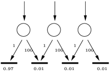
Figure 2: System with three customer types whose underload equilibrium is unstable.

On the other hand, we compute by Lemma 3.3

$$A_{u}=\pmatrix{-1.99&-0.99&-0.99\cr 97.02&-2.98&-1.98\cr 96.03&96.03&-3.97}$$

with eigenvalues $\{-17.8,4.45\pm 23.4i\}$. Therefore by Theorem 3.1, the system with these parameters is described by an unstable ODE in the neighborhood of its equilibrium point.

We now show that this is a minimal instability example, in the sense made precise by the following:

Lemma 5.2

Consider an underloaded system, $\rho<1$.

Let $I\geq 2$. Any customer type $i$ that is a leaf in the basic activity tree, does not affect the local stability of the system. Namely, let us modify the system by removing type $i$, and then modifying (if necessary) input rates $\lambda_{k}$ of the remaining types $k\in{\mathcal{I}}\setminus i$ so that the basic activity tree of the modified system is ${\mathcal{E}}\setminus(ij)$, where $(ij)$ is the (only) edge in ${\mathcal{E}}$ adjacent to $i$. Then, the original system is locally stable if and only if the modified one is.

A system with two (or one) nonleaf customer types is locally stable.

(i) If type $i$ is a leaf, the equation for $\psi_{i}(t)$ is simply $\dot{\psi}_{i}(t)=\lambda_{i}-\mu_{ij}\psi_{i}(t)$. This means (setting $i=1$) that $(1,0,\ldots,0)^{\dagger}$ is an eigenvector of $A_{u}$ with eigenvalue $-\mu_{ij}$. Further, it is easy to see that: (a) the rest of the eigenvalues of $A_{u}$ are those of matrix $A_{u}^{(-i)}$ obtained from $A_{u}$ by removing the first row and first column; and (b) $A_{u}^{(-i)}$ is exactly the “$A_{u}$-matrix” for the modified system.

(ii) We can assume that there are no customer-type leaves. The case $I=1$ is trivial (and is covered by Theorem 4.1), so let $I=2$. Throughout the proof, the pool sizes $\beta_{j}$ are fixed. From Theorem 4.1 we know that for a certain set of service rate values [namely, $\mu_{ij}=\mu_{j}$, $(ij)\in{\mathcal{E}}$], the matrix $A_{u}$ is stable. Suppose that we continuously vary the parameters $\mu_{ij}$ from those initial values to the values of interest, without ever making $\mu_{ij}=0$. If we assume that the final matrix $A_{u}$ is not stable, then as we change $\mu_{ij}$ the (changing) matrix $A_{u}$ acquires at some point two purely imaginary eigenvalues. If the eigenvalues of $A_{u}$ are purely imaginary, we must have $\operatorname{trace}(A_{u})=0$. However, as seen from the form of $A_{u}$ in Lemma 3.3, the diagonal entries of $A_{u}$ are always negative, and therefore $\operatorname{trace}(A_{u})<0$. The contradiction completes the proof.

An argument similar to the above proof also allows us to explain how the instability example 1 was found. In degree 3, let the characteristic polynomial of $A_{u}$ be $x^{3}-c_{2}x^{2}+c_{1}x-c_{0}$. A necessary and sufficient condition for all roots of the polynomial to have negative real parts is: $-c_{2},c_{1},-c_{0}>0$ and $c_{2}c_{1}<c_{0}$; see Farkas , Theorem 6. A necessary and sufficient condition for the “boundary case” between stability and instability (i.e., the condition for a pair of conjugate purely imaginary roots) is $c_{2}c_{1}=c_{0}$. Using Lemma 3.3 we can evaluate the characteristic polynomial symbolically and use the resulting expression to find parameters for which $c_{2}c_{1}=c_{0}$ will hold. See onlinecomputations online for the computations.

It is possible to construct an instability example with more reasonable values of $\beta_{j}$, $\mu_{ij}$, although it will be bigger. Figure 3 shows the diagram. The associated matrix $A_{u}$ and its eigenvalues can also be found online onlinecomputations .

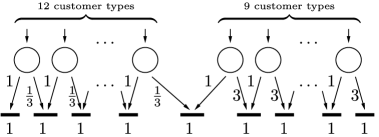
Figure 3: System with $\beta_{j}=1$ and $\mu_{ij}\in\{1/3,1,3\}$ whose underload equilibrium is unstable. There are 21 customer types.

We do not have an explicit characterization of the local instability domain, beyond the necessity of $I\geq 3$.

We now analyze the critically loaded system $\rho=1$ with queues, that is, the stability of the matrix $A_{c}$. Recall that the transformation $A_{c}$, restricted to subspace $\{y|\sum_{i}y_{i}=0\}$, and then the stability of $A_{c}$, does not depend on the values of $\beta_{j}$, so it suffices to specify the values $\mu_{ij}$.

Local instability example 2. Consider the network of Figure 4, which has 5 customer types $A$ through $E$ and 4 server types $1$ through $4$, connected $A-1-B-2-C-3-D-4-E$, with the following parameters:

$$\mu_{A1} = 1,\qquad\mu_{B1}=100,\qquad\mu_{B2}=1,\qquad\mu_{C2}=100,$$

$$\mu_{C3} = 1,\qquad\mu_{D3}=100,\qquad\mu_{D4}=10\mbox{,}000,\qquad\mu_{E4}=100.$$

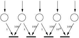
Figure 4: System with five customer types whose critical load equilibrium is unstable.

The matrix $A_{c}$, computed from Lemma 3.4 will be given by

$$A_{c}=\frac{1}{20}\pmatrix{9389&9805&10\mbox{,}201&10\mbox{,}597&-29\mbox{,}003\cr 10\mbox{,}894&9290&9706&10\mbox{,}102&-29\mbox{,}498\cr 10\mbox{,}399&10\mbox{,}795&9191&9607&-29\mbox{,}993\cr-40\mbox{,}091&-39\mbox{,}695&-39\mbox{,}299&-40\mbox{,}903&119\mbox{,}497\cr 9409&9805&10\mbox{,}201&10\mbox{,}597&-31\mbox{,}003}$$

and the eigenvalues of $A_{c}$ are $\{0,-16.88,-2190.05,2.565\pm 23.23i\}$.

Again, the above example 2 is in a sense minimal:

Lemma 5.3

Consider a critically loaded system, $\rho=1$.

Let $J\geq 2$. Any server type $j$ that is a leaf in the basic activity tree does not affect the local stability of the system. Namely, let us modify the system by removing type $j$, and then replacing $\lambda_{i}$ for the unique $i$ adjacent to $j$ by $\lambda_{i}-\beta_{j}\mu_{ij}$. Then, the original system is locally stable if and only if the modified one is.

Consider a system labeled $S$. We say that a system $S^{\prime}$ is an expansion of system $S$ if it is obtained from $S$ by the following modification. We pick one server type $j$ and one customer type $i$ adjacent to it in ${\mathcal{E}}$; we “split” type $j$ into two types $j^{\prime}$ and $j^{\prime\prime}$; we “connect” type $i$ to both $j^{\prime}$ and $j^{\prime\prime}$; each of the remaining types $i^{\prime}\in{\mathcal{C}}(j)\setminus i$ we connect to either $j^{\prime}$ or $j^{\prime\prime}$ (but not both); if $(i^{\prime}j^{\prime})$ [resp., $(i^{\prime}j^{\prime\prime})$] is a new edge, we set $\mu_{i^{\prime}j^{\prime}}=\mu_{i^{\prime}j}$ (resp., $\mu_{i^{\prime}j^{\prime\prime}}=\mu_{i^{\prime}j}$). Then, $S$ is locally stable if and only if $S^{\prime}$ is.

A system with four or fewer customer types is locally stable.

(i) The argument here is a “special case” of the one used to show the independence of transformation $A_{c}$ [restricted to $(I-1)$-dimensional invariant subspace] from $(\beta_{j})$ in the proof of Lemma 3.4. Namely, it is easy to check that the original system and the modified system share exactly same ODE (14).

i(ii) Again, it is easy to see that the two systems share the same ODE (14).

(iii) We can assume that there are no server-type leaves, so that the tree ${\mathcal{E}}$ has only customer-type leaves, of which it can have two, three, or four.

If it has four customer-type leaves, then the tree has a total of four edges, hence five nodes, that is, a single server pool, to which all the customer types are connected.

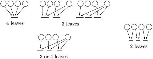
Figure 5: Possible arrangements of four customer types.

If the tree has three customer-type leaves, then letting $k$ be the number of edges from the fourth customer type, we have $k+3$ total edges, so $k+4$ nodes, of which $k$ are server types. That is, the nonleaf customer type is connected to all of the server types. Since there are no server-type leaves, we must have $k\leq 3$; since we are assuming the fourth customer type is not a leaf, we must have $k\geq 2$; thus, $k=2$ or $k=3$.

The last case is of two customer-type leaves. Letting $k,l$ be the number of edges coming out of the other customer types, we have $k+l+2$ edges. On the other hand, since each server type has at least 2 edges coming out of it, we have at most $(k+l+2)/2$ server types, so at most $(k+l+2)/2+4$ nodes. Thus, we have $(k+l+2)+1\leq(k+l+2)/2+4$, or $k+l+2\leq 6$, giving $k=l=2$ (since they must both be $\geq 2$).

We summarize the possibilities in Figure 5. Note that the bottom-left system can be obtained by a sequence of expansions from each of the top-left systems, and so this is the only system we need to consider to establish local stability for all 3- and 4-leaf cases. Thus, in total, the only two systems that need to be considered are bottom-left and right. In both of the resulting cases, we can use Lemma 3.4 to write out $A_{c}$ and its characteristic polynomial explicitly. The characteristic polynomial will have degree 4, but one of its roots is 0, so we can reduce it to degree 3. We then symbolically verify that the cited above stability criterion (Farkas , Theorem 6) for degree 3 polynomials, is satisfied. See onlinecomputations online for the details.

An argument similar to that in the above proof allows us to explain how the instability example 2 was found. We seek a condition satisfied by the coefficients of a degree 4 polynomial with two imaginary roots. Letting the polynomial be $x^{4}-c_{1}x^{3}+c_{2}x^{2}-c_{3}x+c_{4}$, and letting the roots be $\eta_{1}$, $\eta_{2}$, $\pm iz$ (where $\eta_{1}$ and $\eta_{2}$ may be real or complex conjugates, and $z\in{\mathbb{R}}$), we see that $c_{1}=\eta_{1}+\eta_{2}$, $c_{2}=\eta_{1}\eta_{2}+z^{2}$, $c_{3}=(\eta_{1}+\eta_{2})z^{2}$ and $c_{4}=\eta_{1}\eta_{2}z^{2}$. This implies the relation $c_{4}c_{1}^{2}+c_{3}^{2}-c_{1}c_{2}c_{3}=0$, and we can find the parameters for which this is true. (The symbolic calculation will involve rather a lot of terms.) We remark that, whereas for degree 3 polynomials the condition $c_{2}c_{1}-c_{0}=0$ is necessary and sufficient for the existence of two imaginary roots (Farkas , Theorem 6), the condition we derive here for degree 4 polynomials is necessary, but not sufficient. [E.g., the polynomial $(x-1)^{2}(x+1)^{2}$ has $c_{1}=c_{3}=0$, so $c_{4}c_{1}^{2}+c_{3}^{2}-c_{1}c_{2}c_{3}=0$, but it has no imaginary roots.] Thus, checking the sign of the corresponding expression alone is insufficient to determine whether the system is unstable, but is a useful way of narrowing down the parameter ranges.

Finally, it is possible to construct a single system which will be unstable both for $\rho<1$ and for $\rho=1$ with positive queues. For the local stability of the underloaded system, the leaves of the basic activity tree corresponding to customer types are irrelevant (the corresponding occupancy on the sole available server class converges to nominal exponentially). On the other hand, for the critically loaded system, the leaves corresponding to server pools are irrelevant, since the corresponding server is fully occupied by its unique available customer type. This observation allows us to merge the above two systems into a single one which is unstable both in underloaded and in the critically loaded case.

Consider a system with 5 customer types $A$ through $E$ and 5 server types $0$ through $4$ connected as $0-A-1-B-2-C-3-D-4-E$, with $\mu_{A0}=100$ and the remaining $\mu_{ij}$ as in the critically loaded case. Set $\beta_{3}=0.96$ while $\beta_{0},\beta_{1},\beta_{2},\beta_{4}=0.01$; see Figure 6.

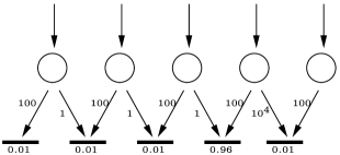
Figure 6: System with five customer types whose underload and critical load equilibrium points are both unstable.

By the above discussion, this system must be unstable for $\rho=1$ and positive queues. We therefore need to consider only the first 4 customer types ($E$ is a customer-type leaf and does not matter) in underload. We compute

$$A_{u}=\pmatrix{-1.99&-0.99&-0.99&-0.99\cr 97.02&-2.98&-1.98&-1.98\cr 96.03&96.03&-3.97&-2.97\cr-99&-99&-99&-199}$$

and eigenvalues are $\{-14.6,-201.1,3.91\pm 18.1i\}$.

While we showed above that sufficiently small systems are at least locally stable, we will show now that, in the underload case, any sufficiently large system is locally unstable for some parameter settings.

Lemma 5.4

In underload ($\rho<1$), any shape of basic activity tree that includes a locally unstable system (i.e., with $A_{u}$ having an eigenvalue with positive real part) as a subset will, with some set of parameters $(\beta_{j})$, $(\mu_{ij})$, become locally unstable. In particular, any shape of basic activity tree that includes instability example 1 (Figure 2) above (for $\rho<1$) will be locally unstable for some set of parameters $\beta_{j}$, $\mu_{ij}$.

Let $U$ be any system whose underload ($\rho<1$) equilibrium is locally unstable, for example, one of the examples given above, with the associated fixed set of parameters $\mu_{ij}$, $\beta_{j}$ and $\lambda_{i}$. Let $S$ be a system including $U$ as a subset, namely: the activity tree of $S$ is a superset of that of $U$; the $\mu_{ij}$ and $\beta_{j}$ in $U$ are preserved in $S$; the $\mu_{ij}$ in $S$ are fixed. Consider a sequence of systems $S^{\varepsilon}$ in which $\beta_{j}=\varepsilon\to 0$ for all $j$ not in $U$. For each $\varepsilon$, take $\lambda_{i}^{\varepsilon}$ so that all of the activities are indeed basic, and such that, as $\varepsilon\to 0$, $\lambda_{i}^{\varepsilon}\to\lambda_{i}$ for $i$ in $U$, and $\lambda_{i}^{\varepsilon}\to 0$ for $i$ not in $U$; see Remark 5.1. Order the $\psi_{i}$ so that the customer types $i$ in $U$ come first. Suppose there are $I$ customer types in $U$, and $I+k$ customer types in $S$. Let $A_{u}^{\varepsilon}$ be the $(I+k)\times(I+k)$ matrix associated with $S^{\varepsilon}$, and let $A_{u}$ be the $I\times I$ matrix associated with $U$ considered as an isolated system. Then as $\varepsilon\to 0$ the top left $I\times I$ entries of $A_{u}^{\varepsilon}$ converge to $A_{u}$, while the bottom left $k\times I$ entries of $A_{u}^{\varepsilon}$ converge to 0 (i.e., the effect of $U$ on the stability of the rest of the system vanishes—this is due to the fact that pool size parameters $\beta_{j}$ in $U$ remain constant, while $\beta_{j}\to 0$ in the rest of the system). Consequently, each eigenvalue of $A_{u}$ is a limit of eigenvalues of $A_{u}^{\varepsilon}$. Since $A_{u}$ had an eigenvalue with positive real part, for sufficiently small $\varepsilon$ the matrix $A_{u}^{\varepsilon}$ will have at least one eigenvalue with positive real part as well, so the system $S^{\varepsilon}$ will be locally unstable.

6 Diffusion scaled process in an underloaded system. Possible evanescence of invariant distributions

Above we have shown that on a fluid scale, around the equilibrium point, the system converges to a subset of its possible states, on which it evolves according to a differential equation, possibly unstable. This strongly suggests that, when the differential equation is unstable, the stochastic system is in fact “never” close to equilibrium. Our goal in this section is to demonstrate that it is the case at least on the diffusion scale. More precisely, we consider the system in underload, $\rho<1$, and look at diffusion-scaled stationary distributions (centered at the equilibrium point and scaled down by $\sqrt{r}$); we show that, when the associated fluid model is locally unstable, this sequence of stationary distributions is such that the measure of any compact set vanishes.

6.1 Transient behavior of diffusion scaled process. State space collapse

In this section we cite the diffusion limit result (for the process transient behavior) that we will need from GurvichWhitt . Again, we consider a sequence of systems indexed by $r$, with the input rates being $\lambda^{r}_{i}=r\lambda_{i}$, server pool sizes being $\beta_{j}r$, and the service rates $\mu_{ij}$ unchanged with $r$. [Here we drop the $o(r)$ terms in $\lambda^{r}_{i}=r\lambda_{i}+o(r)$, because, when $\rho<1$, considering these terms does not make sense.] The notation for the unscaled processes is the same as in the previous section; however, we are now interested in a different—diffusion—scaling. We define

$$\hat{\Psi}^{r}_{ij}(t) = \frac{\Psi^{r}_{ij}(t)-r\psi_{ij}^{*}}{\sqrt{r}},\qquad\hat{\Psi}^{r}_{i}(t)=\sum_{j}\hat{\Psi}^{r}_{ij}(t),$$

$$\hat{\Psi}^{r}_{j}(t) = \sum_{i}\hat{\Psi}^{r}_{ij}(t)=\frac{\Psi^{r}_{j}(t)-\rho r\beta_{j}}{\sqrt{r}}.$$

We will denote by $M^{\prime}$ the linear mapping from $z=(z_{ij},(ij)\in{\mathcal{E}})\in{\mathbb{R}}^{I+J-1}$ to $y=(y_{i})\in{\mathbb{R}}^{I}$, given by $\sum_{j}z_{ij}=y_{i}$. [So, $(\hat{\Psi}^{r}_{i}(t))\equiv M^{\prime}(\hat{\Psi}^{r}_{ij}(t))$.] There is the obvious relation between $M^{\prime}$ and the operator $M$ defined by (7): $M^{\prime}My=y$ for any $y\in{\mathbb{R}}^{I}$. Let us define ${\mathcal{M}}:=\{My|y\in{\mathbb{R}}^{I}\}$, an $I$-dimensional linear subspace of ${\mathbb{R}}^{I+J-1}$; equivalently, ${\mathcal{M}}=\{z\in{\mathbb{R}}^{I+J-1}|z=MM^{\prime}z\}$.

Theorem 6.1 ((Essentially a corollary of Theorems 3.1 and 4.4 in GurvichWhitt ))

Let $\rho<1$. Assume that as $r\to\infty$, $\hat{\Psi}^{r}_{\mathcal{E}}(0)\to\hat{\Psi}_{\mathcal{E}}(0)$ where $\hat{\Psi}_{\mathcal{E}}(0)$ is deterministic and finite. [Consequently, $\hat{\Psi}^{r}_{\mathcal{I}}(0)\to\hat{\Psi}_{\mathcal{I}}(0)=M^{\prime}\hat{\Psi}_{\mathcal{E}}(0)$.] Then,

$$\hat{\Psi}^{r}_{\mathcal{I}}(\cdot)\Longrightarrow\hat{\Psi}_{\mathcal{I}}(\cdot)\qquad\mbox{in $D^{I}[0,\infty)$}$$ (19)

and for any fixed $\eta>0$,

$$\hat{\Psi}^{r}_{\mathcal{E}}(\cdot)\Longrightarrow M\hat{\Psi}_{\mathcal{I}}(\cdot)\qquad\mbox{in $D^{I+J-1}[\eta,\infty)$},$$ (20)

where $\hat{\Psi}_{\mathcal{I}}(\cdot)$ is the unique solution of the SDE

$$\qquad\hat{\Psi}_{i}(t)=\hat{\Psi}_{i}(0)-\sum_{j\in{\mathcal{S}}(i)}\mu_{ij}\int_{0}^{t}\bigl{(}M\hat{\Psi}_{\mathcal{I}}(s)\bigr{)}_{ij}\,ds+\sqrt{2\lambda_{i}}B_{i}(t),\qquad i\in{\mathcal{I}},$$ (21)

and the processes $B_{i}(\cdot)$ are independent standard Brownian motions.

Recalling the definition of matrix $A_{u}$ [see (9)], (21) can be written as

$$\hat{\Psi}_{\mathcal{I}}(t)=\hat{\Psi}_{\mathcal{I}}(0)+\int_{0}^{t}A_{u}\hat{\Psi}_{\mathcal{I}}(s)\,ds+\bigl{(}\sqrt{2\lambda_{i}}B_{i}(t)\bigr{)}.$$ (22)

The meaning of Theorem 6.1 is simple: the diffusion limit of the process $\hat{\Psi}^{r}_{\mathcal{I}}(\cdot)$ is such that, at initial time $0$, it “instantly jumps” to the state $MM^{\prime}\hat{\Psi}_{\mathcal{E}}(0)$ on the manifold ${\mathcal{M}}$ [where $MM^{\prime}\hat{\Psi}_{\mathcal{E}}(0)=\hat{\Psi}_{\mathcal{E}}(0)$ only if $\hat{\Psi}_{\mathcal{E}}(0)\in{\mathcal{M}}$]; after this initial jump, the process stays on ${\mathcal{M}}$ and evolves according to SDE (22). Theorem 6.1 is “essentially a corollary” of results in GurvichWhitt , because the setting in GurvichWhitt is such that $\rho=1$, while we assumed $\rho<1$. However, our Theorem 6.1 can be proved the same way, and in a sense is easier, because when $\rho<1$, the queues vanish in the limit (which is why the queue length process is not even present in the statement of Theorem 6.1).

6.2 Evanescence of invariant measures

In this section we show that if the matrix $A_{u}$ has eigenvalues with positive real part, the stationary distribution of the (diffusion scaled) process $\hat{\Psi}^{r}_{\mathcal{E}}(\cdot)$ escapes to infinity as $r\to\infty$. Namely, we prove the following:

Theorem 6.2

Suppose $\rho<1$. Consider a sequence of systems as defined in Section 6.1, and denote by $\mu^{r}$ the stationary distribution of the process $\hat{\Psi}^{r}_{\mathcal{E}}(\cdot)$, a probability measure on ${\mathbb{R}}^{I+J-1}$. Let $b_{K}=\{|z|\leq K\}\subset{\mathbb{R}}^{I+J-1}$. Suppose the matrix $A_{u}$ has eigenvalues with positive real parts and no pure imaginary eigenvalues. Then for any $K$, $\mu^{r}(b_{K})\to 0$ as $r\to\infty$.

Before we proceed with the proof, let us introduce more notation and one auxiliary result. Let ${\mathcal{C}}_{\mathcal{I}}$ be the submanifold of convergence (stability) of ODE $(d/dt)y=A_{u}y$ on ${\mathbb{R}}^{I}$; namely, ${\mathcal{C}}_{\mathcal{I}}$ is the (real) subspace of ${\mathbb{R}}^{I}$ spanned by the Jordan basis vectors for matrix $A_{u}$ corresponding to all eigenvalues with negative real parts. Given assumptions of the theorem on $A_{u}$, the solutions to $(d/dt)y=A_{u}y$ converge to $0$ exponentially fast if $y(0)\in{\mathcal{C}}_{\mathcal{I}}$, and go to infinity exponentially fast if $y(0)\in{\mathbb{R}}^{I}\setminus{\mathcal{C}}_{\mathcal{I}}$. Let ${\mathcal{C}}=M{\mathcal{C}}_{\mathcal{I}}$ denote the corresponding submanifold of convergence (stability) of the linear ODE $(d/dt)z=(MA_{u}M^{\prime})z$ on $z\in{\mathcal{M}}$. This ODE is just the $M$-image of ODE $(d/dt)y=A_{u}y$. Therefore, a solution $z(t)$ converges to $0$ exponentially fast if $z(0)\in{\mathcal{C}}$, and goes to infinity exponentially fast if $z(0)\in{\mathcal{M}}\setminus{\mathcal{C}}$. Let us denote $b_{K}(\delta_{1},\delta_{2}):=b_{K}\cap\{d(z,{\mathcal{M}})\leq\delta_{1},d(z,{\mathcal{C}})\geq\delta_{2}\}$, where $d(\cdot,\cdot)$ is Euclidean distance.

Lemma 6.3

Solutions to SDE (22) have the following properties:

For any $T>0$ and any $\Psi_{\mathcal{I}}(0)$,

$${\mathbb{P}}\bigl{\{}M\hat{\Psi}_{\mathcal{I}}(T)\in{\mathcal{M}}\setminus{\mathcal{C}}\bigr{\}}=1;$$

For any $K>0$, $\delta_{2}>0$ and $\varepsilon>0$, there exist sufficiently large $T_{K}$ and $K^{\prime}>K$, such that, uniformly on $M\hat{\Psi}_{\mathcal{I}}(0)\in b_{K}(0,\delta_{2})$,

$${\mathbb{P}}\bigl{\{}M\hat{\Psi}_{\mathcal{I}}(T_{K})\in b_{K^{\prime}}\setminus b_{2K}\bigr{\}}\geq 1-\varepsilon.$$

Statement (i) follows from the fact that, regardless of the (deterministic) initial state $\Psi_{\mathcal{I}}(0)$, the solution to SDE (22) is such that the distribution of $\Psi_{\mathcal{I}}(T)$ is Gaussian with nonsingular covariance matrix. (See KaratzasShreve , Section 5.6. In our case the matrix of diffusion coefficients is diagonal with entries $\sqrt{2\lambda_{i}}$.) Therefore, the probability that $\Psi_{\mathcal{I}}(T)$ is in a subspace of lower dimension is zero.

Statement (ii) follows from the fact (again, see KaratzasShreve , Section 5.6) that the expectation $m(t)={\mathbb{E}}\hat{\Psi}_{\mathcal{I}}(t)$ evolves according to ODE

$$\dot{m}(t)=A_{u}m(t).$$

Since $d(M\hat{\Psi}_{\mathcal{I}}(0),{\mathcal{C}})\geq\delta_{2}$ [and thus $\hat{\Psi}_{\mathcal{I}}(0)$ is also separated by a positive distance from ${\mathcal{C}}_{\mathcal{I}}$], we have

$$\bigl{|}m(t)\bigr{|}\geq a_{1}\exp(at)$$

for some fixed $a_{1},a>0$ and all large $t$. [Here $a_{1}$ depends on the minimum length of the projection of $\hat{\Psi}_{\mathcal{I}}(0)$ along ${\mathcal{C}}_{\mathcal{I}}$ onto the (real) span of the Jordan basis vectors of $A_{u}$ corresponding to eigenvalues with positive real part, and $a$ is the smallest positive real part of an eigenvalue of $A_{u}$.] It is easy to check that if the mean of a Gaussian distribution goes to infinity, then (regardless of how the covariance matrix changes) the measure of any bounded set goes to zero. On the other hand, both $m(t)$ and the covariance matrix remain bounded for all $t\in[0,T_{K}]$, with any $T_{K}$; then, for any $T_{K}$, we can always choose $K^{\prime}$ large enough so that ${\mathbb{P}}\{M\hat{\Psi}_{\mathcal{I}}(T_{K})\in b_{K^{\prime}}\}$ is arbitrarily close to $1$. Proof of Theorem 6.2 We will consider measures $\mu^{r}$ as measures on the one-point compactification $\overline{\mathbb{R}}{}^{n}=\mathbb{R}^{n}\cup\{*\}$ of the space $\mathbb{R}^{n}$, where $n=I+J-1$. In this space, any subsequence of $\{\mu^{r}\}$ has a further subsequence, along which $\mu^{r}\stackrel{{\scriptstyle w}}{{\rightarrow}}\mu$ for some probability measure $\mu$ on $\overline{\mathbb{R}}{}^{n}$. We will show that the entire measure $\mu$ is concentrated on the infinity point $*$, that is, $\mu(\mathbb{R}^{n})=0$. Suppose not, that is, $\mu(\mathbb{R}^{n})>0$. The proof proceeds in two steps.

Step 1. We prove that $\mu(\mathbb{R}^{n})=\mu({\mathcal{M}}\setminus{\mathcal{C}})$. Indeed, let us choose any $\varepsilon>0$, and $K$ large enough so that $\mu(b_{K/2})>(1-\varepsilon)\mu(\mathbb{R}^{n})$. Then, for all large $r$, $\mu^{r}(b_{K})>(1-\varepsilon)\mu(\mathbb{R}^{n})$. Choose $\delta_{1}>0$ and $T>0$ arbitrary. From the properties of the limiting diffusion process (Lemma 6.3), we see that we can choose a sufficiently small $\delta_{2}>0$ and sufficiently large $K^{\prime}$ such that, uniformly on the initial states $\hat{\Psi}^{r}_{\mathcal{E}}(0)\in b_{K}$,

$$\liminf_{r\to\infty}{\mathbb{P}}\bigl{\{}\hat{\Psi}^{r}_{\mathcal{E}}(T)\in b_{K^{\prime}}(\delta_{1},\delta_{2})\bigr{\}}>1-\varepsilon.$$

This implies that for all large $r$,

$$\mu^{r}\bigl{(}b_{K^{\prime}}(\delta_{1},\delta_{2})\bigr{)}>(1-\varepsilon)^{2}\mu\bigl{(}\mathbb{R}^{n}\bigr{)},$$

and then $\mu(b_{K^{\prime}}(\delta_{1},\delta_{2}))\geq(1-\varepsilon)^{2}\mu(\mathbb{R}^{n})$. Since $\varepsilon$ and $\delta_{1}$ were arbitrary, we conclude that $\mu(\mathbb{R}^{n})\leq\mu({\mathcal{M}}\setminus{\mathcal{C}})$, and then, obviously, the equality must hold.

Step 2. We show that, for any $K>0$, $\mu(\mathbb{R}^{n}\setminus b_{K})=\mu(\mathbb{R}^{n})$. [This is, of course, impossible when $\mu(\mathbb{R}^{n})>0$, and thus we obtain a contradiction.] It suffices to show that for any $\varepsilon>0$, we can choose a sufficiently large $K$, such that $\mu(\mathbb{R}^{n}\setminus b_{K})\geq(1-\varepsilon)^{2}\mu(\mathbb{R}^{n})$. Let us choose (using step 1) a large $K$ and a small $\delta_{2}>0$, such that $\mu(b_{K/2}(\delta_{1}/2,2\delta_{2}))>(1-\varepsilon)\mu(\mathbb{R}^{n})$ for any $\delta_{1}>0$. Then, for any fixed $\delta_{1}>0$, for all large $r$, $\mu^{r}(b_{K}(\delta_{1},\delta_{2}))>(1-\varepsilon)\mu(\mathbb{R}^{n})$. Now, using Lemma 6.3(ii), we can choose $K^{\prime}$ and $T_{K}$ sufficiently large, and then $\delta_{1}$ sufficiently small, so that, uniformly on the initial states $\hat{\Psi}^{r}_{\mathcal{E}}(0)\in b_{K}(\delta_{1},\delta_{2})$,

$$\liminf_{r\to\infty}{\mathbb{P}}\bigl{\{}\hat{\Psi}^{r}_{\mathcal{E}}(T_{K})\in b_{K^{\prime}}\setminus b_{2K}\bigr{\}}\geq 1-\varepsilon.$$

Therefore,

$$\mu^{r}(b_{K^{\prime}}\setminus b_{2K})>(1-\varepsilon)^{2}\mu\bigl{(}\mathbb{R}^{n}\bigr{)}$$

for all large $r$, and then for the limiting measure $\mu$ we must have $\mu(\mathbb{R}^{n}\setminus b_{K})\geq(1-\varepsilon)^{2}\mu(\mathbb{R}^{n})$.

7 Diffusion scaled process in a critically loaded system in Halfin–Whitt asymptotic regime

In this section we consider the following asymptotic regime. The system is critically loaded, that is, the optimal solution to SPP (1) is such that $\rho=1$. As scaling parameter $r\to\infty$, assume that the server pool sizes are $r\beta_{j}$ (same as throughout the paper), and the input rates are $\lambda^{r}_{i}=r\lambda_{i}+\sqrt{r}l_{i}$, where the parameters (finite real numbers) $\{l_{i}\}$ are such that $\sum l_{i}\nu_{i}=-C<0$. Denote by $\rho^{r},\{\lambda^{r}_{ij}\}$ the optimal solution of SPP (1), with $\beta_{j}$’s and $\lambda_{i}$’s replaced by $r\beta_{j}$ and $\lambda_{i}^{r}$, respectively. (This solution is unique, as can be easily seen from the CRP condition.) Then, it is easy to check that $\rho^{r}=1+(\sum l_{i}\nu_{i})/\sqrt{r}=1-C/\sqrt{r}$, which in turn easily implies that, for any $r$, the system process is stable with the unique stationary distribution.

We use the definitions of (6.1) for the diffusion scaled variables, and add to them the following ones: $\hat{X}_{i}^{r}(t)=(X_{i}^{r}(t)-\psi_{i}^{*}r)/\sqrt{r}$ for the (diffusion-scaled) number of type $i$ customers; $\hat{Q}^{r}_{i}(t)=Q^{r}_{i}(t)/\sqrt{r}$ for the type $i$ queue length; $\hat{Z}^{r}_{j}(t)=Z^{r}_{j}(t)/\sqrt{r}$, where $Z^{r}_{j}(t)=\Psi^{r}_{j}(t)-r\beta_{j}\leq 0$ is the number of idle servers of type $j$ (with the minus sign). Note that, although the optimal average occupancy of pool $j$ is at $\rho^{r}r\beta_{j}$, the quantity $\hat{Z}^{r}_{j}(t)$ measures the deviation from full occupancy $r\beta_{j}$. Our choice of signs is such that $\hat{Q}^{r}_{i}\geq 0$ while $\hat{Z}^{r}_{j}\leq 0$. We will use the vector notations, such as $\hat{X}_{{\mathcal{I}}}^{r}(t)$, as usual.

Two main results of this section are as follows: (a) it is possible for the invariant distributions to escape to infinity under certain system parameters and (b) in the special case when service rate depends on the server type only, the invariant distributions are tight.

7.1 Example of evanescence of invariant measures

Recall that $\pi$ denotes the (matrix of) orthogonal projection on the subspace $L=\{y\in{\mathbb{R}}^{I}|\break\sum_{i}y_{i}=0\}$ in ${\mathbb{R}}^{I}$; this is the projection “along” the direction of vector $(1,\ldots,1)^{\dagger}$. Also recall the relation between matrices $A_{u}$ and $A_{c}$,

$$A_{c}=\pi A_{u}.$$

One more notation: for $y\in{\mathbb{R}}^{I}$,

$$F[y]=\cases{\pi y,&\quad if $\displaystyle\sum_{i}y_{i}>0$,\vspace*{2pt}\cr y,&\quad if $\displaystyle\sum_{i}y_{i}\leq 0$.}$$

Analogously to Theorem 6.1, the following fact is a corollary (this time—direct) of Theorems 3.1 and 4.4 in GurvichWhitt .

Theorem 7.1

Assume that as $r\to\infty$, $\hat{X}^{r}_{\mathcal{I}}(0)\to\hat{X}_{\mathcal{I}}(0)$ and $\hat{\Psi}^{r}_{\mathcal{E}}(0)\to\hat{\Psi}_{\mathcal{E}}(0)$, where $\hat{X}_{\mathcal{I}}(0)$ and $\hat{\Psi}_{\mathcal{E}}(0)$ are deterministic and finite. Then,

$$\hat{X}^{r}_{\mathcal{I}}(\cdot)\Longrightarrow\hat{X}_{\mathcal{I}}(\cdot)\qquad\mbox{in $D^{I}[0,\infty)$}$$ (23)

and for any fixed $\eta>0$,

$$\hat{\Psi}^{r}_{\mathcal{E}}(\cdot)\Longrightarrow MF\bigl{[}\hat{X}_{\mathcal{I}}(\cdot)\bigr{]}\qquad\mbox{in $D^{I+J-1}[\eta,\infty)$},$$ (24)

where $\hat{X}_{\mathcal{I}}(\cdot)$ is the unique solution of the SDE

$$\hat{X}_{\mathcal{I}}(t)=\hat{X}_{\mathcal{I}}(0)+\int_{0}^{t}A_{u}F\bigl{[}\hat{X}_{\mathcal{I}}(s)\bigr{]}\,ds+\bigl{(}\sqrt{2\lambda_{i}}B_{i}(t)\bigr{)},$$ (25)

and the processes $B_{i}(\cdot)$ are independent standard Brownian motions.

Next we establish the following fact.

Lemma 7.2

There exists a system and a parameter setting such that the following hold.

Matrix $A_{c}$ is unstable;

Matrix $A_{u}$ has $(1,\ldots,1)^{\dagger}$ as a right eigenvector, with real nonzero eigenvalue $c$,

$$A_{u}(1,\ldots,1)^{\dagger}=c(1,\ldots,1)^{\dagger}.$$ (26)

Let us start with the system in the local instability example 2 (see Figure 4) for the critical load. We will modify it as follows. We will change $\mu_{D3}$ from $100$ to $100-\varepsilon$ with sufficiently small positive $\varepsilon$, so that $A_{c}$ remains unstable. (The reason for this change will be explained shortly.) We will add two new server pools, 0 and 5, on the left and on the right, respectively, and set $\mu_{A0}=100$, $\mu_{E5}=1$; such addition of server-leaves does not change the instability of $A_{c}$. So, (i) holds.

Now, suppose all $\lambda_{i}$ are equal, say $\lambda_{i}=1$. We can choose $\psi_{ij}^{*}$ such that all $\psi_{i}^{*}=\sum_{j}\psi_{ij}^{*}$ are equal, and $\sum_{j}\mu_{ij}\psi_{ij}^{*}=\lambda_{i}=1$ for all $i$. Namely, we do the following. The reason for changing $\mu_{D3}$ from $100$ to $100-\varepsilon$ is to make it possible to choose $\psi_{D3}^{*}>0$ and $\psi_{D4}^{*}>0$, such that $\sum_{j}\mu_{Dj}\psi_{Dj}^{*}=1$ and $\psi_{D}^{*}=\psi_{D3}^{*}+\psi_{D4}^{*}>1/100$. We choose $\psi_{A0}^{*}=1/100-\delta$, $\psi_{A1}^{*}=100\delta$ (which guarantees $\sum_{j}\mu_{Aj}\psi_{Aj}^{*}=1$) with $\delta>0$ small enough so that $\psi_{A}^{*}=1/100+99\delta<1/(100-\varepsilon)$. The values of pairs $(\psi_{B1}^{*},\psi_{B2}^{*})$, $(\psi_{C2}^{*},\psi_{C3}^{*})$, $(\psi_{E4}^{*},\psi_{E5}^{*})$, are chosen to be equal to $(\psi_{A0}^{*},\psi_{A1}^{*})$. Finally, we choose $\psi_{D3}^{*}=(1-\delta_{1})/(100-\varepsilon)$ and $\psi_{D4}^{*}=\delta_{1}/10^{4}$ (which ensures $\sum_{j}\mu_{Dj}\psi_{Dj}^{*}=1$) with $\delta_{1}>0$ satisfying

$$\psi_{D}^{*}=(1-\delta_{1})/(100-\varepsilon)+\delta_{1}/10^{4}=1/100+99\delta=\psi_{A}^{*}.$$

This completes the choice of $\psi_{ij}^{*}$.

We set $\beta_{j}=\sum_{i}\psi_{ij}^{*}$. We see that $(\psi_{ij}^{*})$ is the equilibrium point. It follows from the construction that (26) will hold for $A_{u}$. Indeed, if $\psi_{{\mathcal{I}}}-\psi_{{\mathcal{I}}}^{*}=c_{1}(1,\ldots,1)^{\dagger}$, then $\psi_{{\mathcal{I}}}=c_{2}\psi_{{\mathcal{I}}}^{*}$, which in turn means that $\psi_{{\mathcal{E}}}=c_{2}\psi_{{\mathcal{E}}}^{*}$; therefore, the corresponding service rates are $\sum_{j}\mu_{ij}\psi_{ij}=c_{2}\sum_{j}\mu_{ij}\psi_{ij}^{*}=c_{2}\lambda_{i}=c_{2}$ for all $i$; therefore, $\dot{\psi}_{{\mathcal{I}}}=(1-c_{2})(1,\ldots,1)^{\dagger}$.

Theorem 7.3

Suppose we have a system with parameters satisfying Lemma 7.2, in the Halfin–Whitt regime, described in this section. Then, the sequence of stationary distributions of $\hat{X}_{\mathcal{I}}^{r}$ (and of $\hat{\Psi}_{\mathcal{I}}^{r}$) escapes to infinity: the measure of any compact set vanishes.

Since $(1,\ldots,1)^{\dagger}$ is an eigenvector of $A_{u}$, for any $y\in{\mathbb{R}}^{I}$ we have

$$\pi A_{u}F[y]=\pi A_{u}\pi y=A_{c}\pi y.$$

Then, taking the $\pi$-projection of equation (25), we see that $\pi\hat{X}_{\mathcal{I}}$ satisfies the following linear SDE

$$\pi\hat{X}_{\mathcal{I}}(t)=\pi\hat{X}_{\mathcal{I}}(0)+\int_{0}^{t}A_{c}\pi\hat{X}_{\mathcal{I}}(s)\,ds+\pi\bigl{(}\sqrt{2\lambda_{i}}B_{i}(t)\bigr{)}.$$ (27)

Given instability of linear equation (27), we can repeat the argument of Section 6.2 to show that the sequence of projections of the stationary distributions of $\hat{X}_{\mathcal{I}}^{r}$ on $L$ escapes to infinity.

7.2 Tightness of stationary distributions in the case when service rate depends on the server type only

In this section we consider a special case when there exists a set of positive rates $\{\mu_{j}\}$, such that $\mu_{ij}=\mu_{j}$ as long as $(ij)\in{\mathcal{E}}$. We demonstrate tightness of invariant distributions. (An analogous result holds for the underload system, $\rho<1$, as sketched out at the end of this section.) This, in combination with the transient diffusion limit results, allows us to claim that the limit of invariant distributions is the invariant distribution of the limiting diffusion process.

Theorem 7.4

Suppose $\mu_{ij}=\mu_{j},(ij)\in{\mathcal{E}}$ and $\rho=1$. Consider a system under the LQFS-LB rule in the asymptotic regime defined above in this section. Then, for any real

$$\theta<\theta_{0}:=\frac{2\min_{i}\lambda_{i}}{\sum_{i}\lambda_{i}+(\max_{j}\mu_{j})\sum_{j}\beta_{j}},$$

the stationary distributions are such that

$$\lim\sup_{r}{\mathbb{E}}\biggl{[}\sum_{i}\exp\bigl{(}\theta\hat{Q}^{r}_{i}\bigr{)}+\sum_{j}\beta_{j}\exp\bigl{(}\theta\hat{Z}^{r}_{j}/\beta_{j}\bigr{)}\biggr{]}<\infty.$$

Note that the statement is trivial for $\theta=0$. Also, for $\theta>0$ each term $\exp(\theta\hat{Z}^{r}_{j}/\beta_{j})$ is bounded so has finite expectation, while for $\theta<0$ each term $\exp(\theta\hat{Q}^{r}_{i})$ is bounded so has finite expectation.

Our method is related to that in GamarnikStolyar . (The exposition below is self-contained.)

Step 1: Preliminary bounds. Consider the embedded Markov chain taken at the instants of (say, right after) the transitions. We will use uniformization, that is, we keep the total rate of all transitions from any state constant at $\alpha^{r}r=\sum_{i}\lambda^{r}_{i}+\sum_{j}r\beta_{j}\mu^{*}$, where $\mu^{*}=\max\mu_{j}$; note that, as $r\to\infty$, $\alpha^{r}\to\alpha^{*}=\sum_{i}\lambda_{i}+\sum_{j}\beta_{j}\mu^{*}$. The transitions are of three types: arrivals, departures and virtual transitions, which do not change the state of the system. The rate of a transition due to a type $i$ arrival is $\lambda_{i}^{r}$; for the service completion at pool $j$ the rate is $\mu_{j}(r\beta_{j}+Z^{r}_{j})$ (recall $Z^{r}_{j}\leq 0$); and a virtual transition occurs at the complementary rate $\alpha^{r}r-\sum_{i}\lambda^{r}_{i}-\sum_{j}\mu_{j}(r\beta_{j}+Z^{r}_{j})$. (Obviously, the probability that a transition occurring at a transition instant has a given type is the ratio of the corresponding rate and $\alpha^{r}r$.) The stationary distribution of the embedded Markov chain is the same as that of the original, continuous-time chain.

In the rest of the proof, $\tau\in\{0,1,2,\ldots\}$ refers to the discrete time of the embedded Markov chain.

We will work with the following Lyapunov function:

$${\mathcal{L}}(\tau):=\sum_{i}\exp\bigl{(}\theta\hat{Q}^{r}_{i}(\tau)\bigr{)}+\sum_{j}\beta_{j}\exp\bigl{(}\theta\hat{Z}^{r}_{j}(\tau)/\beta_{j}\bigr{)}.$$ (28)

Throughout, we use the bound

$$\exp(\theta y)\leq\exp(\theta x)\bigl{(}1+\theta(y-x)+\tfrac 12\theta^{2}(y-x)^{2}\exp\bigl{(}\theta|y-x|\bigr{)}\bigr{)},$$ (29)

which arises from the second-order Taylor expansion of $\exp(\theta y)$.

A priori we do not know that ${\mathbb{E}}[{\mathcal{L}}(\tau)]$ exists for $\theta>0$. Indeed, while $\hat{Z}^{r}_{j}(t)$ is bounded for any $r$ (above by 0 and below by $-\beta_{j}\sqrt{r}$), the scaled queue size $\hat{Q}^{r}_{i}(t)$ is unbounded. To deal with this, we also consider the truncated Lyapunov function ${\mathcal{L}}^{K}=\min\{{\mathcal{L}},K\}$.

In the equation below, let $x$ denote the variable of interest (either $\hat{Q}^{r}_{i}$ or $\hat{Z}^{r}_{j}/\beta_{j}$), and let $S(\tau)$ denote the state of the embedded Markov chain at time $\tau$. From (29) we obtain

$${\mathbb{E}}\bigl{[}\exp\bigl{(}\theta x(\tau+1)\bigr{)}-\exp\bigl{(}\theta x(\tau)\bigr{)}|S(\tau)\bigr{]}$$

$$\qquad\leq\exp\bigl{(}\theta x(\tau)\bigr{)}\bigl{(}\theta{\mathbb{E}}\bigl{[}x(\tau+1)-x(\tau)|S(\tau)\bigr{]}$$

$$\hskip 52.5pt\qquad\quad{}+\tfrac 12\theta^{2}{\mathbb{E}}\bigl{[}\bigl{(}x(\tau+1)-x(\tau)\bigr{)}^{2}\exp\bigl{(}\theta\bigl{|}x(\tau+1)-x(\tau)\bigr{|}\bigr{)}|S(\tau)\bigr{]}\bigr{)}.$$

Since for both $\hat{Z}^{r}_{j}$ and $\hat{Q}^{r}_{i}$ the change in a single transition is bounded by $1/\sqrt{r}$, we conclude

$${\mathbb{E}}\bigl{[}\exp\bigl{(}\theta\hat{Q}_{i}^{r}(\tau+1)\bigr{)}-\exp\bigl{(}\theta\hat{Q}_{i}^{r}(\tau)\bigr{)}|S(\tau)\bigr{]}$$

$$\qquad\leq\exp\bigl{(}\theta\hat{Q}_{i}^{r}(\tau)\bigr{)}\biggl{(}\theta{\mathbb{E}}\bigl{[}\hat{Q}_{i}^{r}(\tau+1)-\hat{Q}_{i}^{r}(\tau)|S(\tau)\bigr{]}$$ (30)

$$\qquad\quad\hskip 94.1pt{}+\biggl{(}\frac{1}{2}\theta^{2}\exp(\theta/\sqrt{r})\biggr{)}\frac{1}{r}\biggr{)},$$

$${\mathbb{E}}\bigl{[}\beta_{j}\exp\bigl{(}\theta\hat{Z}_{j}^{r}(\tau+1)/\beta_{j}\bigr{)}-\beta_{j}\exp\bigl{(}\theta\hat{Z}_{j}^{r}(\tau)/\beta_{j}\bigr{)}|S(\tau)\bigr{]}$$

$$\qquad\leq\exp\bigl{(}\theta\hat{Z}_{j}^{r}(\tau)/\beta_{j}\bigr{)}\biggl{(}\theta{\mathbb{E}}\bigl{[}\hat{Z}_{j}^{r}(\tau+1)-\hat{Z}_{j}^{r}(\tau)|S(\tau)\bigr{]}$$ (31)

$$\qquad\quad\hskip 93.0pt{}+\biggl{(}\frac{1}{\beta_{j}}\frac{1}{2}\theta^{2}\exp(\theta/\sqrt{r})\biggr{)}\frac{1}{r}\biggr{)}.$$

Clearly, as long as values of $\theta$ are bounded, for any fixed $C_{2}>1$ and all sufficiently (depending on $C_{2}$) large $r$, the second summands in (7.2) and (7.2) are upper bounded by $C_{2}\frac{1}{2}\theta^{2}\frac{1}{r}$ and $\frac{1}{\beta_{*}}C_{2}\frac{1}{2}\theta^{2}\frac{1}{r}$, respectively, where $\beta_{*}=\min_{j}\beta_{j}$. Note that the second bound is independent of $j$.

Next, we will obtain an upper bound on the drift

$${\mathbb{E}}\bigl{[}{\mathcal{L}}(\tau+1)-{\mathcal{L}}(\tau)|S(\tau)\bigr{]}.$$

To do that, we introduce an artificial scheduling/routing rule, which acts only within one time step, and is such that the increment ${\mathcal{L}}(\tau+1)-{\mathcal{L}}(\tau)$ under this rule is “almost” a (pathwise, w.p.1) upper bound on this increment under the actual—LQFS-LB—rule. [It is important to keep in mind that the artificial rule is not a rule that is applied continuously. It is limited to one time step, and its sole purpose is to derive a pathwise upper bound on the increment ${\mathcal{L}}(\tau+1)-{\mathcal{L}}(\tau)$ within one time step.]

Step 2: Artificial scheduling/routing rule. We will use the following notation: ${\mathcal{I}}_{+}={\mathcal{I}}_{+}(\tau):=\{i\dvtx\hat{Q}^{r}_{i}(\tau)>0\}$, ${\mathcal{I}}_{0}={\mathcal{I}}_{0}(\tau):=\{i\dvtx\hat{Q}^{r}_{i}(\tau)=0\}$, ${\mathcal{J}}_{-}={\mathcal{J}}_{-}(\tau):=\{j\dvtx\hat{Z}^{r}_{j}(\tau)<0\}$, ${\mathcal{J}}_{0}={\mathcal{J}}_{0}(\tau):=\{j\dvtx\hat{Z}^{r}_{j}(\tau)=0\}$.

Scheduling: Departures from servers $j\in{\mathcal{J}}_{-}$ are processed normally, that is, reduce the corresponding $Z^{r}_{j}(\tau)$ by 1. Whenever there is a departure from a server pool $j\in{\mathcal{J}}_{0}$, the server takes up a customer of type $i$ with probability $\lambda^{r}_{ij}/\sum_{i}\lambda^{r}_{ij}$, keeping $Z^{r}_{j}(\tau+1)=0$ and reducing $Q^{r}_{i}(\tau+1)=Q^{r}_{i}(\tau)-1$. However, if it happens that the chosen $i$ is such that $Q^{r}_{i}(\tau)=0$, that is, $i\in{\mathcal{I}}_{0}$, then we keep $Q^{r}_{i}(\tau+1)=Q^{r}_{i}(\tau)=0$ and instead allow $Z^{r}_{j}(\tau+1)=-1$.

Routing: Arrivals to customer types $i\in{\mathcal{I}}_{+}$ are processed normally, that is, the corresponding $Q^{r}_{i}(\tau)$ is increased by 1. Whenever there is an arrival to a customer type $i\in{\mathcal{I}}_{0}$, it is routed to server pool $j$ with probability $\lambda^{r}_{ij}/\lambda^{r}_{i}$, keeping $Q^{r}_{i}(\tau+1)=Q^{r}_{i}(\tau)=0$ and increasing $Z^{r}_{j}(\tau+1)=Z^{r}_{j}(\tau)+1$. However, if it happens that the chosen $j$ is such that $Z^{r}_{j}(\tau)=0$, that is, $j\in{\mathcal{J}}_{0}$, then we keep $Z^{r}_{j}(\tau+1)=Z^{r}_{j}(\tau)=0$ and instead allow $Q^{r}_{i}(\tau+1)=1$.

Step 3: One time-step drift under the artificial rule. For $i\in{\mathcal{I}}_{+}$,

$${\mathbb{E}}\bigl{[}\hat{Q}^{r}_{i}(\tau+1)-\hat{Q}^{r}_{i}(\tau)|S(\tau)\bigr{]}=\frac{1}{\alpha^{r}r}\frac{1}{\sqrt{r}}\biggl{(}\lambda_{i}^{r}-\sum_{j}(\mu_{j}r\beta_{j})\frac{\lambda^{r}_{ij}}{\sum_{k}\lambda^{r}_{kj}}\biggr{)}$$

or, recalling that

$$\sum_{k}\lambda_{kj}^{r}=\mu_{j}\beta_{j}r\rho^{r}=\mu_{j}\beta_{j}r(1-C/\sqrt{r}),$$ (32)

we obtain

$${\mathbb{E}}\bigl{[}\hat{Q}^{r}_{i}(\tau+1)-\hat{Q}^{r}_{i}(\tau)|S(\tau)\bigr{]}=-\frac{C\lambda_{i}}{\alpha^{*}}\frac{1+o(1)}{r},\qquad i\in{\mathcal{I}}_{+},$$ (33)

where $o(1)$ is a fixed function, vanishing as $r\to\infty$.

If $\hat{Q}^{r}_{i}(\tau)=0$ (i.e., $i\in{\mathcal{I}}_{0}$), and a new type $i$ arrival is routed to pool $j$ with $\hat{Z}^{r}_{j}(\tau)<0$ (i.e., $j\in{\mathcal{J}}_{-}$), then of course $\hat{Q}^{r}_{i}$ stays at $0$ and $\hat{Q}^{r}_{i}(\tau+1)-\hat{Q}^{r}_{i}(\tau)=0$. However, if a new type $i$ arrival has to be routed to $j\in{\mathcal{J}}_{0}$, then (by the definition of artificial rule) $\hat{Q}^{r}_{i}(\tau+1)-\hat{Q}^{r}_{i}(\tau)=\hat{Q}^{r}_{i}(\tau+1)=1/\sqrt{r}$. Thus, we can write

$${\mathbb{E}}\bigl{[}\hat{Q}^{r}_{i}(\tau+1)-\hat{Q}^{r}_{i}(\tau)|S(\tau)\bigr{]}=\sum_{j\in{\mathcal{J}}_{0}}\frac{\lambda^{r}_{ij}}{\alpha^{r}r}\frac{1}{\sqrt{r}},\qquad i\in{\mathcal{I}}_{0}.$$ (34)

Note that the right-hand side of (34) is of order $1/\sqrt{r}$, not $1/r$. However, we will see shortly that order $1/\sqrt{r}$ terms in ${\mathbb{E}}[{\mathcal{L}}(\tau+1)-{\mathcal{L}}(\tau)|S(\tau)]$ cancel out, and this expected drift is in fact of order $1/r$.

The treatment of the drift of $\hat{Z}^{r}_{j}$ is similar [and again makes use of (32)]. We obtain

$$\qquad\quad{\mathbb{E}}\bigl{[}\hat{Z}^{r}_{j}(\tau+1)-\hat{Z}^{r}_{j}(\tau)|S(\tau)\bigr{]} = -\frac{1}{\alpha^{r}}\mu_{j}\bigl{(}\hat{Z}^{r}_{j}(\tau)+\beta_{j}C\bigr{)}\frac{1}{r},\qquad j\in{\mathcal{J}}_{-},$$ (35)

$${\mathbb{E}}\bigl{[}\hat{Z}^{r}_{j}(\tau+1)-\hat{Z}^{r}_{j}(\tau)|S(\tau)\bigr{]} = -\frac{1}{\sqrt{r}}\sum_{i\in{\mathcal{I}}_{0}}\frac{r\mu_{j}\beta_{j}}{\alpha^{r}r}\frac{\lambda^{r}_{ij}}{\sum_{k}\lambda^{r}_{kj}}$$

$$= -\frac{1}{1-C/\sqrt{r}}\sum_{i\in{\mathcal{I}}_{0}}\frac{\lambda^{r}_{ij}}{\alpha^{r}r}\frac{1}{\sqrt{r}},\qquad j\in{\mathcal{J}}_{0}.$$

We can rewrite (7.2) as

$${\mathbb{E}}\bigl{[}\hat{Z}^{r}_{j}(\tau+1)-\hat{Z}^{r}_{j}(\tau)|S(\tau)\bigr{]}$$

(37)

$$\qquad=-\sum_{i\in{\mathcal{I}}_{0}}\frac{\lambda^{r}_{ij}}{\alpha^{r}r}\frac{1}{\sqrt{r}}-\frac{C\sum_{i\in{\mathcal{I}}_{0}}\lambda_{ij}}{\alpha^{*}}\frac{1+o(1)}{r},\qquad j\in{\mathcal{J}}_{0},$$

where $o(1)$ is a fixed function, vanishing as $r\to\infty$.

Note that if ${\mathcal{L}}(\tau)\geq K$, then ${\mathcal{L}}^{K}(\tau+1)-{\mathcal{L}}^{K}(\tau)\leq 0$, and if ${\mathcal{L}}(\tau)<K$, then ${\mathcal{L}}^{K}(\tau+1)-{\mathcal{L}}^{K}(\tau)\leq{\mathcal{L}}(\tau+1)-{\mathcal{L}}(\tau)$. Putting together this observation and equations (7.2), (7.2), (33)–(7.2), we obtain

$${\mathbb{E}}\bigl{[}{\mathcal{L}}^{K}(\tau+1)-{\mathcal{L}}^{K}(\tau)|S(\tau)\bigr{]}$$ (38b)

$$\qquad\leq{\mathbf{1}}_{\{{\mathcal{L}}(\tau)\leq K\}}\biggl{(}\sum_{i\in{\mathcal{I}}_{+}}\exp\bigl{(}\theta\hat{Q}^{r}_{i}(\tau)\bigr{)}\theta\biggl{[}-\frac{C\lambda_{i}(1+o(1))}{\alpha^{*}}\biggr{]}\frac{1}{r}$$

$$\hskip 46.5pt\qquad\quad{}+\sum_{i\in{\mathcal{I}}_{0},j\in{\mathcal{J}}_{0}}\theta\lambda^{r}_{ij}\frac{1}{\alpha^{r}r}\frac{1}{\sqrt{r}}$$ (38g)

$$\hskip 46.5pt\qquad\quad{}+\sum_{j\in{\mathcal{J}}_{-}}\exp\bigl{(}\theta\hat{Z}^{r}_{j}(\tau)/\beta_{j}\bigr{)}\theta\biggl{[}-\frac{\mu_{j}}{\alpha^{r}}\biggr{]}\bigl{[}\hat{Z}^{r}_{j}(\tau)+\beta_{j}C\bigr{]}\frac{1}{r}$$

$$\hskip 46.5pt\qquad\quad{}+\sum_{j\in{\mathcal{J}}_{0},i\in{\mathcal{I}}_{0}}\theta\biggl{[}-\lambda^{r}_{ij}\frac{1}{\alpha^{r}r}\frac{1}{\sqrt{r}}-\frac{C\lambda_{i}(1+o(1))}{\alpha^{*}}\frac{1}{r}\biggr{]}$$

$$\hskip 46.5pt\qquad\quad{}+\sum_{i\in{\mathcal{I}}}\exp\bigl{(}\theta\hat{Q}^{r}_{i}(\tau)\bigr{)}\biggl{(}\frac{C_{2}}{2}\theta^{2}\biggr{)}\frac{1}{r}$$

$$\hskip 106.5pt\qquad\quad{}+\sum_{j\in{\mathcal{J}}}\frac{1}{\beta_{*}}\exp\bigl{(}\theta\hat{Z}^{r}_{j}(\tau)/\beta_{j}\bigr{)}\biggl{(}\frac{C_{2}}{2}\theta^{2}\biggr{)}\frac{1}{r}\biggr{)}.$$

Note that the $O(1/\sqrt{r})$ terms in (38g) and (38g) cancel each other as promised, so there are no $O(1/\sqrt{r})$ terms in the final bound.

Step 4: One time-step drift under the LQFS-LB rule. We now explain in what sense the increment ${\mathcal{L}}(\tau+1)-{\mathcal{L}}(\tau)$ under the artificial rule is “almost” an upper bound on this increment under LQFS-LB. To illustrate the idea, suppose first that all $\beta_{j}$ are equal. Then, it is easy to observe that for any fixed $S(\tau)$, the increment ${\mathcal{L}}(\tau+1)-{\mathcal{L}}(\tau)$ under the artificial rule is (with probability 1) an upper bound of this increment under LQFS-LB. Indeed, suppose first that a transition of the Markov chain is associated with a service completion in server pool $j$ with $\hat{Z}_{j}^{r}=0$. (If $\hat{Z}_{j}^{r}<0$, there is no difference in what the two rules do.) The only case of interest is when the LQFS-LB “takes” a new customer for service from queue $i$ with $\hat{Q}_{i}^{r}>0$, while the artificial rule tries to take a customer from a different queue $i^{\prime}$. Then $\hat{Q}_{i}^{r}\geq\hat{Q}_{i^{\prime}}^{r}$ must hold, with $\hat{Q}_{i}^{r}>\hat{Q}_{i^{\prime}}^{r}$ being the nontrivial case. If $\hat{Q}_{i^{\prime}}^{r}>0$, then the LQFS-LB will decrease the larger queue, and so the increment ${\mathcal{L}}(\tau+1)-{\mathcal{L}}(\tau)$ under the LQFS-LB is smaller (which is true for both positive and negative $\theta$). If $\hat{Q}_{i^{\prime}}^{r}=0$, then the LQFS-LB will still decrease queue $\hat{Q}_{i}^{r}$, while the artificial rule will instead decrease $\hat{Z}_{j}^{r}$; using convexity of $e^{\theta x}$, we verify that, again, the increment ${\mathcal{L}}(\tau+1)-{\mathcal{L}}(\tau)$ under the LQFS-LB is smaller (for both positive and negative $\theta$). If transition of the Markov chain is associated with a new customer arrival, we use an analogous argument to show that, again, the increment ${\mathcal{L}}(\tau+1)-{\mathcal{L}}(\tau)$ under the LQFS-LB cannot be greater than that under the artificial rule. We conclude that when all $\beta_{j}$ are equal, the key estimate (7.4) of the espected drift holds, in exactly same form, for LQFS-LB rule as well.

Now consider the case of general $\beta_{j}$. In the event of a service completion (and then possibly taking a customer for service from one of the nonzero queues), the increment ${\mathcal{L}}(\tau+1)-{\mathcal{L}}(\tau)$ under LQFS-LB is still no greater than under the artificial rule. (Verified similarly to the case of all $\beta_{j}$ being equal.) The only situation when LQFS-LB can possibly cause a greater increment than the artificial rule is as follows. There is an arrival of a type $i$ customer, which the artificial rule routes to pool $j$ with $\hat{Z}_{j}^{r}<0$, but the LQFS-LB will instead route it to pool $k$ such that $\hat{Z}_{j}^{r}/\beta_{j}\geq\hat{Z}_{k}^{r}/\beta_{k}$. Given convexity of function $e^{\theta x}$, the “worst case,” that is, the largest increment of ${\mathcal{L}}(\tau+1)-{\mathcal{L}}(\tau)$, occurs when $\hat{Z}_{k}^{r}$ is such that the equality holds, $\hat{Z}_{j}^{r}/\beta_{j}=\hat{Z}_{k}^{r}/\beta_{k}$. (If $\theta>0$ the positive increment gets larger, if we were to increase $\hat{Z}_{k}^{r}$; if $\theta<0$ the negative increment gets smaller in absolute value, if we were to increase $\hat{Z}_{k}^{r}$. Note also that here we allow $\hat{Z}_{k}^{r}$, determined by the equality, to be such that $Z_{k}^{r}=\hat{Z}_{k}^{r}\sqrt{r}$ is possibly noninteger, because we only use this value of $\hat{Z}_{k}^{r}$ to estimate the increment of a function.) Thus, as we replace the artificial rule by LQFS-LB, in the “worst case,” the increment

$$\beta_{j}\exp\bigl{(}\theta\bigl{[}\hat{Z}^{r}_{j}(\tau)+r^{-1/2}\bigr{]}/\beta_{j}\bigr{)}-\beta_{j}\exp\bigl{(}\theta\hat{Z}^{r}_{j}(\tau)/\beta_{j}\bigr{)}$$

may need to be replaced by

$$\beta_{k}\exp\bigl{(}\theta\bigl{[}\hat{Z}^{r}_{k}(\tau)+r^{-1/2}\bigr{]}/\beta_{k}\bigr{)}-\beta_{k}\exp\bigl{(}\theta\hat{Z}^{r}_{k}(\tau)/\beta_{k}\bigr{)}$$

with $\hat{Z}_{k}^{r}(\tau)$ satisfying $\hat{Z}_{j}^{r}(\tau)/\beta_{j}=\hat{Z}_{k}^{r}(\tau)/\beta_{k}$. In this case we obtain

$$\beta_{k}\exp\bigl{(}\theta\hat{Z}_{k}^{r}(\tau+1)/\beta_{k}\bigr{)}-\beta_{k}\exp\bigl{(}\theta\hat{Z}_{k}^{r}(\tau)/\beta_{k}\bigr{)}$$

$$\qquad\leq\exp\bigl{(}\theta\hat{Z}_{k}^{r}(\tau)/\beta_{k}\bigr{)}\biggl{(}\theta r^{-1/2}+\biggl{(}\frac{1}{\beta_{k}}\frac{1}{2}\theta^{2}\exp(\theta/\sqrt{r})\biggr{)}\frac{1}{r}\biggr{)}$$ (39)

$$\qquad\leq\exp\bigl{(}\theta\hat{Z}_{j}^{r}(\tau)/\beta_{j}\bigr{)}\biggl{(}\theta r^{-1/2}+\biggl{(}\frac{1}{\beta_{*}}\frac{1}{2}\theta^{2}\exp(\theta/\sqrt{r})\biggr{)}\frac{1}{r}\biggr{)},$$

This means that, under LQFS-LB rule, the estimate (7.4) still holds.

Step 5: Exponential moments estimates. Next, note that for each fixed $K>0$ and each fixed parameter $r$, the values of $\exp(\theta\hat{Q}^{r}_{i}(\tau))$ are uniformly bounded over all states $S(\tau)$ satisfying condition ${\mathcal{L}}(\tau)\leq K$; the values of $\exp(\theta\hat{Z}^{r}_{j}(\tau)/\beta_{j})$ are “automatically” uniformly bounded (for a fixed $r$). We take the expected values of both parts of (7.4) with respect to the invariant distribution. The expectation of the left-hand side is of course $0$, and so we get rid of the factor $1/r$ from the right-hand side expectation. The resulting estimates we will write separately for the cases $\theta>0$ and $\theta<0$ (with the case $\theta=0$ being trivial).

Case $\theta>0$. For a fixed $\theta>0$, the expected value of the sum of all terms not containing $\exp(\theta\hat{Q}^{r}_{i}(\tau))$ is bounded (uniformly in $r$). Indeed, this follows from the facts that $\hat{Z}^{r}_{j}(\tau)\leq 0$ and $0\leq-\theta\hat{Z}^{r}_{j}(\tau)\exp(\theta\hat{Z}^{r}_{j}(\tau)/\beta_{j})\leq\beta_{j}/e$ (because $0\geq xe^{x}\geq-\frac{1}{e}$ for $x\leq 0$). Then, we obtain

$${\mathbb{E}}\biggl{[}{\mathbf{1}}_{\{{\mathcal{L}}(\tau)\leq K\}}\sum_{i\in{\mathcal{I}}_{+}}\exp\bigl{(}\theta\hat{Q}^{r}_{i}(\tau)\bigr{)}\biggl{(}\frac{C\lambda_{i}(1+o(1))}{\alpha^{*}}\theta-\biggl{(}\frac{C_{2}}{2}\theta^{2}\biggr{)}\biggr{)}\biggr{]}\leq C_{1}$$ (40)

for some constant $C_{1}=C_{1}(\theta)>0$, uniformly on all sufficiently large $r$. Now let us fix a sufficiently small positive $\theta$, so that all coefficients of $\exp(\theta\hat{Q}^{r}_{i}(\tau))$ are at least some $\varepsilon>0$ (for all large $r$). Recalling that $C_{2}>1$ can be arbitrarily close to $1$, it suffices that $\theta<\theta_{0}=2(\min_{i}\lambda_{i})/\alpha^{*}$. Then,

$${\mathbb{E}}\biggl{[}{\mathbf{1}}_{\{{\mathcal{L}}(\tau)\leq K\}}\sum_{i\in{\mathcal{I}}_{+}}\exp\bigl{(}\theta\hat{Q}^{r}_{i}(\tau)\bigr{)}\biggr{]}\leq C_{1}/\varepsilon,$$

from where, letting $K\to\infty$, by monotone convergence, we obtain

$${\mathbb{E}}\biggl{[}\sum_{i\in{\mathcal{I}}_{+}}\exp\bigl{(}\theta\hat{Q}^{r}_{i}(\tau)\bigr{)}\biggr{]}\leq C_{1}/\varepsilon<\infty,$$ (41)

uniformly on all large $r$.

Case $\theta<0$. Fix arbitrary $\theta<0$. In this case, the expected value of the sum of all terms not containing $\exp(\theta\hat{Z}^{r}_{j}(\tau))$, is bounded (uniformly on $r$). We can write

$${\mathbb{E}}\biggl{[}{\mathbf{1}}_{\{{\mathcal{L}}(\tau)\leq K\}}\sum_{j\in{\mathcal{J}}_{-}}\exp\bigl{(}\theta\hat{Z}^{r}_{j}(\tau)/\beta_{j}\bigr{)}$$

(42)

$$\hskip 77.0pt{}\times\biggl{(}\theta\biggl{[}\frac{\mu_{j}}{\alpha^{r}}\biggr{]}\bigl{[}\hat{Z}^{r}_{j}(\tau)+\beta_{j}C\bigr{]}-\biggl{(}\frac{1}{\beta_{*}}\frac{C_{2}}{2}\theta^{2}\biggr{)}\biggr{)}\biggr{]}\leq C^{\prime}_{1}$$

for some constant $C^{\prime}_{1}=C^{\prime}_{1}(\theta)>0$, uniformly on all sufficiently large $r$. Let us choose sufficiently large $K_{1}>0$, such that the condition $\hat{Z}^{r}_{j}(\tau)\leq-K_{1}$ implies that

$$\biggl{(}\theta\biggl{[}\frac{\mu_{j}}{\alpha^{r}}\biggr{]}\bigl{[}\hat{Z}^{r}_{j}(\tau)+\beta_{j}C\bigr{]}-\biggl{(}\frac{1}{\beta_{*}}\frac{C_{2}}{2}\theta^{2}\biggr{)}\biggr{)}\geq\varepsilon$$

for some $\varepsilon>0$ (and all large $r$). Then, from (7.2),

$${\mathbb{E}}\biggl{[}{\mathbf{1}}_{\{{\mathcal{L}}(\tau)\leq K\}}\sum_{j\in{\mathcal{J}}_{-}}{\mathbf{1}}_{\{\hat{Z}^{r}_{j}(\tau)\leq-K_{1}\}}\exp\bigl{(}\theta\hat{Z}^{r}_{j}(\tau)/\beta_{j}\bigr{)}\biggr{]}\leq C^{\prime}_{1}/\varepsilon$$

from where, letting $K\to\infty$, by monotone convergence, we obtain

$${\mathbb{E}}\biggl{[}\sum_{j\in{\mathcal{J}}_{-}}{\mathbf{1}}_{\{\hat{Z}^{r}_{j}(\tau)\leq-K_{1}\}}\exp\bigl{(}\theta\hat{Z}^{r}_{j}(\tau)/\beta_{j}\bigr{)}\biggr{]}\leq C^{\prime}_{1}/\varepsilon<\infty,$$

uniformly on all large $r$, which implies the required result.

Corollary 7.5

The sequence of stationary distributions of the processes $((\hat{Q}^{r}_{i}(\cdot)),(\hat{Z}^{r}_{j}(\cdot)))$ has a weak limit, which is the unique stationary distribution of the limiting process $((\hat{Q}_{i}(\cdot)),(\hat{Z}_{j}(\cdot)))$, described as follows:

$$\hat{Q}_{i}(t)=\max\bigl{\{}\hat{Y}(t)/I,0\bigr{\}}\qquad\forall i,\qquad\hat{Z}_{j}(t)=\min\biggl{\{}\frac{\beta_{j}}{\sum_{k}\beta_{k}}\hat{Y}(t),0\biggr{\}}\qquad\forall j,$$

where $\hat{Y}(\cdot)$ is a one-dimensional diffusion process with constant variance parameter $2\sum_{i}\lambda_{i}$ and piece-wise linear drift, equal at point $x$ to

$$-\biggl{[}\sum_{j}\mu_{j}\biggr{]}\bigl{[}C+\min\{x,0\}\bigr{]}.$$

The invariant distribution density is then a continuous function, which is a “concatenation” at point $0$ of exponential (for $x\geq 0$) and Gaussian (for $x\leq 0$) distribution densities.

Theorem 7.4 of course implies tightness of stationary distributions of $((\hat{Q}^{r}_{i}(\cdot)),(\hat{Z}^{r}_{j}(\cdot)))$. Then it follows from LiptserShiryaev , Theorem 8.5.1 (whose conditions are easily verified in our case), that as $r\to\infty$, any weak limit of the sequence of stationary distributions of the processes $((\hat{Q}^{r}_{i}(\cdot)),(\hat{Z}^{r}_{j}(\cdot)))$ is a stationary distribution of the limit process, described in GurvichWhitt , Theorem 4.4, and therefore is the one-dimensional diffusion specified in the statement of the corollary.

Finally, we remark that a tightness result analogous to Theorem 7.4 holds for the underloaded system, $\rho<1$, and can be proved essentially the same way.

The asymptotic regime in this case is such that $\lambda^{r}_{i}=r\lambda_{i}$ [there is no point in considering $O(\sqrt{r})$ terms in $\lambda^{r}_{i}$ when $\rho<1$]. We denote $Z^{r}_{j}(t)=\Psi^{r}_{j}(t)-r\beta_{j}\rho$ (which is consistent with the definition given earlier in this section for $\rho=1$), and keep notation $Q^{r}_{i}(t)$ for the queue length. We work with the following Lyapunov function:

$${\mathcal{L}}:=\sum_{i}\bigl{[}\exp\bigl{(}\theta(1-\rho)\sqrt{r}+\theta\hat{Q}^{r}_{i}\bigr{)}-\exp\bigl{(}\theta(1-\rho)\sqrt{r}\bigr{)}\bigr{]}+\sum_{j}\beta_{j}\exp\bigl{(}\theta\hat{Z}^{r}_{j}/\beta_{j}\bigr{)}.$$

The same approach as in the proof of Theorem 7.4 leads to the following result: for any real $\theta$,

$$\lim\sup_{r}{\mathbb{E}}\biggl{[}\sum_{j}\exp\bigl{(}\theta\hat{Z}^{r}_{j}\bigr{)}\biggr{]}<\infty.$$

The limiting process for $(\hat{Z}^{r}_{j}(\cdot))$ is $(\hat{Z}_{j}(\cdot))=(\frac{\beta_{j}}{\sum_{k}\beta_{k}}\hat{Y}(\cdot))$, with $\hat{Y}(\cdot)$ being a one-dimensional Ornstein–Uhlenbeck process, with Gaussian stationary distribution. The limit of stationary distributions of $(\hat{Z}^{r}_{j}(\cdot))$ is the stationary distribution of $(\hat{Z}_{j}(\cdot))$.

References

- (1) {barticle}[mr] \bauthor\bsnmArmony, \bfnmMor\binitsM. and \bauthor\bsnmWard, \bfnmAmy R.\binitsA. R. (\byear2010). \btitleFair dynamic routing in large-scale heterogeneous-server systems. \bjournalOper. Res. \bvolume58 \bpages624–637. \bnoteSupplementary data available online. \biddoi=10.1287/opre.1090.0777, issn=0030-364X, mr=2680568 \bptokimsref \endbibitem
- (2) {barticle}[auto:STB—2013/01/23—16:20:06] \bauthor\bsnmAtar, \bfnmR.\binitsR., \bauthor\bsnmShaki, \bfnmY.\binitsY. and \bauthor\bsnmShwartz, \bfnmA.\binitsA. (\byear2011). \btitleA blind policy for equalizing cumulative idleness. \bjournalQueueing Syst. \bvolume67 \bpages275–293. \bidmr=2805366 \bptokimsref \endbibitem
- (3) {barticle}[mr] \bauthor\bsnmGamarnik, \bfnmDavid\binitsD. and \bauthor\bsnmMomčilović, \bfnmPetar\binitsP. (\byear2008). \btitleSteady-state analysis of a multiserver queue in the Halfin–Whitt regime. \bjournalAdv. in Appl. Probab. \bvolume40 \bpages548–577. \bidissn=0001-8678, mr=2433709 \bptokimsref \endbibitem
- (4) {barticle}[auto:STB—2013/01/23—16:20:06] \bauthor\bsnmGamarnik, \bfnmD.\binitsD. and \bauthor\bsnmStolyar, \bfnmA. L.\binitsA. L. (\byear2012). \btitleStationary distribution of multiclass multi-server queueing system: Exponential bounds in the Halfin–Whitt regime. \bjournalQueueing Syst. \bvolume71 \bpages25–51. \bidmr=2925789 \bptokimsref \endbibitem
- (5) {barticle}[mr] \bauthor\bsnmGamarnik, \bfnmDavid\binitsD. and \bauthor\bsnmZeevi, \bfnmAssaf\binitsA. (\byear2006). \btitleValidity of heavy traffic steady-state approximation in generalized Jackson networks. \bjournalAnn. Appl. Probab. \bvolume16 \bpages56–90. \biddoi=10.1214/105051605000000638, issn=1050-5164, mr=2209336 \bptokimsref \endbibitem
- (6) {barticle}[mr] \bauthor\bsnmGurvich, \bfnmItay\binitsI. and \bauthor\bsnmWhitt, \bfnmWard\binitsW. (\byear2009). \btitleQueue-and-idleness-ratio controls in many-server service systems. \bjournalMath. Oper. Res. \bvolume34 \bpages363–396. \biddoi=10.1287/moor.1080.0366, issn=0364-765X, mr=2554064 \bptokimsref \endbibitem
- (7) {bbook}[mr] \bauthor\bsnmKaratzas, \bfnmIoannis\binitsI. and \bauthor\bsnmShreve, \bfnmSteven E.\binitsS. E. (\byear1996). \btitleBrownian Motion and Stochastic Calculus, \bedition2nd ed. \bpublisherSpringer, \blocationNew York. \bptokimsref \endbibitem
- (8) {bbook}[mr] \bauthor\bsnmLiptser, \bfnmR. Sh.\binitsR. S. and \bauthor\bsnmShiryayev, \bfnmA. N.\binitsA. N. (\byear1989). \btitleTheory of Martingales. \bseriesMathematics and Its Applications (Soviet Series) \bvolume49. \bpublisherKluwer Academic, \blocationDordrecht. \bnoteTranslated from the Russian by K. Dzjaparidze [Kacha Dzhaparidze]. \biddoi=10.1007/978-94-009-2438-3, mr=1022664 \bptokimsref \endbibitem
- (9) {bbook}[mr] \bauthor\bsnmMeyer, \bfnmCarl\binitsC. (\byear2000). \btitleMatrix Analysis and Applied Linear Algebra. \bpublisherSIAM, \blocationPhiladelphia, PA. \biddoi=10.1137/1.9780898719512, mr=1777382 \bptokimsref \endbibitem
- (10) {bbook}[mr] \bauthor\bsnmPontryagin, \bfnmL. S.\binitsL. S. (\byear1962). \btitleOrdinary Differential Equations. \bpublisherElsevier, \blocationAmsterdam. \bptokimsref \endbibitem
- (11) {barticle}[mr] \bauthor\bsnmStolyar, \bfnmAlexander L.\binitsA. L. and \bauthor\bsnmTezcan, \bfnmTolga\binitsT. (\byear2010). \btitleControl of systems with flexible multi-server pools: A shadow routing approach. \bjournalQueueing Syst. \bvolume66 \bpages1–51. \biddoi=10.1007/s11134-010-9183-0, issn=0257-0130, mr=2674107 \bptokimsref \endbibitem
- (12) {barticle}[mr] \bauthor\bsnmStolyar, \bfnmAlexander L.\binitsA. L. and \bauthor\bsnmTezcan, \bfnmTolga\binitsT. (\byear2011). \btitleShadow-routing based control of flexible multiserver pools in overload. \bjournalOper. Res. \bvolume59 \bpages1427–1444. \biddoi=10.1287/opre.1110.0960, issn=0030-364X, mr=2872011 \bptokimsref \endbibitem
- (13) {bmisc}[auto:STB—2013/01/23—16:20:06] \bhowpublishedSupporting computations. http://www-personal.umich.edu/~yudovina/LQFS-LB/. \bptokimsref \endbibitem