Relaxation, frequency shifts and other phenomena at the
transition between diffusion and ballistic motion.

Abstract

There are many fields where the transition from diffusive to ballistic motion is important. Here we deal with relaxation processes in nmr in gases. Correlation functions for trajectory variables (position and velocity) valid across this transition are known for several geometries in the case of specular wall reflections. In this work we show that the conditional probability density $p\left(\overrightarrow{r},t|\overrightarrow{r}_{0},t_{0}\right)$ for a random walk satisfies the telegrapher’s equation and present an analytic solution for this function. We will use it for calculating the relaxation due to an axion mediated force and a magnetic dipole impurity.

Authors’ address:

Physics Department

North Carolina State University

Raleigh, NC 27695-8202

I Introduction

The influence of magnetic field inhomogeneities on nmr measurements has been discussed by many authors. It is usually sufficient to treat the problem using second order perturbation theory, (Redfield theory, Redf , Slich ) according to which frequency shifts and relaxation rates can be shown to depend on the frequency spectrum of the magnetic field fluctuations seen by the ensemble of particles moving through the inhomogeneous field. This spectrum is given by the Fourier transform of the correlation functions of the various field components.

Usually the field variations are assumed to be described by constant gradients so the correlation functions of the field components are proportional to the correlation functions of the particle positions. McGregor Mcgreg has shown how to calculate the correlation functions using diffusion theory. Recently in Barab it has been shown that these trajectory correlation functions can also be generalized for conditions (long mean free path for gas collisions) where diffusion theory is not valid and a general form has been given valid for all values of mean free path.

The correlation functions are calculated by averaging the two successive positions, $\overrightarrow{x}\left(t\right),\overrightarrow{x^{\prime}}(t^{\prime})$ over a joint probability distribution which in turn is calculated in terms of the conditional probability distribution, $p\left(\overrightarrow{x},t|\overrightarrow{x^{\prime}},t^{\prime}\right)$ which can be calculated by diffusion theory when that is valid Mcgreg . By making use of the form of the conditional probability distribution calculated by diffusion theory it has been possible to apply these ideas to fields with arbitrary spatial variation Clayt and the technique has been applied to placing a limit on a possible axion mediated unconventional force which falls off exponentially with distance from the walls of the container Petu .

In this work we extend the work on the generalized correlation functions to calculate a generalized joint probability distribution valid for all values of mean free path. The generalized conditional probability is shown to satisfy a partial differential equation. This allows the study of the transition between diffusion and ballistic motion for the case of arbitrary field variation and should be applicable to a wide range of physical problems.

In Barab the authors show that the velocity autocorrelation of confined gasses including gas collisions (wall collisions are assumed specular) can be expressed as a weighted sum of solutions to the stochastic damped harmonic oscillator and appropriate boundary conditions. They solved for the velocity correlation function of gasses confined in cylindrical vessels , and used its spectrum to predict a frequency shift important in searches for particle electric dipole moments JMP , LamGo .  In Swank the authors applied the same idea to the rectangular cell combined with the observation that specular reflections enable a correlation in 2 dimensions to be decoupled into two correlations of 1 dimension. In GolRelax the authors derive the position autocorrelation function starting with the previously determined velocity autocorrelation.

II From ballistic to diffusive motion  

II.1 An equation for the conditional probability density

A free (collision free) particle starting at $x_{0}$ with velocity $v$ has a conditional probability density given by

$$p(\overrightarrow{x},t~{}|~{}\overrightarrow{x_{0}},t_{0}=0)=\delta(\overrightarrow{x_{o}}+\overrightarrow{v}t-\overrightarrow{x})$$ (1)

Equation (1) satisfies the wave equation as it is a function of $\left(x-vt\right).$ In three dimensions

$$\frac{\partial^{2}p(\overrightarrow{x},t~{}|~{}\overrightarrow{x_{0}},t_{0})}{\partial t^{2}}-v^{2}\triangledown^{2}p(\overrightarrow{x},t~{}|~{}\overrightarrow{x_{0}},t_{0})=0$$ (2)

To include the effects of collisions we introduce a damping term as in Barab and write

$$\frac{\partial^{2}p(\overrightarrow{x},t~{}|~{}\overrightarrow{x_{0}},t_{0})}{\partial t^{2}}+\frac{1}{\tau_{c}}\frac{\partial p(\overrightarrow{x},t~{}|~{}\overrightarrow{x_{0}},t_{0})}{\partial t}-v^{2}\triangledown^{2}p(\overrightarrow{x},t~{}|~{}\overrightarrow{x_{0}},t_{0})=0$$ (3)

This is known as the Telegrapher’s equation. It has applications to the propagation of sound in an absorbing medium, to a damped vibrating string, among others, and provides a method for eliminating the infinite propagation velocity from the theory of heat conduction or diffusion.

For large $\tau_{c}$ (3) goes over to the wave equation, for small $\tau_{c}$ it becomes the diffusion equation. This allows us to study the transition region for intermediate values of $\tau_{c}.$ Similarly for short times when the variation is rapid the second time derivative dominates showing that the short time motions is ballistic going over to diffusive motion for longer times when $\tau_{c}$ is short enough.

There is an extensive literature on the applications of this equation. We can only give some entry points to this. In reference Haji , the authors have taken a similar approach to ours in order to calculate the Green’s function in a bounded region, The equation has been applied, among others, to the conduction of heat, since it overcomes the problem of the infinite propagation velocity of the Fourier theory MandF and has been called the relativistic theory of heat conduction ALi1 . It is claimed to be applicable to heat conduction for distances on the order of or less than the collision mean free path Haji2 , but this is contradicted by Chen . Chen’s argument is specific to heat conduction and does not apply to the random walk problem considered here.  A review of the applications of different forms of the equation to heat conduction is given in Joseph . Goldstein Gold , as early as 1951, in a little noticed paper, has discussed the Telegrapher’s equation in relation to the random walk problem.

It has also been applied to the transmission of light through opaque materials Lem , Dur .

Here we apply it to the generic random walk problem and show how it can be used to study relaxation and frequency shifts in nmr. We show by comparing to simulations that our results apply for short distances and times

II.2 A generalized conditional probability density

Equation (3) can be solved by the usual separation of variables. Writing the space-time dependent function as

$$F(\overrightarrow{k},t)e^{i\overrightarrow{k}\cdot\overrightarrow{x}}$$ (4)

we have

$$\frac{\partial^{2}F(\overrightarrow{k},t)}{\partial t^{2}}+\frac{1}{\tau_{c}}\frac{\partial F(\overrightarrow{k},t)}{\partial t}+k^{2}v^{2}F(\overrightarrow{k},t)=0$$ (5)

The solution is a linear combination of terms with time dependence given by

$$\exp\left(-\eta_{1,2}t\right)$$ (6)

where

$$\eta_{1,2} =\frac{1}{2\tau_{c}}\left(1\pm s\right)$$ (7)

$$s =\sqrt{1-4\omega^{2}\tau_{c}^{2}}$$ (8)

$$\omega =kv$$ (9)

We require a solution of (5) that satisfies the boundary conditions

$$\overrightarrow{n}\cdot\overrightarrow{\triangledown}p(\overrightarrow{x},t~{}|~{}\overrightarrow{x_{0}},t_{0})_{\delta\Omega}=0,$$ (10)

yields the known diffusion theory result for $p(\overrightarrow{x},t~{}|~{}\overrightarrow{x_{0}},t_{0})$ in the limit  of small $\tau_{c},$

and yields a correlation function in agreement with the results of ref. GolRelax , equation (26), where we now specialize to one dimension for simplicity.

$$R_{xx}\left(\tau\right) =\left\langle\overrightarrow{x(\tau)}\cdot\overrightarrow{x(0)}\right\rangle,$$ (11)

$$=\int\overrightarrow{x(\tau)}\cdot\overrightarrow{x_{0}}p(\overrightarrow{x},t~{}|~{}\overrightarrow{x_{0}},t_{0})p\left(\overrightarrow{x_{0}},t_{0}\right)$$ (12)

$$=\frac{8}{\pi^{2}}v^{2}\tau_{c}\sum_{n=1,3,5..}\frac{1}{n^{2}s_{n}}\left[\frac{e^{-\eta_{2}\tau}}{\eta_{2}}-\frac{e^{-\eta_{1}\tau}}{\eta_{1}}\right]$$ (13)

$$==\frac{4L^{2}}{\pi^{4}}e^{-\frac{t}{2\tau_{c}}}\sum\frac{1}{n^{4}}\left\{\cosh\left(\frac{s_{n}}{2\tau_{c}}t\right)+\frac{1}{s_{n}}\sinh\left(\frac{s_{n}}{2\tau_{c}}t\right)\right\}$$ (14)

where

$$s_{n} =\sqrt{1-4\omega_{n}^{2}\tau_{c}^{2}}$$ (15)

$$\eta_{1,2} =\frac{1}{2\tau_{c}}\left(1\pm s_{n}\right)$$ (16)

$$\omega_{n} =\frac{n\pi v}{L}$$ (17)

and $p\left(\overrightarrow{x_{0}},t_{0}\right)$ is the position probability distribution at time $t=t_{0}.$

Notice, for the ballistic limit, $\underset{\tau_{c}\rightarrow\infty}{\lim}\left(s_{n}\right)=i\infty.~{}$and $\underset{\tau_{c}\rightarrow\infty}{\lim}\left(\frac{s_{n}}{2\tau_{c}}\right)=i\omega_{n}$ while for small $\tau_{c},$ $s_{n}\rightarrow 1-2\omega_{n}^{2}\tau_{c}^{2}$ and

$$\frac{s_{n}}{2\tau_{c}} \rightarrow\frac{1}{2\tau_{c}}-\omega_{n}^{2}\tau_{c}$$ (18)

$$\omega_{n}^{2}\tau_{c} =\left(\frac{n\pi v}{L}\right)^{2}\tau_{c}\sim\left(\frac{n\pi}{L}\right)^{2}D\sim\frac{1}{\tau_{D}}$$ (19)

where $\tau_{D}$ is the time to diffuse a distance $L$.

In addition $p(x,t~{}|~{}x_{0},0)$ must satisfy the initial conditions

$$p(x,t =0|~{}x_{0},0)=\delta\left(x-x_{0}\right)$$ (20)

$$\left.\frac{\partial p(x,t|~{}x_{0},0)}{\partial t}\right|_{t=0} =0$$ (21)

Strictly speaking the conditional probability distribution used here and in Mcgreg which satisfies the homogeneous equation with an initial condition equal to $\delta\left(\overrightarrow{r}\right)$ is not exactly the same as the Green’s function which is the solution for a point impulse source. In the case of a linear equation containing only a first order time derivative it can be shown that the Green’s function does have the required initial condition so that in the case of diffusion the functions are identical. This does not hold in the present case.

The solution to (3) satisfying these criterion (in one dimension, $-L/2\leq x\leq L/2$) is

$$p(x,t~{}|~{}x_{0},0) =\frac{1}{L}\left\{\sum_{n=even}\cos\left(\frac{n\pi x}{L}\right)\cos\left(\frac{n\pi x_{0}}{L}\right)+\sum_{n=odd}\sin\left(\frac{n\pi x}{L}\right)\sin\left(\frac{n\pi x_{0}}{L}\right)\right\}\times..$$

$$\times\left\{\cosh\left(\frac{s_{n}t}{2\tau_{c}}\right)+\frac{1}{s_{n}}\sinh\left(\frac{s_{n}t}{2\tau_{c}}\right)\right\}e^{-\frac{t}{2\tau_{c}}}$$ (22)

We can see that this is a solution by considering the trigonometric functions in exponential form. Then every term will be of the form

$$\exp\left[\pm i\frac{n\pi x}{L}-\eta_{1,2}t\right]$$ (23)

so the equation is satisfied.  The boundary and initial conditions are satisfied. The other requirements are shown to be satisfied by direct calculation. We take the sums over $\pm$ integers so as to include both directions of motion.

The initial condition $p(x,t_{0}|x_{0},t_{0})=$ $\delta(x-x_{0})~{}\$is seen to hold since the inclusion of the terms multiplied by $\frac{1}{s_{n}}~{}$ does not effect the initial condition, they are identically zero at $t=0.$

This solution applies to particles moving with a single velocity. It is necessary to average over the appropriate velocity distribution. The periodicity of the solutions means that reflections from the walls are properly taken into consideration (see appendix).

This solution is seen to be correct in the limits of large and small $\tau_{c}.$ The generalization to 2 and 3 dimensions is obvious.

Correlation functions of arbitrary functions of position are seen to reduce immediately  to combinations of the Fourier transforms of those arbitrary functions.

In order to check its validity in the intermediate region we have performed Monte-Carlo simulations. The results are compared with equation (22) and the agreement is seen to be excellent.

III Comparison with Monte Carlo simulations

We introduce dimensionless variables

$$x^{\prime} =\frac{x}{L}$$ (24)

$$t^{\prime} =\frac{t}{\tau_{c}}$$ (25)

Then equation (3)

can be written

$$\frac{\partial^{2}p(\overrightarrow{x^{\prime}},t^{\prime}~{}|~{}\overrightarrow{x_{0}^{\prime}},t_{0}^{\prime})}{\partial t^{\prime 2}}+\frac{\partial p(\overrightarrow{x^{\prime}},t^{\prime}~{}|~{}\overrightarrow{x_{0}^{\prime}},t_{0}^{\prime})}{\partial t^{\prime}}-l_{c}^{2}\triangledown^{2}p(\overrightarrow{x},t~{}|~{}\overrightarrow{x_{0}},t_{0})=0$$ (26)

where $l_{c}=v\tau_{c}/L=\lambda_{c}/L$ is the normalized collision mean free path. In these units the velocity $v^{\prime}=l_{c}$. We consider the solutions in the region $-0.5<x^{\prime}<0.5$ and drop the primes from now on.

The conditional density is simulated in one dimension. This is accomplished by tracking an ensemble of trajectories , $N=500,000$, for a given initial position $x_{0}$ and velocity $\pm v.$ The trajectories scatter at random according to the cumulative distribution function of a collision in time,

$$P_{scatter} =1-e^{-t/\tau_{c}}$$

$$t_{scatter} =-\tau_{c}\ln(1-P_{scatter})$$

where the probability of scattering, $P_{scatter},$ is a uniform distribution between $0,1$. At the start of each trajectory, or directly after a scattering event, a time of next scattering is selected by randomly selecting $P_{scatter}$.  At the time of a scattering event there is a 50/50 chance of it being scattered in the reverse direction with speed $v,~{}$versus maintaining its current trajectory. This is consistent with isotropic scattering in one dimension.  Wall reflections are treated as specular.   The whole treatment is easily modified to allow for the transport mean free path with non-isotropic scattering in higher dimensions.

Below is a plot (fig.1) for $l^{\prime}=0.05.$ This is in the region where diffusion theory is valid, however unlike the present theory the diffusion theory does not account for the peaks representing the unscattered particles moving with finite velocity.

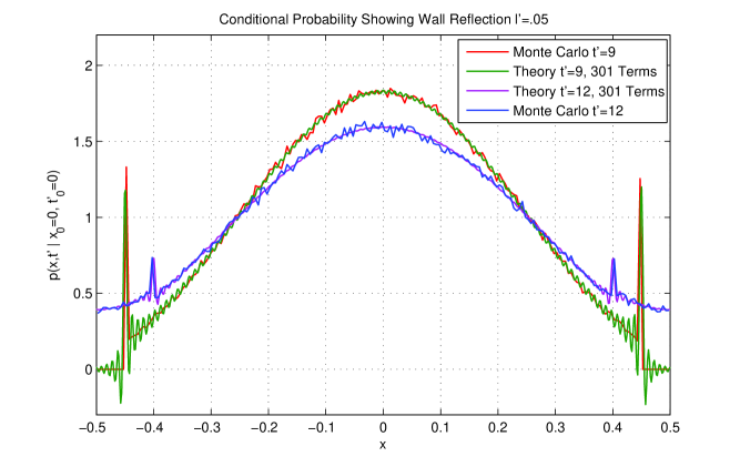
Figure 1: Conditional probability density with $x_{0}=0$ ,for the case $l_{c}=0.05,$ well into the diffusion limit, showing the agreement between the analytic result and the simulations for $t^{\prime}=9$ and $12$. The peaks representing the unscattered particles are clearly visible at these times as is the Gibbs phenomenon due to cutting off the high frequency terms.

The Gibbs phenomena is clearly seen in this plot. The Gibbs phenomenon arises due to the impossible task of representing an abrupt change with a finite series of continuous functions. In the finite sum the abrupt change can only be approximated by the fastest oscillating component, and in the limit of an infinite series the fastest frequency is infinite and the exact form is recovered.  However for purposes of plotting we cannot sum to infinite terms, and must accept the rapid oscillations, or smooth the rapid oscillations for a more pleasant and informative picture. To smooth the conditional density we take a running 4 point average. This is done for $4\times 500$ points across the region. Typically $20,001$ terms are summed prior to smoothing the functions but in this figure (fig. 2) we show the sum over only 301 terms for visibility.

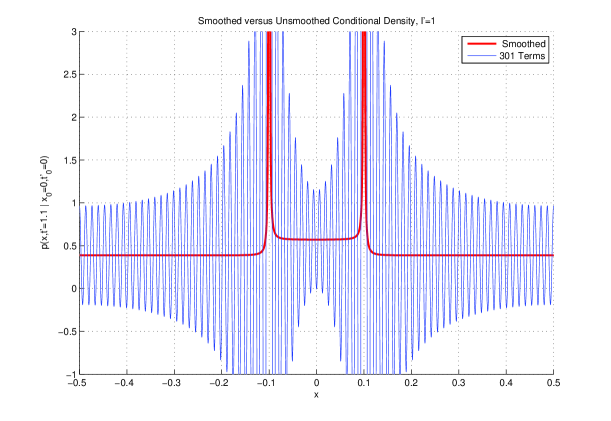
Figure 2: Conditional probability density with $x_{0}=0$ ,for the case $l_{c}=1,t^{\prime}=1.1$, approaching the ballistic limit. The particles have made one wall collision and have passed through each other $\left(v^{\prime}=l_{c}\right).$ Shown are a truncated sum $(N=301$ terms$)$ and the result of smoothing a sum with N=20,001.

The smoothing correctly shows the average of the rapid oscillations and gives a clearer picture.  The following (fig. 3) is a plot of the conditional density with $l^{\prime}=0.3.$ This is in the transition region. The peaks representing the initial trajectory of the particles are seen to be large for longer than a collision time. It is seen that the theory agrees extremely well with the Monte-Carlo simulations.

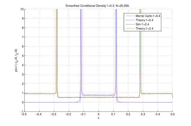
Figure 3: Conditional probability density with $x_{0}=0$ ,for the case $l_{c}=.3,t^{\prime}=0.4$ and $2.4.$ A wall collision has taken place between the two times shown. The build up of the wake of scattered particles is clearly visible.

In the earlier time the trajectories are moving away from each other, in the later time they have reflected against the wall and are moving toward each other. The initial trajectories are scattering at a slow enough rate to leave a uniform wake of probability behind them, the uniform probability is deposited in layers behind the traversing peaks. That is to say the rate of change of probability going from the initial trajectory into the wake is slow compared to the rate of crossing the cell. The wake appears uniform and the curve reminiscent of diffusion is not seen.  The following  (fig.4)is a plot for $l^{\prime}=1\vskip 12.0pt plus 4.0pt minus 4.0pt.$ More toward the ballistic region, however still somewhat in the transition region.

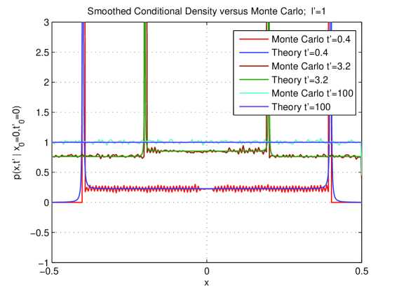
Figure 4: Conditional probability density with $x_{0}=0$ ,for the case $l_{c}=1,t^{\prime}=0.4,3.2$ and $100.$ By the later time the density is uniform and the unscattered peaks are gone,

This behavior is similar to the $l^{\prime}=0.3$ case. The wake of probability deposited behind the peaks is less, however after a long time the peaks can no longer be seen and a uniform distribution is found. The proposed theory is shown to agree very well with the Monte-Carlo simulations.

We see in general that as we are considering particles starting with velocities $\pm v$, there are 2 peaks, representing unscattered particles moving away from $x_{0}$ in opposite directions. The peaks are decaying in time while a ’wake’ of scattered particles builds up in the region behind them. The time development can be followed as the particles make multiple collisions with the walls. For short $\tau_{c}$ the wake morphs into the diffusion theory result, where the ’wake’ is position dependent, after some time. For the ballistic case of longer $\tau_{c}$, the wake does not develop any significant spatial dependence while the peaks decay with time. In all cases the wake behind the unscattered particles are larger than the wake ahead of them.

IV Calculation of Spectrum of Correlation functions.

Now, starting with (22) we can calculate the position correlation function according to (12) and then take the Fourier transform to obtain the spectrum. We can differentiate (22) with respect to $\tau$ to get the velocity position correlation function according to, Pap

$$R_{xv}\left(\tau\right)=-\frac{\partial}{\partial\tau}R_{xx}\left(\tau\right)$$ (27)

and a further differentiation will give the velocity autocorrelation function, Barab . We can calculate correlation functions involving quantities which vary arbitrarily with position. The results will be valid for short times and small distances allowing to consider fields varying over distances small compared to the collisional mean free path.

As it is usually the spectrum of the correlation function that is of interest we give here the Fourier transform of (22) that can then be integrated over arbitrary field distributions to give the desired spectrum.

$$G(x,x_{0},\omega) =\int_{0}^{\infty}p(x,\tau~{}|~{}x_{0},0)e^{i\omega\tau}d\tau$$ (28)

$$=\frac{1}{L}\left\{\sum_{n=even}\cos\left(\frac{n\pi x}{L}\right)\cos\left(\frac{n\pi x_{0}}{L}\right)+\sum_{n=odd}\sin\left(\frac{n\pi x}{L}\right)\sin\left(\frac{n\pi x_{0}}{L}\right)\right\}\times$$ (29)

$$\times\left\{Q_{2}\left(\omega\right)\left(1+\frac{1}{s_{n}}\right)+Q_{1}\left(\omega\right)\left(1-\frac{1}{s_{n}}\right)\right\}$$ (30)

where

$$Q_{1,2}\left(\omega\right)=\frac{\eta_{1,2}+i\omega}{\omega^{2}+\eta_{1,2}^{2}}$$ (31)

are the Fourier transforms of $e^{-\eta_{1,2}\tau},$ with $\eta_{1,2}$ given by (16). We see the results for the correlation functions will be given in terms of Fourier transforms of the arbitrary field variations, similar to the case with diffusion theory Clayt , Petu .

This will now be applied to the problem of an axion mediated interaction with the walls, Petu and to the problem of relaxation caused by a magnetic dipole impurity on the walls of the measuring cell, Heil .

V Derivation of the false electric dipole moment systematic error in a Linear Field with the Generalized Conditional Density.

In the case of a constant gradient across the bound region, the proposed conditional density should give the same phase shift as Swank . Using the equation (27)

$$\left\langle h_{x}\left(t-\tau\right)v_{x}(t)\right\rangle=\frac{\partial}{\partial\tau}\left\langle h_{x}(t)x(t+\tau)\right\rangle$$

Where the correlation of the field strength and position in terms of the conditional density for a linear gradient,

$$\left\langle h_{y}(t)y(t+\tau)\right\rangle=\int_{-\frac{L}{2}}^{\frac{L}{2}}dx_{0}G_{x}x_{0}~{}p(x_{0,}t)\int_{-\frac{L}{2}}^{\frac{L}{2}}x~{}p(x,t~{}|\;x_{0},t+\tau)~{}dx$$ (32)

Where $G_{x}$ is the strength of the linear gradient.

$$\left\langle h_{x}(t)x(t+\tau)\right\rangle=\frac{4L^{2}G_{x}}{\pi^{4}}e^{-\frac{\tau}{2\tau_{c}}}\sum_{n=odd}^{-\infty\rightarrow\infty}\frac{1}{n^{4}}\left\{\cosh\left(\frac{s_{n}}{2\tau_{c}}\tau\right)+\frac{1}{s_{n}}\sinh\left(\frac{s_{n}}{2\tau_{c}}\tau\right)\right\}$$ (33)

$$\left\langle h_{x}\left(t-\tau\right)v_{x}(t)\right\rangle=\frac{8L^{2}G_{x}}{\pi^{4}}\sum_{n=odd}^{-\infty\rightarrow\infty}\frac{\omega_{n}^{2}\tau_{c}}{n^{4}s_{n}}e^{-\frac{\tau}{2\tau_{c}}}\sinh\left(\frac{s_{n}\tau}{2\tau_{c}}\right)$$ (34)

We now write it in a form which only sums $n$ from $1~{}$to $\infty.$(we multiply by 2.)

$$h_{xv}(\tau)=\left\langle h_{x}\left(t-\tau\right)v_{x}(t)\right\rangle=\frac{16v^{2}\tau_{c}G_{x}}{\pi^{2}}\sum_{n=odd}^{1\rightarrow\infty}\frac{1}{n^{2}s_{n}}e^{-\frac{\tau}{2\tau_{c}}}\sinh\left(\frac{s_{n}\tau}{2\tau_{c}}\right)$$

To find the phase shift we take the cosine transform according to the prescription in (LamGo ) and (Barab ).

$$H_{xv}(\omega) =\int_{0}^{\infty}\cos(\omega_{o}\tau)h_{xv}\left(\tau\right)d\tau$$

$$H_{xv}\left(\omega\right) =\frac{8v^{2}G_{x}}{\pi^{2}}\sum_{n=odd}^{1\rightarrow\infty}\frac{1}{n^{2}}\frac{\left(\omega^{2}-\omega_{n}^{2}\right)}{\left(\omega^{2}-\omega_{n}^{2}\right)^{2}+\frac{\omega^{2}}{\tau_{c}^{2}}}$$

We notice that this field strength correlation spectrum gives the expected zero frequency value.

$$H_{xv}\left(\omega=0\right)=-G_{x}L_{x}^{2}\frac{8}{\pi^{4}}\sum_{n=odd}^{1\rightarrow\infty}\frac{1}{n^{4}}$$

We arrive at the expected phase shift found in (LamGo ).

$$\delta\omega(\omega_{0})=-\frac{\gamma^{2}E}{2c}H_{xv}(\omega_{0})$$

VI References

VII Appendix, considerations of wall reflections

We set $t_{0}=0.~{}$This can be thought of as the time for the RF pulse, where the conditional density is a delta function and the initial probability density is flat with value $\frac{1}{L}$. Now we consider a reflection from a single wall

$$p(x,t~{}|~{}x_{0})~{}=\delta\left(x0+vt-\frac{L}{2}-(\frac{L}{2}-x)\right)=\delta\left(x0+vt-L+x)\right)$$ (35)

The two terms should be summed for a complete description from $t=0$. Now say we are confined from -L/2 .. L/2. So we make a second wall reflection giving us an impulse at

$$p(x,t~{}|~{}x_{0})=\delta(x0+vt-2L-x)$$ (36)

and another wall

$$p(x,t~{}|~{}x_{0})=\delta\left(x_{0}+vt-3L+x)\right)$$ (37)

and another…

$$p(x,t~{}|~{}x_{0})=\delta(x_{0}+vt-4L-x)$$ (38)

More Generally

for $v>0$  and $x>x_{0}|_{t_{0}=0}$

$$p(x,t~{}|~{}x_{0},t_{0}=0)=\sum_{n=0}^{\infty}\delta(x_{0}+vt-2nL-x)+\sum_{n=0}^{\infty}\delta(x_{0}+vt-(2n+1)L+x)$$ (39)

and for $v>0|_{t=t_{0}}$ and $x<x_{0}|_{t_{0}=0}$

$$p(x,t~{}|~{}x_{0},0)=\sum_{n=0}^{\infty}\delta(x_{0}+vt-2nL-x)+\sum_{n=0}^{\infty}\delta(x_{0}+vt-(2n+1)L+x)$$ (40)

and for $v<0|_{t=t0}$ and $x>x_{0}|_{t_{0}=0}$

$$p(x,t~{}|~{}x_{0},0)=\sum_{n=0}^{\infty}\delta(x_{0}+vt+2nL+x)+\sum_{n=0}^{\infty}\delta(x_{0}+vt+(2n+1)L-x)$$ (41)

and for $v<0|_{t=t0}$ and $x<x_{0}|_{t_{0}=0}$

$$p(x,t~{}|~{}x_{0},0)=\sum_{n=0}^{\infty}\delta(x_{0}+vt+2nL+x)+\sum_{n=0}^{\infty}\delta(x_{0}+vt+(2n+1)L-x).$$ (42)

Now we make the assumption that at every $x_{0}$ there should be equal probability of a $+v$ and $-v.\$ Furthermore we can combine the $x<x_{0}|_{t_{0}=0}~{}$ and $x>x_{0}|_{t_{0}=0}~{}$initial conditions.

With that we have defined a conditional density for particles in one dimension with no gas scattering and purely specular wall reflections. We use the expansion of the delta function as:

$$\delta(x-x_{0}) =\frac{1}{L}\sum_{n=even}\cos\left(\frac{n\pi x}{L}\right)\cos\left(\frac{n\pi x_{0}}{L}\right)$$ (43)

$$+\frac{1}{L}\sum_{n=odd}\sin\left(\frac{n\pi x}{L}\right)\sin\left(\frac{n\pi x_{0}}{L}\right).$$

Where $n$ goes from $-\infty~{}~{}to~{}\infty$  with even/odd respectively for each sum.

References

• (1) A.G. Redfield, IBM Journal of Researcha dn Development, 1, 15 (1957)
• (2) C.P. Slichter, ”Principles of Magnetic Resonance”, Harper and Row, New York (1963)
• (3) D, McGregor Phys. Rev. A41, 2631 (1990)
• (4) A.L. Barabanov, R. Golub and S.K. Lamoreaux, Phys. Rev A74, 052115 (1996)
• (5) S.M. Clayton, arXiv:1012.1238
• (6) A.K. Petukhov et al, Physical Review Letters
• (7) J.M. Pendlebury et al, Phys. Rev. A70, 032102 (2004)
• (8) S.K. Lamoreaux and R. Golub, Phys. Rev. A71, 032104 (2005)
• (9) R. Golub, C.M. Swank, S.K. Lamoreaux, Β arXiv:0810.5378
• (10) R. Golub, R.M. Rohm and C.M. Swank, arXiv:1010.6266 and Phys. Rev., to be published.
• (11) A. Haji-Sheikh and J.V. Beck, Int. J. Heat ans Mass Transfer, 37, 2615, (1994)
• (12) P.M. Morse and H. Feshbach, ”Methods of Theoretical Physics”, McGraw Hill, New York, (1953)
• (13) Y.M. Ali and L.C, Zhang, Int. J. of Heat and Mass Transfer, 48, 2397 (2005) Y.M. Ali and L.C, Zhang, Int. J. of Heat and Mass Transfer, 48, 2741 (2005)
• (14) A. Haji-Sheikh, W.J. Minkowycz and E.M. Sparrow, J. Heat Transfer, 124, 307, (2002)
• (15) G. Chen, PRL 86, 2297 (2001)
• (16) D.D. Joseph and L. Preziosi, Rev. Mod. Phys. 61, 41 (1989) and 62, 375 (1990)
• (17) S. Goldstein, Quart. J. Mech. and Applied Math. IV, Pt. 2, 129, (1951)
• (18) P.A. Lemieux, M.U. Vera and D.J Durian, Phys. Rev. E57, 4498 (1998)
• (19) D.J. Durian and J. Rudnick, J. Opt. Soc. Am. A14, 235 (1997)
• (20) A. Papoulis, Probability, Random Variables and Stochastic Processes, McGraw-Hill, New York, (1965)
• (21) J. Schmiedeskamp, H.-J. Elmers, W. Heil et al, Eur. Phys J. D38, 445, (2006)