overview article: arxiv:1012.3982
Review of AdS/CFT Integrability, Chapter III.6:
Thermodynamic Bethe Ansatz
Zoltán Bajnok
Theoretical Physics Research Group of the
Hungarian Academy of Sciences,
H-1117 Pázmány s. 1/A, Budapest, Hungary
bajnok@elte.hu
![[Uncaptioned image]](/html/1012.3995/assets/x1.png)
Abstract:
The aim of the chapter is to introduce in a pedagogical manner the concept of Thermodynamic Bethe Ansatz designed to calculate the energy levels of finite volume integrable systems and to review how it is applied in the planar AdS/CFT setting.
Mathematics Subject Classification (2010):
81T30, 81T40, 81U15, 81U20
Keywords:
Thermodynamic Bethe Ansatz, planar AdS/CFT
1 Introduction
Thermodynamic Bethe Ansatz (TBA) is a method to calculate exactly the groundstate energy of an integrable quantum field theory in finite volume using its infinite volume scattering data [1]111The method has its origin in the work of Yang and Yang applied for spin chains and for the Bose gas with interaction [2].. The equations can be extended to excited states as well by analytical continuation [3, 4].
The idea of the TBA is to exploit that the Euclidean partition function is dominated for large imaginary times by the groundstate energy. Calculating the partition function in the doubly Wick rotated (mirror) theory the imaginary time becomes the physical size which is taken to be large. Since the large volume spectrum is under control, the partition function can be evaluated in the saddle point approximation which results in nonlinear integral equation for pseudo energies leading to an exact description of the ground state energy. Excited states on the complex (volume/coupling) plane are connected to the groundstate which enables one to derive nonlinear integral equations for excited states as well.
We start in Section 2 with a toy model containing one single particle with AdS dispersion relation and with scattering matrix which is not a function of the differences of the momenta. Although this is a fictitious system it helps to introduce conceptual notions and steps needed to explain the TBA which is, in analogy, used in Section 3 to present the results for planar AdS/CFT. Finally, we give a guide to the literature in Section 4 and list some open problems.
2 The concept of TBA: a toy model
The application of the TBA method to solve completely the finite volume spectral problem is standard by now and follows the following steps. First the scattering theory has to be solved in infinite volume by determining the scattering matrix from its generic properties such as symmetry, unitarity, crossing relation. The poles of the scattering matrix lying in the physical strip are related to bound-states. These bound-states have to be mapped and their scattering matrices have to be determined from the constituents’ scattering matrices. Then in the second step these scattering matrices can be used to describe the spectrum for large volume, which amounts to restrict the allowed particles’ momenta via phase shifts and periodicity, and use the dispersion relation to express the energy in terms of the quantized momenta. This method sums up all power like corrections in the inverse of the volume and provides an asymptotical spectrum. The very same asymptotic description of the mirror theory is also needed as it can be used to calculate the exponentially small finite energy corrections from the partition function. Evaluating the Euclidean partition function for large imaginary times (large mirror volumes) in the saddle point approximation provides integral equations describing the ground state energy exactly. Finally, these equations can be extended for excited states by analytical continuation. Now let us see how these steps are elaborated in the simplest setting.
Infinite volume characteristics of the model
We consider a toy model with one single particle type only. The dispersion relation is supposed to be the same as in the AdS/CFT correspondence 222The string tension is related to the ’t Hooft coupling as :
The sine function indicates lattice behavior and restricts the momentum as . The square root, however, has a relativistic origin. The theory is supposed to be integrable, thus multiparticle scattering matrices factorize into two particle scatterings. As relativistic invariance is not supposed the two particle S-matrix can depend separately on the two momenta and satisfies unitarity and crossing symmetry, which helps to fix it completely. We will not need its explicit form, but will suppose that in the particular case .
Infinite volume characteristics of the mirror model
The Euclidean version of the model is defined by analytically continuing in the time variable and considering space and imaginary time on an equal footing. The Euclidean theory so obtained can be considered as an analytical continuation of another theory, in which serves as the analytically continued time and is the space coordinate. The theory defined in terms of is called the mirror theory and its dispersion relation can be obtained by the same analytical continuation and which results in
Contrary to the original theory the mirror model is not of the lattice type as its momentum can take any real value As the scattering matrix is related via the reduction formula to the Euclidean correlator the mirror S-matrix is simply the analytical continuation of the original scattering matrix: .
Very large volume solution: asymptotic Bethe Ansatz for the model
Let us put particles in a large volume subject to periodic boundary condition. Integrability ensures that the particle number is conserved and the particles’ momenta are not changed in the consecutive scatterings. The leading effect of the finite volume is the momentum quantization constraint:
| (2.1) |
which is called the Bethe Yang equation or asymptotic Bethe Ansatz (ABA) and follows from the periodicity of the multiparticle wave function. Due to the sine function in the dispersion relation and the periodicity of consistency of (2.1) requires to take integer values only.
Bound-states of the theory are manifested in the ABA as complex string-like solutions. Indeed, if the scattering matrix has a pole for , then complex solutions are also allowed in (2.1). If we take very large with then the rhs. of (2.1) would go to which should be compensated by another complex momentum, say, such that exhibits a pole. The two particles with momenta and form a bound-state with momentum , energy and scattering matrix . In general complex solutions built up from more particles are also allowed and they usually form a string-like pattern. Their dispersion relation and scattering matrices can be calculated by extending the method above, which is called the S-matrix bootstrap.
Very large volume solution: ABA for the mirror model
In the mirror model the considerations go along the same line as in the original theory. If we denote the mirror volume by the ABA reads as
| (2.2) |
Since lives in a different analytical domain than its pole structure can be also different. If it exhibits poles also at the proper location the mirror theory has also bound-states. Once bound-states exist we can calculate their dispersion relation and scattering matrices from the bootstrap method. Suppose that the bound-states can be labeled with some charge , they have energy and their scattering matrix is . The generic ABA valid for all the excitations (also for bound-states) will be
| (2.3) |
Once these equations are solved the energy of the multiparticle state is
which describes the spectrum asymptotically for large volumes .
Groundstate TBA equation from the partition function
Let us come back to the original model and see how the exact groundstate energy can be determined in a finite volume from the Euclidean partition function. We exploit the fact that the imaginary time evolution for large times, , is dominated by the lowest energy state
where the ellipsis represents terms exponentially suppressed in The same partition function can be determined alternatively, using the time evolution of the mirror theory which is generated by the mirror Hamiltonian :
| original model | mirror model |
|---|---|
![[Uncaptioned image]](/html/1012.3995/assets/x2.png) |
![[Uncaptioned image]](/html/1012.3995/assets/x3.png) |
The relation between the original model and the mirror model is summarized in Table 1. In switching to the mirror model we ensure that the volume goes to infinity (and not the imaginary time) where the spectrum is controlled by the ABA (2.3).
In the large limit the sum in the partition function is dominated by finite density particle states. Introducing the density of the particles (and bound-states) in momentum space () the energy can be expressed as
where for later convenience we reparametrized the momentum as , momentum integrations go from to . The quantization condition comes from taking the logarithm of the mirror ABA
| (2.4) |
where labels the quantized momentum whose charge is . For a generic multiparticle state there are momenta which satisfy the same equation but which are not excited, not present in the system. They are called holes and their densities in the large volume limit is described by Clearly the densities of particles and holes are not independent they are connected by the thermodynamical limit of eq. (2.4) as
| (2.5) |
where the kernel is defined as
The particle density itself does not characterize properly the states we sum over in the partition function. Indeed in a given interval the occupied particles can be distributed different ways leading to an entropy factor in the sum. Since in the large particle number limit the factorials can be approximated with the Stirling formula the partition function will take the form
where the entropy factor is
One can slightly generalize the partition function by adding a chemical potential term to the energy where . For fermions we take , while for bosons . This extended partition function can be evaluated in the saddle point approximation. Taking into account the relation between and originating from the variation of (2.5) we obtain the minimizing equation in the so called pseudo energy as
Once the pseudo energies are determined the ground state energy in volume can be obtained as
| (2.6) |
The nonlinear integral equation which determines the pseudo energies is called the thermodynamic Bethe Ansatz (TBA) equation. Although it is not possible to solve it in general it provides an implicit exact description of the groundstate energy. This implicit solution is a starting point of a systematic large and small volume expansion and can be used to derive either functional relations for the pseudo energies or TBA equations for excited states by analytical continuation.
Excited states by analytical continuation
Here we start with bosonic theories without bound-states and suppose that by analytically continuing in some parameter (say in the volume) we can reach all excited states. The way how excited states appear can be understood by analyzing the energy expression (2.6) integrated by parts
Let us suppose that in the analytical continuation singularities of type appear. When we deform the contour their residue contributions give rise to
where we took into account the relation between the energy and the mirror momentum . Taking the same analytical continuation in the equation for the pseudo energy we obtain
Solving these equations iteratively for large we can recognize that the equations, which determine the positions of the singularities, coincide at leading order with the ABA equations (2.1). The subleading order calculation provides a universal formula for the leading finite size correction of multiparticle energy levels [5]. Alternatively for doing the analytical continuation one can think of the final result as choosing a different integration contour which surrounds the singularities, and when we take the integration contour back to the real axis we pick up the above residue contributions.
Finally we note that if we have more species (labeled by ) with diagonal scatterings (like in the previous subsection) then a singularity in results in the equations
whose solutions and have to be plugged into the energy formula
One has to be careful with such an analytical continuation in the presence of bound-states. Bound-states require pole singularities of the scattering matrices which usually cross the integration contour in the analytical continuation and result in extra source terms. See the Lee-Yang model in the relativistic case [3, 4] for example.
3 TBA for planar AdS/CFT
In this section we push forward the TBA program for planar AdS/CFT. The main difference compared to the previous discussion lies in the nondiagonal nature of the scattering matrix. There is a way, however, how we can profit from the previous diagonal results: the nondiagonal nature of any theory can be encoded into a diagonal theory but with auxiliary degrees of freedom. These auxiliary excitations do not contribute to the energy merely modifies the allowed momenta. Let us now follow the steps of Section 2.
3.1 Infinite volume characteristics of the model
The symmetry algebra of the theory has a factorized form: . The fundamental particle called magnon transforms in the bifundamental representation whose S-matrix has the structure
| (3.1) |
where the matrix part is fixed from its covariance under one copy of up to a scalar factor, which is determined from unitarity and crossing symmetry. The scattering matrix has simple poles corresponding to bound-states. There is an infinite tower of bound-states labeled by a positive integer charge . They transform under the tensor product of the atypical totally symmetric representations of the algebra and have dispersion relation
3.2 Infinite volume characteristics of the mirror model
As the mirror model is derived from the same Euclidean theory the fundamental particles’ scattering matrix is the analytical continuation of the scattering matrix (3.1). We are in a different analytical domain, however, and here different poles correspond to bound-states. These bound-states are also labeled by the charge but they transform under the atypical totally antisymmetric representations and have dispersion relation:
3.3 Very large volume solution: ABA for the model
If we put particles in a finite volume the momenta of the particles will be quantized. The multiparticle wave function has to be periodic in each argument, that is when a particle transported along the cylinder it scatters on all other particles before arriving back to its initial position. In a diagonal theory this results in (2.1). In a nondiagonal theory, however, the multiparticle transfer matrix has to be diagonalized. This can be achieved by introducing new type of (magnonic) particles with vanishing dispersion relations and considering the original problem in terms of them as a diagonal scattering theory.
Here we focus only on the charge sector of the theory. We have momentum carrying particles () which scatter on each other as 333The index in refers to the charge of the particle. This particle is a first member of an infinite series of bound-states labeled by . Similarly we will meet particles of type and .
where and represents the dressing phase. These particles are extended for each factor with two types of auxiliary particles (), whose parameters are labeled by and . The auxiliary particles have trivial dispersion relations (their energy and momentum are zero) and scatter with the fundamental, momentum carrying ones as
Furthermore, they scatter on each other as
where and we introduced a useful function . Any scattering matrix can be extended by unitarity to the opposite order of their particle types/arguments: .
In formulating the ABA equations for the full theory we have to take into account the two factors and that they commute. The ABA equation for the momentum carrying particles reads as
where is the number of fundamental and the number of type particles, while the index refers to the two factors. Since the two factors commute the ABA equations for the auxiliary particles with rapidities and can be written as
Not all solutions of the ABA equations correspond to single trace operators as the level matching/zero momentum condition has to be fulfilled . The theory contains also bound-states which can be determined from the singularity structure of the scattering matrices. Since from the TBA point of view only the bound-state spectrum of the mirror theory is relevant we will focus only on them.
3.4 Very large volume solution: ABA for the mirror model
In the case of the mirror theory the fundamental scattering matrix is the analytical continuation of the original one . As a result the ABA will be the analytical continuation, too
| (3.2) | |||||
| (3.3) | |||||
| (3.4) |
There are some differences compared to the original ABA. First the domain of is different compared to and the total mirror momentum does not need to vanish. Then, as we are in the mirror theory, the way how is expressed in terms of is also different: . Additionally, in the calculations of the ground state energy the sectors with antiperiodic fermions are relevant and this is manifested in a minus sign in the middle equation. The possible bound-states and their ABA equations are the subject of the next section. Let us note that usually in the literature instead of (3.4) its inverse is considered as this will lead to positive particle densities in the thermodynamic limit.
3.5 Exact groundstate energy: TBA
In this section we derive TBA integral equations for the groundstate energy in finite volume . We treat the theory as if it were diagonal with the scattering matrices specified above. First we analyze whether this “diagonal” theory has bound-states by analyzing the thermodynamic behavior of the equations and calculate the scattering matrices of the bound-states, the so called strings. They are special complex solutions of the ABA equations and they all contribute to the partition function which determines the ground state energy. Then we use the canonical procedure to derive coupled integral equations for the pseudo energies in a raw form, finally, using identities between the scattering matrices originating from the symmetry, we rewrite them in a simplified form and analyze simple excited states.
3.5.1 String hypothesis for the mirror model
The string hypothesis is similar to closing the S-matrix bootstrap program, that is to identify all particles (including bound-states) of the theory and to determine their scattering matrices. Let us premise that we will find bound-states of three infinite types for and also of a finite type particle with . They can be arranged in the two dimensional lattice shown in Figure 1. Let us see how they arise from the ABA equations.
In the following we put and all particle numbers large (keeping their ratio finite) and analyze the ABA one by one. Let us first note the reality properties of the equations. Unitarity of the mirror scattering matrix implies that the roots come in complex conjugated pairs or lie on the unit circle , similarly the roots come in complex conjugated pairs or are real.
particles
In looking for momentum bound-states we rewrite the scattering matrix in (3.2) as
where the rapidity is introduced as . As is very large complex values for with positive imaginary part are allowed. In this case the lhs. of (3.2) for diverges so there should be another say that goes to . If still has a positive imaginary part then by the same argument there should be another say which goes to . Applying this procedure we arrive at a string of roots or shortly where . (Clearly the string is the original particle itself.) The scattering of the -string with any other particle of type , label and rapidity is
Although naively the scattering matrices seem to depend on the parameters and such a way the bound-state scattering matrix depends on its constituents, this is not the case when we take into account the contributions of the dressing phase as was shown in [6].
The auxiliary particles exist for both ) factors. Here we focus only on one of them and omit to write out its index.
particles
Let us analyze (3.3). If we suppose that the number of momentum carrying particles goes to infinity then
| (3.5) |
In the middle case roots lying on the unit circle are allowed. As the scattering matrix has a difference form in the variable we might use the parameter instead of . The inverse of the relation, however, is not unique. Defining with the branch cuts running from to we can describe any with for . Clearly describes the other case and in the scattering matrices which depends on , and not on , we have to specify which root is taken. As a consequence we have two types of particles with and the scattering matrices split as .
particles
If in (3.5) then the rhs. of (3.3) goes to zero which has to be compensated by a root which goes to But then taking the ABA for means that the rhs. of (3.4) will diverge which has to be compensated by a root . If the corresponding satisfies then (3.3) is consistent with (3.5) and reality requires , . The three roots and and form an string which we denote by . In the case when then we have to repeat the same arguments for leading to and and so on. Finally we arrive at the notion of a string. It consists of particles with and particles with synchronized parameters and for . The composite scattering matrix of the particle with all other particles is simply the product of the scatterings of its each individual constituents
particles
Suppose we have a large number of particles and that has a positive imaginary part. Then the first factor of the rhs. of (3.4) will go to zero which has to be compensated by a root . If then we obtain a string. In the opposite case we repeat to previous argumentation leading to an string . Clearly a single is just a string. The scattering of the string with any other particle is
Scattering matrices
Summarizing, the mirror AdS theory in the thermodynamic limit could be replaced by a diagonal theory having constituents of infinite type and index for and also of finite type particles with . See also Figure 1.
For the readers convenience we summarize the scattering matrices in Table 2. The scattering matrices are unitary and their explicit forms are
where and we reparametrized the momentum carrying particles in terms of the rapidity via the function . Recall also that . The other matrix elements are
The ABA equations then have a generic form
where . can be any type of but only the particles have nonvanishing energy and momentum . The parameter denotes the fermion number. We also indicated the contributions of the two factors. The energy of such a multiparticle state having of particles is
Let us note that the ABA equations for the auxiliary particles can be inverted without changing their physical meaning. Taking the inverse of (3.4) is equivalent to redefining simultaneously the scattering matrices and . Actually these are the equations used in the literature as they give positive particle densities in the thermodynamic limit.
3.5.2 Raw TBA equations
Suppose now that we would like to describe the groundstate energy in the AdS system in volume . In doing so we follow the steps presented in Section 2 to evaluate the partition function for large mirror sizes. We introduce densities of particles (strings) for and for and the analogous densities of holes They are restricted via the logarithm of the ABA which contains the logarithmic derivatives of the scattering matrices
Clearly as the scattering matrices are not of the difference type. (Keeping in mind how we obtained the string solutions the densities are naturally ordered .) Then we introduce the entropy factors for the densities, chemical potential for fermions and calculate the saddle point of the functional integral. This results in integral equations for the pseudo energies as follows
where in the contributions of the and we have to sum for the contributions of the two ) factors (which we omitted to write out). The remaining equations are valid separately for the two factors separately:
Once these equations are solved the groundstate energy can be obtained as
Finally we note that we replaced the magnonic ABA for the particle type with its inverse and made the corresponding change in the scattering matrices to ensure the positivity of the magnonic densities . It effectively changed the sign of the related kernels.
3.5.3 Simplified TBA equations and Y-system
In this subsection using identities among the TBA kernels we bring the equations in to a universal local form. This means that pseudo energies can be drawn in a two dimensional lattice, such that only neighboring sites couple to each other with the following universal kernel
| (3.6) |
where and . To simplify the notation let us introduce the following functions
Clearly we have two copies for . (To conform with the literature we inverted the ABA equations for and ). Acting with the operator (3.6) on these inverted TBA equations and using kernel identities like we arrive at their simplified, universal form
where in the convolution we integrate over the interval only. The other equations do not behave so nicely.
where vanishes on the interval whose explicit form can be found in [7]. The equation for the particles are simpler in the original form
These equations for are not in a local form. However, acting with the inverse of they can be brought into such form. The operator acts as and involves the analytical continuation of the functions. It has a large null space, thus when acting on the equation information is lost:
The advantage of defining in the above manner is that it uses the analytically continued values of the functions on the rapidity torus only. If we continue them across the cuts by using then the term disappears, but the functions have to be extended to an infinite genus Riemann surface. On this surface the Y-system has the universal form
| (3.7) |
where the indices live on a two dimensional integral lattice. In our situation the identification can be drawn on Figure 1, which explicitly reads as , , , and where and .

3.5.4 Excited states by analytical continuation
Here we focus on the TBA equations for excited states in the sector for small coupling. This sector contains particles of type only and have ABA:
These equations are asymptotic only and the exact system of TBA equations is required to describe the energy of the multiparticle state exactly. As the vacuum is a BPS state it has vanishing energy and its analytical continuation cannot describe excited states. Alternatively we choose an integration contour, such that when it is taken back to the real axis the residue of a singularity of the form is picked up resulting in additional source terms in the raw equations as:
Once the new system of TBA equations are solved the pseudo energies have to be plugged into the energy formula:
to obtain the energy of the multiparticle system.
We can rewrite the TBA equations in terms of the functions into their simplified form. They satisfy the same -system relations (3.7) but with a different asymptotical behavior. There is a systematical asymptotical expansion of the -system, which reproduces both the ABA and the leading Lüscher correction of these multiparticle states. This is valid for weak coupling (or large sizes) and it is very nontrivial to follow the analytical behavior of the functions as one increases the coupling. The ABA solution itself suggests, that additional singularities could appear and then the TBA equations have to be modified by additional source terms. These source terms ensure the analytical behavior of the energy around these singular points.
4 Guide to the literature
Here we list the representative papers where the various parts of the TBA program were developed.
The idea that the TBA program can be applied in the planar AdS/CFT setting was presented in [9]. The infinite volume scattering description of theory can be found in chapters [10, 11]. The ABA equations for the planar AdS/CFT model was conjectured in [12] (and thoroughly discussed in chapters [13, 14]), while the analogous ABA for the mirror model was described in [15]. As the color structure ( of the scattering matrix is the same as that of the Hubbard model, the Hubbard TBA solution can be adopted [16]. This results in the string hypothesis which was formulated explicitly in [17]. The standard procedure leads to raw TBA equations, which were developed in [19, 18, 20]. The simplified form of the TBA equations was presented in [7] and the Y-system relations, presented previously in [21], were derived in [19, 18, 20]. In doing this the analytical properties of the dressing phase [6, 20, 22] had to be investigated. In the AdS/CFT context the volume of the integrable system has to be an integer, which can be seen also on the groundstate TBA [23].
Although we obtained the Y-system from the ground-state TBA equations, in principle, it follows from the hidden symmetry of the model. An independent alternative approach based on this symmetry is the subject of the next Chapter in this volume [24].
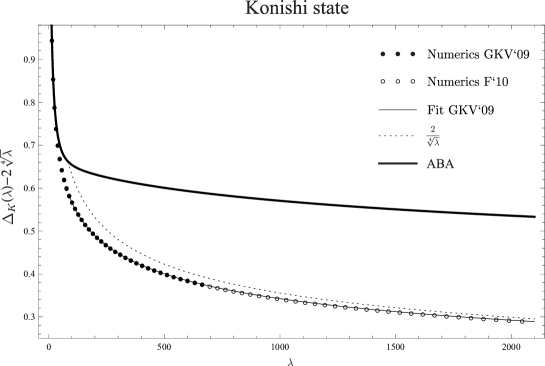
The Y-system plays a crucial role in describing excited states. As it is related to the symmetry of the model [24, 25, 26] it is the same for each state. What makes the difference is the asymptotical and analytical behavior of the Y-functions. The analytical properties of the Y-functions was thoroughly analyzed in [19, 28, 23, 8]. Based on the solution of the Y-system of the model [27] the authors of [21] identified the large volume solution in terms of the transfer matrices of the ABA [14]. This helps to derive excited states TBA equations for the sector, which was done in [20, 28]. The excited state TBA equations provide an exact description of the given state and they were used in the Konishi case, [29, 30], to analyze numerically the behavior of the energy for large coupling. The results are summarized in Figure 2444We thank the authors of [31] for borrowing their figure., see also [31]. It was further shown in [28] how to modify these excited state TBA equations if a singularity appears in the analytical continuation in .
The weak coupling limit of the Y-system equations can be compared to the ABA [14] and Lüscher type correction [32]. The leading order behavior is built in the asymptotic solution [21] of the Y-function, but the next to leading one provides a stringent test of the excited states TBA equations, which was performed numerically for the Konishi operator in [33] and analytically at next to leading order in [34]. Later this analytical calculation was extended to describe the next to leading order Lüscher correction of generic twist two states [35] in [36].
The strong coupling limit of the -system for a finite density of string particles was analyzed in [37], where a complete agreement with the one loop string energies including all exponential finite size corrections has been found. The functional -system equations were encoded into simpler functions in [38, 25, 31].
| This review | AF | BFT | GKKV | |
|---|---|---|---|---|
Let us mention, how our TBA equations are related to those in the literature. We summarized the relation between the various conventions for half of the Y-system in Table 2 as the other half is trivially related, see also [8]. Under this replacement our simplified equations are equivalent to AF [7], while the raw equations to BFT [18], except for the chemical potentials of [18]. In comparing to GKKV [20] the indentification is not enough. Comparing our kernel to the one in [20] we observe a slight difference. This is irrelevant, however, for excited states satisfying the level matching/zero momentum condition 555We thank the authors of [20] for pointing out this. .
The correspondence has a brother theory, the duality [39], where the TBA program has been developed in an analogous way. The ABA together with the string hypothesis of the mirror theory lead to ground state TBA equations and Y-system relations in [40, 41] and extend the previously conjectured Y-system proposal of [21]. This program is further elaborated in [41] by additionally determining excited states TBA equations and comparing them to the asymptotic solution of the Y functions [21] and to the quasi classical string spectrum.
Finally, let us list some open problems.
There are two disagreeing string theory calculations ([42] and [43]) for the anomalous dimension of the Konishi state. Additionally, the numerical solution of the TBA equations for large couplings [29, 30] provides a third result, and calls for improvements both the string theory and the TBA sides. On the string theory side it could be a pure spinor calculation, while on the TBA side one should analyze the analytical behavior of the Y-system and check whether, with increasing , a singularity of type indeed appears, as the asymptotic solution suggests [28]. In principle the effect of such singularities is to make the coupling dependence of the energies analytical, but it has to be established concretely.
The anomalous dimensions of twist operators in the planar limit can be described by integral equations derived directly from the ABA [44]. It would be nice to see, how the exact excited TBA equations reduce to these equations in the large spin limit.
The analytical comparision of the excited state TBA equations to the next to leading order Lüscher corrections [34, 36] tested explicitly only the part of the Y-system. A next to next to leading order analysis could test the part as well.
The excited states TBA equations are coupled nonlinear integral equations for infinite unknowns. An ideal system of equations should contain finite unknowns only, and could be developed in analogy to [27, 45] by exploiting the result of [38, 25, 31].
Acknowledgments
We thank G. Arutyunov, N. Beisert, D. Fioravanti, S. Frolov, N. Gromov, A. Hegedus, V. Kazakov, R. Suzuki and R. Tateo for useful comments on the manuscript. The work was supported by a Bolyai Scholarship, and by OTKA K81461.
Note added in proof
After this review chapter was finished three string theory calculations based on different methods determined the strong coupling expansion of the anomalous dimension of the Konishi operator [46, 47, 48]. All agreed with each other and with the strong coupling expansion of the TBA equation [29, 30]. This gives a strong support not only for the correctness of the TBA equations but also for the integrability approach to planar AdS/CFT.
References
- [1] A. B. Zamolodchikov, “Thermodynamic Bethe Ansatz in relativistic models. Scaling three state Potts and Lee-Yang models”, Nucl. Phys. B342, 695 (1990).
- [2] C.-N. Yang and C. P. Yang, “Thermodynamics of a one-dimensional system of bosons with repulsive delta-function interaction”, J. Math. Phys. 10, 1115 (1969).
- [3] P. Dorey and R. Tateo, “Excited states by analytic continuation of TBA equations”, Nucl. Phys. B482, 639 (1996), hep-th/9607167.
- [4] P. Dorey and R. Tateo, “Excited states in some simple perturbed conformal field theories”, Nucl. Phys. B515, 575 (1998), hep-th/9706140.
- [5] Z. Bajnok, A. Hegedus, R. A. Janik and T. Lukowski, “Five loop Konishi from AdS/CFT”, arxiv:0906.4062.
- [6] G. Arutyunov and S. Frolov, “The Dressing Factor and Crossing Equations”, arxiv:0904.4575.
- [7] G. Arutyunov and S. Frolov, “Simplified TBA equations of the AdS5 S5 mirror model”, arxiv:0907.2647.
- [8] A. Cavaglia, D. Fioravanti and R. Tateo, “Extended Y-system for the correspondence”, arxiv:1005.3016.
- [9] J. Ambjorn, R. A. Janik and C. Kristjansen, “Wrapping interactions and a new source of corrections to the spin-chain / string duality”, Nucl. Phys. B736, 288 (2006), hep-th/0510171.
- [10] C. Ahn and R. Nepomechie, “Review of AdS/CFT Integrability, Chapter III.2: Exact world-sheet S-matrix”, arxiv:1012.3991.
- [11] P. Vieira and D. Volin, “Review of AdS/CFT Integrability, Chapter III.3: The dressing factor”, arxiv:1012.3992.
- [12] N. Beisert and M. Staudacher, “Long-range PSU(2,24) Bethe ansaetze for gauge theory and strings”, Nucl. Phys. B727, 1 (2005), hep-th/0504190.
- [13] A. Rej, “Review of AdS/CFT Integrability, Chapter I.3: Long-range spin chains”, arxiv:1012.3985.
- [14] M. Staudacher, “Review of AdS/CFT Integrability, Chapter III.1: Bethe Ansätze and the R-Matrix Formalism”, arxiv:1012.3990.
- [15] G. Arutyunov and S. Frolov, “On String S-matrix, Bound States and TBA”, JHEP 0712, 024 (2007), arxiv:0710.1568.
- [16] F. H. L. Essler, H. Frahm, F. Goehmann, A. Kluemper and V. E. Korepin, “The One-Dimensional Hubbard Model, Cambridge University Press”.
- [17] G. Arutyunov and S. Frolov, “String hypothesis for the AdS5 S5 mirror”, JHEP 0903, 152 (2009), arxiv:0901.1417.
- [18] D. Bombardelli, D. Fioravanti and R. Tateo, “Thermodynamic Bethe Ansatz for planar AdS/CFT: a proposal”, arxiv:0902.3930.
- [19] G. Arutyunov and S. Frolov, “Thermodynamic Bethe Ansatz for the AdS5 S5 Mirror Model”, JHEP 0905, 068 (2009), arxiv:0903.0141.
- [20] N. Gromov, V. Kazakov, A. Kozak and P. Vieira, “Integrability for the Full Spectrum of Planar AdS/CFT II”, arxiv:0902.4458.
- [21] N. Gromov, V. Kazakov and P. Vieira, “Integrability for the Full Spectrum of Planar AdS/CFT”, arxiv:0901.3753.
- [22] D. Volin, “Minimal solution of the AdS/CFT crossing equation”, arxiv:0904.4929.
- [23] S. Frolov and R. Suzuki, “Temperature quantization from the TBA equations”, Phys. Lett. B679, 60 (2009), arxiv:0906.0499.
- [24] V. Kazakov and N. Gromov, “Review of AdS/CFT Integrability, Chapter III.7: Hirota Dynamics for Quantum Integrability”, arxiv:1012.3996.
- [25] N. Gromov, V. Kazakov and Z. Tsuboi, “PSU(2,2—4) Character of Quasiclassical AdS/CFT”, JHEP 1007, 097 (2010), arxiv:1002.3981.
- [26] D. Volin, “String hypothesis for gl(n—m) spin chains: a particle/hole democracy”, arxiv:1012.3454.
- [27] N. Gromov, V. Kazakov and P. Vieira, “Finite Volume Spectrum of 2D Field Theories from Hirota Dynamics”, arxiv:0812.5091.
- [28] G. Arutyunov, S. Frolov and R. Suzuki, “Exploring the mirror TBA”, arxiv:0911.2224.
- [29] N. Gromov, V. Kazakov and P. Vieira, “Exact AdS/CFT spectrum: Konishi dimension at any coupling”, arxiv:0906.4240.
- [30] S. Frolov, “Konishi operator at intermediate coupling”, arxiv:1006.5032.
- [31] N. Gromov, V. Kazakov, S. Leurent and Z. Tsuboi, “Wronskian Solution for AdS/CFT Y-system”, arxiv:1010.2720.
- [32] R. Janik, “Review of AdS/CFT Integrability, Chapter III.5: Lüscher corrections”, arxiv:1012.3994.
- [33] G. Arutyunov, S. Frolov and R. Suzuki, “Five-loop Konishi from the Mirror TBA”, arxiv:1002.1711.
- [34] J. Balog and A. Hegedus, “5-loop Konishi from linearized TBA and the XXX magnet”, arxiv:1002.4142.
- [35] T. Lukowski, A. Rej and V. N. Velizhanin, “Five-Loop Anomalous Dimension of Twist-Two Operators”, arxiv:0912.1624.
- [36] J. Balog and A. Hegedus, “The Bajnok-Janik formula and wrapping corrections”, arxiv:1003.4303.
- [37] N. Gromov, “Y-system and Quasi-Classical Strings”, arxiv:0910.3608.
- [38] A. Hegedus, “Discrete Hirota dynamics for AdS/CFT”, arxiv:0906.2546.
- [39] T. Klose, “Review of AdS/CFT Integrability, Chapter IV.3: = 6 Chern-Simons and Strings on ”, arxiv:1012.3999.
- [40] D. Bombardelli, D. Fioravanti and R. Tateo, “TBA and Y-system for planar ”, Nucl. Phys. B834, 543 (2010), arxiv:0912.4715.
- [41] N. Gromov and F. Levkovich-Maslyuk, “Y-system, TBA and Quasi-Classical Strings in AdS4 x CP3”, JHEP 1006, 088 (2010), arxiv:0912.4911.
- [42] G. Arutyunov and S. Frolov, “Uniform light-cone gauge for strings in AdS5 S5: Solving su(11) sector”, JHEP 0601, 055 (2006), hep-th/0510208.
- [43] R. Roiban and A. A. Tseytlin, “Quantum strings in AdS5 S5: strong-coupling corrections to dimension of Konishi operator”, arxiv:0906.4294.
- [44] L. Freyhult, “Review of AdS/CFT Integrability, Chapter III.4: Twist states and the cusp anomalous dimension”, arxiv:1012.3993.
- [45] V. Kazakov and S. Leurent, “Finite Size Spectrum of SU(N) Principal Chiral Field from Discrete Hirota Dynamics”, arxiv:1007.1770.
- [46] N. Gromov, D. Serban, I. Shenderovich and D. Volin, “Quantum folded string and integrability: from finite size effects to Konishi dimension”, arXiv:1102.1040.
- [47] R. Roiban and A. A. Tseytlin, “Semiclassical string computation of strong-coupling corrections to dimensions of operators in Konishi multiplet”, arXiv:1102.1209.
- [48] B. C. Vallilo and L. Mazzucato, “The Konishi multiplet at strong coupling”, arXiv:1102.1219.