Imperial-TP-AT-2010-05,
arxiv:1012.3986
overview article: arxiv:1012.3982
Review of AdS/CFT Integrability, Chapter II.1:
Classical string solutions
A.A. Tseytlin***Also at Lebedev Institute, Moscow.
Blackett Laboratory, Imperial College London, SW7 2AZ, U.K.
tseytlin@imperial.ac.uk
![[Uncaptioned image]](/html/1012.3986/assets/x1.png)
Abstract:
We review basic examples of classical string solutions in . We concentrate on simplest rigid closed string solutions of circular or folded type described by integrable 1-d Neumann system but mention also various generalizations and related open-string solutions.
1 Introduction
space plays a special role in superstring theory [4]. This space (supported by a 5-form flux) is one of the three maximally supersymmetric “vacua” of type IIB 10-d supergravity [5], along with its limits – the flat Minkowski space and the plane-wave background [6]. It appears as a “near-horizon” region of the solitonic D3-brane background [7]; that explains its central role in the AdS/CFT duality [8] (see [9] for a review). The duality states that certain “observables” in supersymmetric 4-d gauge theory have direct counterparts in the type IIB superstring theory in space, and vice versa.
The type IIB superstring theory in a curved space with a 5-form Ramond-Ramond (RR) background is defined by the Green-Schwarz [10] action ()
| (1.1) | |||
| (1.2) |
Here () are the bosonic string coordinates, () are two Majorana-Weyl spinor fields, () is an independent 2-d metric, are projections of the 10-d Dirac matrices, , is the vielbein of the target space metric, . is antisymmetric 2-d tensor and diag. is the projection of the 10-d covariant derivative . The latter is given by , where is the Lorentz connection and is the RR 5-form field. Here and should be related so that the 2-d Weyl and kappa-symmetry anomalies cancel.
In the case of the background the explicit form of the superstring action can be found using the supercoset construction [11]. The group of super-isometries (Killing vectors and Killing spinors or solutions of ) of this background is , i.e. the same as super-extension of the 4-d conformal group . Using that and the superstring action can be constructed in terms of the components of current restricted to the coset (see [12] for details).
Since the metric of has direct product structure, the bosonic part of the action (1.1) is a sum of the actions for the and sigma models. The two sets of bosons are coupled through their interaction with the fermions. The latter fact is crucial for the UV finiteness of the superstring model [11, 13, 14] (see also [15]).
Below we shall consider classical bosonic solutions of the string action. The study of classical string solutions and their semiclassical quantization initiated in [16, 17, 18, 19] is an important tool for investigating the structure of the AdS/CFT correspondence (for reviews see, e.g., [20, 21, 22, 23]). The AdS energy of a closed string solution expressed in terms of other conserved charges and string tension gives the strong coupling limit of the scaling dimension of the corresponding gauge-theory operator. Classical solutions for open strings ending at the boundary of describe the strong coupling limit of the associated Wilson loops and gluon scattering amplitudes (see [24] and [25, 26, 27]).
Coset space sigma models are known to be classically integrable [28, 29] and this integrability extends [30] also to the full kappa-invariant superstring action. The integrability allows one to describe, in particular, large class of (finite gap [31]) classical string solutions in terms of the associated spectral curve [32, 33] (see [34]).
This description is, however, formal and obscures somewhat the physical interpretation of the solutions. It is very useful to complement it with a study of specific examples of solutions that can be constructed directly from the sigma model equations of motion by starting with certain natural ansatze. This will be our aim below.
We shall mostly concentrate on the simplest spinning “rigid” closed string solutions for which the shape of the string does not change with time (extra oscillations increase the energy for given spins). We shall consider several types of solutions and their limits that reveal different patterns of dependence of the energy on the string tension and the spins. This provides an important information about the strong ‘t Hooft coupling limit of the corresponding gauge theory anomalous dimensions and thus aids one in understanding the underlying description of the string/gauge theory spectrum valid for all values of the string tension or ‘t Hooft coupling.
2 Bosonic string in
At the classical level (with fermion fields vanishing) the and parts of the string action are still effectively coupled through their interaction with 2-d metric . If one solves for one gets a non-linear Nambu-Goto type action containing interactions between the and coordinates. In the conformal gauge the classical equations for the and parts are decoupled, but there is a constraint on their initial data from the equation for , i.e. that the 2-d stress tensor should vanish (the Virasoro conditions). We shall study the corresponding solutions below but let us start with the definition of the space and the explicit form of the bosonic string action.
2.1 space
Just like the -dimensional sphere can be represented as a surface in
| (2.1) |
the dimensional anti - de Sitter space can be represented as a hyperboloid (a constant negative curvature quadric)
| (2.2) |
in with the metric
| (2.3) |
We set the radius of the sphere and the hyperboloid to 1. In what follows we will be interested in the case of .
It is often useful to solve (2.2),(2.1) by choosing an explicit parametrization of and in terms of 5+5 independent “global” coordinates
| (2.4) | |||||
Then the corresponding metrics are
| (2.5) | |||
| (2.6) |
and they are obviously related by an analytic continuation.
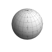
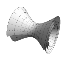
Note that choosing and (and standard periodicities for the angles ) already covers the hyperboloid once. Near “the center” the metric is that of while near its boundary it is that of . To avoid closed time-like curves and to relate the corresponding theory to gauge theory in it is standard to decompactify the direction, i.e. to assume . Thus in all discussions of AdS/CFT and in what follows by we shall understand its universal cover (in particular, we will ignore the possibility of string winding in global AdS time direction). In the case of plotted as a hyperboloid in that corresponds to going around the circular dimension infinite number of times or “cutting it open”. We present images of and of a universal cover of in Figure 1.†††We thank N. Beisert for sending us these figures. Another useful image of the universal cover of the space is a body of 2-cylinder with as a boundary and as a radial coordinate.
Let us mention also another choice of coordinates – the Poincaré coordinates – that cover only part of (for more details see, e.g., [9]):
| (2.7) |
Here () parametrizes the 3-sphere in (2.5): . Then the metric (2.5) takes the form ()
| (2.8) |
The full metric may be written also in the conformally-flat form as
| (2.9) |
where . The Poincaré coordinates are useful for the discussion of solutions representing open strings ending at the AdS boundary (see [25, 26, 27]).
2.2 String action, equations of motion and conserved angular momenta
The bosonic part of the action (1.1) in the conformal gauge is
| (2.10) |
where ( corresponds to ‘t Hooft coupling on the =4 super Yang-Mills side), is the (same) radius of and and
| (2.11) |
Here , and , are the embedding coordinates of with the Euclidean metric in and of with in , respectively (). and are the Lagrange multipliers imposing the two hypersurface conditions. The classical equations for (2.10) are
| (2.12) | |||
| (2.13) |
The action (2.10) is to be supplemented with the conformal gauge constraints
| (2.14) |
We will be interested in the closed string solutions with the world sheet as a cylinder, i.e. will impose the periodicity conditions
| (2.15) |
The action (2.10) is invariant under the and rotations with the conserved (on-shell) charges
| (2.16) |
There is a natural choice of the 3+3 Cartan generators of corresponding to the 3+3 linear isometries of the metric (2.5),(2.6), i.e. to the translations in the time , in the 2 angles and the 3 angles :
| (2.17) | |||
| (2.18) |
2.3 Classical solutions: geodesics
We will be interested in classical solutions that have finite values of the AdS energy and the spins (). The Virasoro condition will give a relation between the 6 charges in (2.17),(2.18) allowing one to express the energy in terms of the other 5, i.e. . Here stands for other (hidden) conserved charges, like “topological” numbers determining particular shape of the string (e.g., number of folds, spikes, winding numbers, etc).‡‡‡A simple example of an infinite-energy solution is an infinitely stretched string in described (in conformal gauge) by , , i.e. . It is formally periodic if . In the Poincare patch the corresponding solution is .
For a solution to have a consistent semiclassical interpretation, it should correspond to a state of a quantum Hamiltonian which carries the same quantum numbers (and should thus be associated to a particular SYM operator with definite scaling dimension). It should represent a “highest-weight” state of a symmetry algebra, i.e. all other non-Cartan (non-commuting) components of the symmetry generators (2.16) should vanish; other members of the multiplet can be obtained by applying rotations to a “highest-weight” solution.§§§For a discussion of the relation of the above charges to the standard conformal group generators in the boundary theory and a relation between representations labelled by the AdS energy and the dilatation operator see [21] and refs. there.
Let us start with point-like strings, for which in (2.12)–(2.14), i.e. with massless geodesics in . Then (as follows directly from (2.12),(2.13)) and (2.14) implies that . The generic massless geodesic in can be of two “irreducible” types (up to a global transformation): (i) massless geodesic that stays entirely within ; (ii) a geodesic that runs along the time direction in and wraps a big circle of . In the latter case the angular motion in provides an effective mass to a particle in , i.e. the corresponding geodesic in is a massive one,
| (2.19) |
The only non-vanishing integrals of motion are , representing the energy and the spin of this BPS state, corresponding to the BMN “vacuum” operator tr in the SYM theory [16] (see also [15]).
The solution for a massless geodesic in is a straight line in , with The angular momentum tensor in (2.16) is . It always has non-vanishing non-Cartan components [21], e.g., if we get . This geodesic thus does not represent a “highest-weight” semiclassical state. In terms of Poincare coordinates (2.8) the massless geodesic is represented by , i.e. it runs parallel to the boundary (reaching the boundary at spatial infinity where Poincare patch ends – that follows from its description in global coordinates).
Below we shall consider examples of extended (-dependent) solitonic string solutions of the equations (2.12),(2.13) subject to the constraints (2.14),(2.15) that have finite AdS energy and spins. The aim will be to find the expression for the energy in terms of other charges.¶¶¶Early discussions of semiclassical strings in de Sitter and Anti de Sitter spaces appeared, e.g., in [35, 36]. The fact that in AdS space the string mass scales linearly with large quantum numbers (as opposed to square root Regge relation in flat space) was first observed in [36]. In general, a string all points of which can move fast in will admit a “fast string” (BMN-type) limit in which will have an analytic dependence on the square of string tension or on when expressed in terms of and and expanded in large total spin of [18, 19]. At the same time, the energy of a string whose center is at rest or which moves only within the will depend explicitly on (i.e. will be non-analytic in ) [17, 19, 43].
3 Simplest rigid string solutions
Here we shall consider few simple explicit closed-string solutions of the non-linear equations (2.12),(2.13) which are “rigid”, i.e. for which the shape of the string does not change with time. These may be interpreted as examples of non-topological solitons of the conformal-gauge string sigma model (2.10) on a 2-d cylinder .
3.1 Examples of string solutions in flat space
Let us start with recalling several examples of string solutions in flat space. The flat-space string action and equations of motion in the conformal gauge are (, , )
| (3.1) |
The general solution of free equations subject to the closed string periodicity condition is parametrized by constants, which are constrained by the Virasoro conditions. Simple explicit solutions representing semiclassical (coherent) states corresponding to particular quantum states in the string spectrum have only finite number of the Fourier modes excited. The Virasoro condition then implies a relation between the energy of the string and its linear momenta, spins, oscillation numbers, etc. Some explicit examples are:
Folded string rotating on a plane:
| (3.2) | |||
| (3.3) |
Spiky string rotating on a plane:
| (3.4) | |||
| (3.5) |
Here is the number of spikes, i.e. is the case of the folded string.∥∥∥The relation between (3.4) and (3.2) for involves .
Circular string rotating in two orthogonal planes of :
| (3.6) | |||
| (3.7) |
Here are the values of the orbital momentum.
Circular string pulsating in one plane:
| (3.8) | |||
| (3.9) |
Here is the oscillation number (an adiabatic invariant). This solution is formally not rigid but is very similar – the shape of the string remains circular, only its radius changes with time. An example of a non-rigid solution is a “kinky string” [37] for which the string has a shape of a quadrangle at the initial moment in time, then shrinks to diagonal due to the tension, then expands back, etc.
3.2 Circular rotating strings: rational solutions
A simple subclass of “rational” solutions of the equations (2.12),(2.13) is found by assuming that [19, 38]. In this case and are given by simple trigonometric solutions of the linear 2-d massive scalar equation and one is just to make sure that the constant parameters are such that all the constraints in (2.12)–(2.15) are satisfied. An example is a circular string solution in part of which is a direct analog of the circular 2-spin solution (3.6) [19] (see (2.4))
| (3.10) | |||
| (3.11) |
Here is a winding number, , i.e. the part of the solution is essentially the same as in flat space: the string rotates on of radius inside of radius 1. The semiclassical spin parameter is bounded from above, i.e. the fast-string BMN-type limit () cannot be realised. Instead, there is a smooth small spin () or “small-string” limit () in which the Regge form of the energy is to be expected. Remarkably, the exact expression for the classical string energy has the same “Regge” form as in flat space (3.7) with . This solution is thus a semiclassical analog [39] of a “short” quantum string for which the energy should scale (for fixed charges) as [40]. The solution (3.10) has an obvious generalization to the case of the 3-rd non-zero spin in [19]: one needs to consider a non-zero .
There is a different solution (with ) describing a circular string with two equal spins moving on a “big” [19]
| (3.12) | |||
| (3.13) |
The two solutions coincide when in (3.10) and in (3.12). This solution admits the fast-string limit in which ()
| (3.14) |
but it does not have a small-string limit as here the radius of the string is always 1: even though may become small, the energy does not go to zero due to string winding around big circle of . In contrast to (3.10), this solution is unstable under small perturbations [19, 41].
There is another counterpart of the flat-space solution (3.6) in when the circular string rotates solely in [19, 38] (here we choose the winding number to be )
| (3.15) |
Here and the energy . The two equal spins and the energy are related by the parametric equations This solution again admits a “small-string” limit () in which it represents a small circular string rotating around its c.o.m. in the two orthogonal planes in the central ( or “near-flat”, see (2.5)) region of . In the small spin limit [39]
| (3.16) |
Here in contrast to the solution (3.10) the classical energy contains non-trivial “curvature” corrections which modify the leading-order flat-space Regge behavior. In the opposite large spin limit we get [19, 38, 43]
| (3.17) |
Yet another counterpart of the flat-space solution (3.6) is found by having a circular string rotating both in and in (we choose again the winding numbers in to be 1)
| (3.18) |
Here and and determine the size of the string in and respectively (cf. (2.5),(2.6)). The conformal gauge conditions (2.14) imply and thus for this solution one has , i.e. . Also, , where satisfies which is readily solved. In the small S limit one finds (cf. (3.16))
| (3.19) |
In the small-size or limit (when ) this solution reduces to the flat-space one (3.6) with the energy taking the form (3.7).
At the point (where ) this “small-string” solution coincides with the “large-string” solution discussed in [38, 44]
| (3.20) | |||
| (3.21) |
Then , where satisfies . The cubic equation for admits two real solutions The first solution is defined for any and the corresponding energy [39]
| (3.22) |
admits a regular large expansion as in (3.14) [38, 44]:
| (3.23) |
In the small expansion we get , i.e. this solution does not have the flat-space Regge asymptotics; this is not surprising since here the string is wrapped on a big circle of and its tension gives a large contribution to the energy even for small spin.
The above examples illustrate possible patterns of behaviour of the classical string energy on the string tension and conserved spins in different limits. They should be reproducible from the exact results for the string spectrum in appropriate semiclassical string limits.
3.3 Rigid string ansatz: reduction to 1-d Neumann system
The above examples of solutions in are special cases of a rigid string ansatz for which the shape of the string does not change with time or the AdS time . Making such an ansatz and substituting it into the equations (2.12),(2.13) one finds that they can be obtained from a 1-d integrable action describing an oscillator on a sphere – the Neumann model [45, 38, 19]. Along with the integrability of the equations describing geodesics in this reduction of the string sigma model to an integrable 1-d system is a simple illustration of the integrability of this 2-d theory.
The general solution of the resulting equations can then be written in terms of hyperelliptic (genus 2 surface) functions, with the rational solutions discussed above and the elliptic solutions described below in the next section being the important special cases. The general rigid string ansatz may be written as (see (2.4))
| (3.24) |
Here and are rotation frequencies and and (which are, in general, complex) satisfy
| (3.25) | |||
| (3.26) | |||
| (3.27) |
Here , and (which are the “winding numbers” for the corresponding isometric angles in (2.4)) are integers. We assume that . The corresponding Cartan charges are (cf. (2.16),(2.17),(2.18))******Here . All other components of the conserved angular momentum tensors in (2.16) vanish automatically if all the frequencies are different [45], but their vanishing should be checked if 2 of the 3 frequencies are equal. The equations for the remaining “dynamical” variables and can be derived from the following 1-d “mechanical” Lagrangian
| (3.28) |
The trajectory of this effective “particle” belonging to a product of a 2-hyperboloid () and 2-sphere () gives the profile of the string. The angular parts of and can be easily separated leading to an effective Lagrangian for a particle on a constant curvature surface with an “” potential or to a special case of a 1-d integrable Neumann system – the Neumann-Rosochatius system [38]. The corresponding 2+2 integrals of motion can be explicitly written down [45, 38]. The resulting solutions represent, in particular, folded or circular bended wound rotating rigid strings.
For example, such closed string solutions in will be parametrised by the frequencies as well by two integrals of motion . may be viewed as independent coordinates on the moduli space of these solitons. The closed string periodicity condition implies that the solutions will be classified by two integer “winding numbers” related to and . In general, the energy will be a function not only of but also of . Depending on the values of these parameters the string’s shape may be of the two types: (i) “folded”, i.e. having a shape of an interval, or (ii) “circular”, i.e. having a shape of a circle. A folded string may be straight as in the one-spin case [17] or bent [45, 46]. A “circular” string may be a round circle as in [19] or may have a more general “bent circle” shape. Some of such solutions will be discussed explicitly below.
4 Spinning rigid strings in :
elliptic solutions
In this section we shall consider an important example of a non-trivial rigid string solution describing a folded spinning string in part of [47, 17]. We shall then discuss some of its generalizations and similar solutions described in terms of elliptic functions.
4.1 Folded spinning string in
Let us consider a rigid string moving in part of (2.5), i.e. , or
| (4.1) |
This ansatz satisfies the equations for and while for we get 1-d sinh-Gordon equation . Its first integral satisfying the Virasoro condition (2.14) leads to the following solution
| (4.2) | |||
| (4.3) |
Here we assumed that ; cn is the standard elliptic function and is the complete elliptic integral of the first kind. This solution describes a folded closed string rotating around its center of mass and generalizes the flat-space solution (3.2) (for we get , ). In (4.3) varies from 0 to with changing from to its maximal value , . The full ( periodic) folded closed string solution is found by gluing together four such functions on intervals to cover the full interval. The periodicity condition implies a relation between the parameters and , i.e. The classical energy and the spin are expressed in terms of the complete elliptic integrals and
| (4.4) |
Solving for gives the relation . The expression for can be easily found in the two limiting cases: (i) large spin or long string limit: , i.e. , and (ii) small spin or short string limit: , i.e. . In the first limit the string’s ends are close to the boundary of and one obtains [17, 18, 48]
| (4.5) |
The coefficient of the term [17] is governed by the strong-coupling limit of the so-called “scaling function” (cusp anomaly) and the subleading terms can be shown to obey non-trivial reciprocity relations [49, 48] (see [50]). The leading term in (4.5) [47] may be interpreted as being due to the fold points of the string moving (in the strict limit) along null lines at the boundary while the term [17] is due to the stretching of the string (this term is string length times its tension). Indeed, in the large spin limit or the solution (4.3) with simplifies to [18, 51]††††††This is readily seen directly from (4.2) in the limit when .
| (4.6) |
This very simple form of the asymptotic large spin solution allows one to compute quantum 1-loop [18] and 2-loop [14] corrections to the energy (see [15, 34]).
Let us mention also that the asymptotic solution (4.6) with describing infinite string with folds reaching the AdS boundary and capturing the coefficient of the term in (4.5) is closely related to the “null cusp” open string solution [53] describing an open string (euclidean) world surface ending on the two orthogonal null lines at the boundary of in Poincare coordinates, (see (2.8)). In the conformal gauge
| (4.7) |
This solution written in the embedding coordinates (2.7) is then equivalent to (4.6) after a euclidean continuation () and an coordinate transformation [54]. This explains (from strong-coupling or semiclassical string perspective) why the coefficient of the term in (4.5) can be interpreted as a cusp anomalous dimension (a dimension of a Wilson loop defined by null cusp, see also [50, 25]).
4.2 Some generalizations and similar solutions
The above solution is special having minimal energy for given spin. It has several generalizations. One may consider a similar solution of circular shape with several spikes [55] that is the analog of the spiky string in flat space (3.4).‡‡‡‡‡‡The spiky string is described (in conformal gauge) by a generalization of the ansatz in (3.24) discussed below. For the spiky string in AdS the large spin limit of the energy is (cf. (4.5))
where is the number of spikes ( is the folded string case). The large-spin asymptotic solution consists of segments each of which is conformally equivalent to the limit (4.6) of the folded string [56].
One may also find similar rigid string solutions with scaling of at large spin with two non-zero spins , i.e. moving in the whole [19, 45, 57, 58, 46] subject to the rigid string ansatz (3.24), i.e. . The simplest circular solution of that type is a round string [19] with and thus with already discussed above in (3.15)-(3.17). It does not, however, represent a state with a minimal energy for given values of the spins. To get a stable lower-energy solution with one is to relax the condition, allowing the string to develop, in the large spin limit, long arcs stretching to infinity (i.e. to the boundary of ) and carrying most of the energy. Then for a particular string of circular shape with with 3 cusps described by an elliptic function limit of a general hyperelliptic solution of the Neumann model (3.28) one finds for its energy [57, 46]: . Similar open-string solutions were discussed in [59].
Another important generalization of the folded spinning string in is found by adding an angular momentum in , i.e. by assuming in addition to (4.1) that the string orbits a big circle in , [18]. The and parameters are coupled via the Virasoro constraint (4.2) which is modified to so that the relations (4.3)–(4.4) have straightforward generalizations. The resulting expression for the energy (with ) can be expanded in several limits. In the short string limit with one finds [18]
| (4.9) |
This limit probes the region of where the energy spectrum should thus be as in flat space, i.e. should be just a relativistic expression for the energy of a string moving with momentum and rotating around its c.o.m. with spin , i.e. . If the boost energy is smaller than the rotational one, , then For strings with and =fixed we get a regular “fast-string” expansion as in (3.14),(3.23), . In the limit when is large the string can become very long and its ends approach the boundary of . The analog of the asymptotic solution (4.6) is
| (4.10) |
The spin and are related by so in the limit when are large with their ratios fixed, i.e. with fixed we get [60, 51, 61]
| (4.11) |
where . Again, the fast-string expansion in the limit when (i.e. ) gives a regular series in [18], . This solution has also a generalization to the case of winding along in [62, 64].
There is also an analog of the folded spinning string in [17], where the string is spinning on with its center at rest. The corresponding ansatz is where solves the 1-d sine-Gordon equation. The short string (small spin) limit here gives again the flat-space Regge behaviour,
. For large spin .
There is a generalization of this solution discussed in [42, 63]. The AdS spiky string of [55] also admits a generalization to the case of non-zero or/and winding in of [65]; in this case the spikes are rounded up.
Among other elliptic solutions let us mention also pulsating strings in that generalize the flat space solution (3.8) [17, 66, 67, 43]; here the role of the spin is played by the adiabatic invariant – the oscillation number . It is interesting to compare the large/small spin expansions of the classical string energy in the equations (3.14),(3.16),(3.17),(3.19),(3.23) and (4.5),(4.8) with what one finds for pulsating string solutions in [66, 43] ()
| (4.12) | |||
| (4.13) |
| (4.14) | |||
| (4.15) |
4.3 Spiky strings and giant magnons in
An important class of rigid strings that are described by a slight generalization of the ansatz in (3.24) are strings with spikes [55, 68] and (bound states of) giant magnons [69, 70, 71] with several non-zero angular momenta. Both the spiky strings in and the giant magnons can be described [72] by a generalization of the rigid string ansatz (3.24) of [45, 38]. It is possible to show that the giant magnon solutions are a particular limit of the spiky string solutions and that a giant magnon with two angular momenta can be interpreted as a superposition of two magnons moving with the same speed. Consider strings moving in part of and described by the following generalization of the rigid string ansatz in (3.24) [72]
| (4.16) |
where . Here is a new parameter. The 1-d mechanical system for the functions that follows from (2.13) is an integrable model: a generalization of the Neumann-Rosochatius one where a particle on a sphere is coupled also to a constant magnetic field. This ansatz describes the analog of the spiky string of [55] with extra angular momenta [72]. The spiky string is built out of several arcs; in the limit when with =finite the single arc is the giant magnon of [69] with an extra momentum [71] (see also [73, 74]). In this limit and it is natural to rescale so that it takes values on an infinite line (a single arc is an open rather than a closed string). Then
| (4.17) |
where is related to the length of the arc and may be interpreted as a momentum of the giant magnon [69]. The giant magnon may be viewed as a strong-coupling “image” of the elementary spin-chain magnon on the gauge-theory side.
One may also find a generalization of the giant magnon with two finite angular momenta [72]. A single-spin folded string in [17] in the limit when the folds approach the equator can be interpreted [69] as a superposition of two magnons with and . A generalization to the case of is When , one recovers the expression for the energy of two giant magnons with , i.e. or the leading term in the folded spinning string energy in the limit . Spiky strings with several spins were discussed also in [75, 76, 77].
Let us mention also some related rigid string elliptic solutions. A “helical” string solution interpolating between the folded or circular spinning string and the giant magnon with spin was constructed in [78]. Refs. [79, 80] found an “inverted” single-spike string wrapping the equator of in (see also [81]). Ref. [82] (see also [83] for a review) discussed a general family of “helical” string solutions in (which are most general elliptic solutions on ) interpolating between pulsating and single-spike strings which was obtained from the helical string of [78] by interchanging and in coordinates (this maps a string with large spin into a pulsating string with large winding number).
4.4 Other approaches to constructing solutions
The integrability of the sigma model equations (2.12),(2.13) implies that one is able to construct large relevant class of solutions – “finite gap” solutions in terms of theta-functions [84]. Also one can construct new non-trivial solutions from given ones using “dressing” [85] or Bäcklund transformations [86]. Using the dressing method one may generate non-trivial solutions from simple ones, e.g., non-rigid or non-stationary (scattering) solutions from rigid string ones. Examples are scattering and bound states of giant magnons with several spins and arbitrary momenta [75, 87] or the single-spike solution of [79] from a static wrapped string and solutions with multiple spikes describing their scattering [80]. Similar methods can be applied also in the open-string (Wilson loop) setting [24] to find generalizations of the null cusp solution (4.7) [88].
An alternative approach to constructing explicit string solutions of (2.12)–(2.14) is based on the Pohlmeyer reduction [28, 35, 36, 21, 69, 71, 78, 89, 90, 91, 92]. The basic idea is to solve the Virasoro conditions (2.14) explicitly by introducing, instead of the string coordinates , a new set of “current”-type variables. Then (2.12)–(2.14) become equivalent to a generalized sine-Gordon (non-abelian Toda) 2-d integrable system. Given a solitonic solution of this system one can then reconstruct the corresponding string solution by solving linear equations for with and in (2.12),(2.13) being given functions of . For example, in the case of a string on one may set and then the three 3-vectors () will have only one non-trivial scalar product . The remaining dynamical equation takes the SG form: . The Pohlmeyer-reduced model for a string on is the complex SG model, while strings moving in are related to generalized sinh-Gordon-type models. The giant magnon corresponds to the SG soliton [69] while its generalization – to charged soliton of the complex SG model [71]. Various examples of solutions (multi giant magnons, spikes, etc.) obtained using this method can be found in [78, 91, 92, 93]. The approach based on the Pohlmeyer reduction was recently applied also to constructing open-string surfaces ending on null segments which generalize the null cusp solution [94, 95].
References
- [1]
- [2]
- [3]
- [4] M. B. Green and J. H. Schwarz, “Supersymmetrical String Theories,” Phys. Lett. B 109, 444 (1982).
- [5] J. H. Schwarz, “Covariant Field Equations Of Chiral N=2 D=10 Supergravity,” Nucl. Phys. B 226, 269 (1983).
- [6] M. Blau, J. M. Figueroa-O’Farrill, C. Hull and G. Papadopoulos, “A new maximally supersymmetric background of IIB superstring theory,” JHEP 0201, 047 (2002) [arXiv:hep-th/0110242].
- [7] G. T. Horowitz and A. Strominger, “Black strings and P-branes,” Nucl. Phys. B 360, 197 (1991). M. J. Duff and J. X. Lu, “The Selfdual Type IIb Superthreebrane,” Phys. Lett. B 273, 409 (1991).
- [8] J. M. Maldacena, “The large N limit of superconformal field theories and supergravity,” Adv. Theor. Math. Phys. 2, 231 (1998) [arXiv:hep-th/9711200].
- [9] O. Aharony, S. S. Gubser, J. M. Maldacena, H. Ooguri and Y. Oz, “Large N field theories, string theory and gravity,” Phys. Rept. 323, 183 (2000) [arXiv:hep-th/9905111].
- [10] M. B. Green and J. H. Schwarz, “Covariant Description Of Superstrings,” Phys. Lett. B 136, 367 (1984).
- [11] R. R. Metsaev and A. A. Tseytlin, “Type IIB superstring action in AdS(5) x S(5) background,” Nucl. Phys. B 533, 109 (1998) [arXiv:hep-th/9805028].
- [12] M. Magro, “Review of AdS/CFT Integrability, Chapter II.3: Sigma Model, Gauge Fixing”, arXiv:1012.3988 [hep-th].
- [13] N. Drukker, D. J. Gross and A. A. Tseytlin, “Green-Schwarz string in AdS(5) x S(5): Semiclassical partition function,” JHEP 0004, 021 (2000) [arXiv:hep-th/0001204].
- [14] R. Roiban, A. Tirziu and A. A. Tseytlin, “Two-loop world-sheet corrections insuperstring,” JHEP 0707, 056 (2007) [arXiv:0704.3638]. R. Roiban and A. A. Tseytlin, “Strong-coupling expansion of cusp anomaly from quantum superstring,” JHEP 0711, 016 (2007) [arXiv:0709.0681].
- [15] T. McLoughlin, “Review of AdS/CFT Integrability, Chapter II.2: Quantum Strings in ”, arXiv:1012.3987 [hep-th].
- [16] D. E. Berenstein, J. M. Maldacena and H. S. Nastase, “Strings in flat space and pp waves from N = 4 super Yang Mills,” JHEP 0204, 013 (2002) [arXiv:hep-th/0202021].
- [17] S.S. Gubser, I.R. Klebanov and A.M. Polyakov, “A semi-classical limit of the gauge/string correspondence,” Nucl. Phys. B 636, 99 (2002) [hep-th/0204051].
- [18] S. Frolov and A. A. Tseytlin, “Semiclassical quantization of rotating superstring in AdS(5) x S(5),” JHEP 0206, 007 (2002) [arXiv:hep-th/0204226].
- [19] S. Frolov and A. A. Tseytlin, “Multi-spin string solutions in AdS(5) x S5,” Nucl. Phys. B 668, 77 (2003) [arXiv:hep-th/0304255].
- [20] A. A. Tseytlin, “Semiclassical quantization of superstrings: AdS(5) x S(5) and beyond,” Int. J. Mod. Phys. A 18, 981 (2003) [arXiv:hep-th/0209116]. “Semiclassical strings and AdS/CFT,” in “Cargese 2004, String theory: From gauge interactions to cosmology”, 265-290 [arXiv:hep-th/0409296].
- [21] A. A. Tseytlin, “Spinning strings and AdS/CFT duality,” in “From Fields to Strings: Circumnavigating Theoretical Physics”, M. Shifman et al, eds. (World Scientific, 2004). vol. 2, 1648-1707. [arXiv:hep-th/0311139].
- [22] J. Plefka, “Spinning strings and integrable spin chains in the AdS/CFT correspondence,” Living Rev. Rel. 8, 9 (2005) [arXiv:hep-th/0507136].
- [23] A. A. Tseytlin, “Quantum strings in and AdS/CFT duality,” in: “Crossing the Boundaries: Gauge Dynamics at Strong Coupling: Honoring the 60th birthday of M. Shifman”, Minneapolis, 14-17 May 2009. Int. J. Mod. Phys. A 25, 319 (2010) [arXiv:0907.3238 [hep-th]].
- [24] J. M. Maldacena, “Wilson loops in large N field theories,” Phys. Rev. Lett. 80, 4859 (1998) [arXiv:hep-th/9803002]. L. F. Alday and J. M. Maldacena, “Gluon scattering amplitudes at strong coupling,” JHEP 0706, 064 (2007) [arXiv:0705.0303].
- [25] R. Roiban, “Review of AdS/CFT Integrability, Chapter V.1: Scattering Amplitudes – a Brief Introduction”, arXiv:1012.4001 [hep-th].
- [26] J. Drummond, “Review of AdS/CFT Integrability, Chapter V.2: Dual Superconformal Symmetry”, arXiv:1012.4002 [hep-th].
- [27] L. F. Alday, “Review of AdS/CFT Integrability, Chapter V.3: Scattering Amplitudes at Strong Coupling”, arXiv:1012.4003 [hep-th].
- [28] K. Pohlmeyer, “Integrable hamiltonian systems and interactions through quadratic constraints,” Commun. Math. Phys. 46, 207 (1976).
- [29] M. Luscher and K. Pohlmeyer, “Scattering Of massless lumps and nonlocal charges in the two-dimensional classical nonlinear sigma model,” Nucl. Phys. B 137, 46 (1978). H. Eichenherr and M. Forger, “On The Dual Symmetry Of The Nonlinear Sigma Models,” Nucl. Phys. B 155, 381 (1979).
- [30] I. Bena, J. Polchinski and R. Roiban, “Hidden symmetries of the AdS(5) x S5 superstring,” Phys. Rev. D 69, 046002 (2004) [arXiv:hep-th/0305116].
- [31] S. Novikov, S.V. Manakov, L.P. Pitaevsky and V.E. Zakharov, “Theory of Solitons.The Inverse Scattering Method”. Consultants Bureau (1984), New York, USA, 276p.
- [32] V. A. Kazakov, A. Marshakov, J. A. Minahan and K. Zarembo, “Classical / quantum integrability in AdS/CFT,” JHEP 0405, 024 (2004) [arXiv:hep-th/0402207]. N. Beisert, V. A. Kazakov, K. Sakai and K. Zarembo, “The algebraic curve of classical superstrings on AdS(5) x S5,” Commun. Math. Phys. 263, 659 (2006) [arXiv:hep-th/0502226]. B. Vicedo, “Finite-g Strings,” arXiv:0810.3402 .
- [33] N. Gromov, “Integrability in AdS/CFT correspondence: Quasi-classical analysis,” J. Phys. A 42, 254004 (2009).
- [34] S. Schäfer-Nameki, “Review of AdS/CFT Integrability, Chapter II.4: The Spectral Curve”, arXiv:1012.3989 [hep-th].
- [35] B.M. Barbashov and V.V. Nesterenko, “Relativistic String Model In A Space-Time Of A Constant Curvature, Commun. Math. Phys. 78, 499 (1981).
- [36] H. J. De Vega and N. Sanchez, “Exact integrability of strings in D-Dimensional De Sitter space-time,” Phys. Rev. D47, 3394 (1993). H. J. de Vega, A. L. Larsen and N. G. Sanchez, “Semiclassical Quantization Of Circular Strings In De Sitter And Anti-De Sitter Space-Times,” Phys. Rev. D 51, 6917 (1995) [arXiv:hep-th/9410219].
- [37] T. McLoughlin and X. Wu, “Kinky strings in AdS(5) x S5,” JHEP 0608, 063 (2006) [arXiv:hep-th/0604193].
- [38] G. Arutyunov, J. Russo and A. A. Tseytlin, “Spinning strings in AdS(5) x S5: New integrable system relations,” Phys. Rev. D 69, 086009 (2004) [arXiv:hep-th/0311004].
- [39] R. Roiban and A. A. Tseytlin, “Quantum strings in : strong-coupling corrections to dimension of Konishi operator,” JHEP 0911, 013 (2009) [arXiv:0906.4294].
- [40] S. S. Gubser, I. R. Klebanov and A. M. Polyakov, “Gauge theory correlators from non-critical string theory,” Phys. Lett. B 428, 105 (1998) [arXiv:hep-th/9802109].
- [41] S. Frolov and A. A. Tseytlin, “Quantizing three-spin string solution in AdS(5) x S5,” JHEP 0307, 016 (2003) [arXiv:hep-th/0306130].
- [42] S. Frolov and A. A. Tseytlin, “Rotating string solutions: AdS/CFT duality in non-supersymmetric sectors,” Phys. Lett. B 570, 96 (2003) [arXiv:hep-th/0306143].
- [43] I. Y. Park, A. Tirziu and A. A. Tseytlin, “Semiclassical circular strings in AdS(5) and ’long’ gauge field strength operators,” Phys. Rev. D 71, 126008 (2005) [arXiv:hep-th/0505130].
- [44] I. Y. Park, A. Tirziu and A. A. Tseytlin, “Spinning strings in AdS(5) x S5: One-loop correction to energy in SL(2) sector,” JHEP 0503, 013 (2005) [arXiv:hep-th/0501203].
- [45] G. Arutyunov, S. Frolov, J. Russo and A. A. Tseytlin, “Spinning strings in AdS(5) x S5 and integrable systems,” Nucl. Phys. B 671, 3 (2003) [arXiv:hep-th/0307191].
- [46] A. Tirziu and A. A. Tseytlin, “Semiclassical rigid strings with two spins in AdS5,” Phys. Rev. D 81, 026006 (2010) [arXiv:0911.2417 [hep-th]].
- [47] H. J. de Vega and I. L. Egusquiza, “Planetoid String Solutions in 3 + 1 Axisymmetric Spacetimes,” Phys. Rev. D 54, 7513 (1996) [arXiv:hep-th/9607056].
- [48] M. Beccaria, V. Forini, A. Tirziu and A. A. Tseytlin, “Structure of large spin expansion of anomalous dimensions at strong coupling,” Nucl. Phys. B 812, 144 (2009) [arXiv:0809.5234].
- [49] B. Basso and G. P. Korchemsky, “Anomalous dimensions of high-spin operators beyond the leading order,” Nucl. Phys. B 775, 1 (2007) [arXiv:hep-th/0612247].
- [50] L. Freyhult, “Review of AdS/CFT Integrability, Chapter III.4: Twist states and the cusp anomalous dimension”, arXiv:1012.3993 [hep-th].
- [51] S. Frolov, A. Tirziu and A. A. Tseytlin, “Logarithmic corrections to higher twist scaling at strong coupling from AdS/CFT,” Nucl. Phys. B 766, 232 (2007) [arXiv:hep-th/0611269].
- [52] A. Tirziu and A. A. Tseytlin, “Quantum corrections to energy of short spinning string in AdS5,” Phys. Rev. D 78, 066002 (2008) [arXiv:0806.4758].
- [53] M. Kruczenski, “A note on twist two operators in N = 4 SYM and Wilson loops in Minkowski signature,” JHEP 0212, 024 (2002) [arXiv:hep-th/0210115].
- [54] M. Kruczenski, R. Roiban, A. Tirziu and A. A. Tseytlin, “Strong-coupling expansion of cusp anomaly and gluon amplitudes from quantum open strings in ,” Nucl. Phys. B 791, 93 (2008) [arXiv:0707.4254].
- [55] M. Kruczenski, “Spiky strings and single trace operators in gauge theories,” JHEP 0508, 014 (2005) [arXiv:hep-th/0410226].
- [56] M. Kruczenski and A. A. Tseytlin, “Spiky strings, light-like Wilson loops and pp-wave anomaly,” Phys. Rev. D 77, 126005 (2008) [arXiv:0802.2039].
- [57] A.L. Larsen and A. Khan, “Novel explicit multi spin string solitons in AdS(5),” Nucl. Phys. B 686, 75 (2004) [arXiv:hep-th/0312184].
- [58] S. Ryang, “Folded three-spin string solutions in AdS(5) x S5,” JHEP 0404, 053 (2004) [arXiv:hep-th/0403180].
- [59] A. Irrgang and M. Kruczenski, “Double-helix Wilson loops: case of two angular momenta,” JHEP 0912, 014 (2009) [arXiv:0908.3020].
- [60] A. V. Belitsky, A. S. Gorsky and G. P. Korchemsky, “Logarithmic scaling in gauge / string correspondence,” Nucl. Phys. B 748, 24 (2006) [arXiv:hep-th/0601112].
- [61] J. G. Russo, “Anomalous dimensions in gauge theories from rotating strings in AdS(5) x S(5),” JHEP 0206, 038 (2002) [arXiv:hep-th/0205244].
- [62] S. Giombi, R. Ricci, R. Roiban, A. A. Tseytlin and C. Vergu, “Generalized scaling function from light-cone gauge superstring,” JHEP 1006, 060 (2010) [arXiv:1002.0018].
- [63] N. Beisert, S. Frolov, M. Staudacher and A. A. Tseytlin, “Precision spectroscopy of AdS/CFT,” JHEP 0310, 037 (2003) [arXiv:hep-th/0308117].
- [64] M. Kruczenski and A. Tirziu, “Spiky strings in Bethe Ansatz at strong coupling,” Phys. Rev. D 81, 106004 (2010) [arXiv:1002.4843].
- [65] R. Ishizeki, M. Kruczenski, A. Tirziu and A. A. Tseytlin, “Spiky strings in and their AdS-pp-wave limits,” Phys. Rev. D 79, 026006 (2009) [arXiv:0812.2431].
- [66] J. A. Minahan, “Circular semiclassical string solutions on AdS(5) x S5,” Nucl. Phys. B 648, 203 (2003) [arXiv:hep-th/0209047]. J. Engquist, J. A. Minahan and K. Zarembo, “Yang-Mills duals for semiclassical strings on AdS(5) x S5,” JHEP 0311, 063 (2003) [arXiv:hep-th/0310188].
- [67] M. Kruczenski and A. A. Tseytlin, “Semiclassical relativistic strings in S5 and long coherent operators in N = 4 SYM theory,” JHEP 0409, 038 (2004) [arXiv:hep-th/0406189].
- [68] S. Ryang, “Wound and rotating strings in AdS(5) x S5,” JHEP 0508, 047 (2005) [arXiv:hep-th/0503239].
- [69] D. M. Hofman and J. M. Maldacena, “Giant magnons,” J. Phys. A 39, 13095 (2006) [arXiv:hep-th/0604135].
- [70] N. Dorey, “Magnon bound states and the AdS/CFT correspondence,” J. Phys. A 39, 13119 (2006) [arXiv:hep-th/0604175].
- [71] H. Y. Chen, N. Dorey and K. Okamura, “Dyonic giant magnons,” JHEP 0609, 024 (2006) [arXiv:hep-th/0605155].
- [72] M. Kruczenski, J. Russo and A. A. Tseytlin, “Spiky strings and giant magnons on S5,” JHEP 0610, 002 (2006) [arXiv:hep-th/0607044].
- [73] G. Arutyunov, S. Frolov and M. Zamaklar, “Finite-size effects from giant magnons,” Nucl. Phys. B 778, 1 (2007) [arXiv:hep-th/0606126].
- [74] J. A. Minahan, A. Tirziu and A. A. Tseytlin, “Infinite spin limit of semiclassical string states,” JHEP 0608, 049 (2006) [arXiv:hep-th/0606145].
- [75] M. Spradlin and A. Volovich, “Dressing the giant magnon,” JHEP 0610, 012 (2006) [arXiv:hep-th/0607009].
- [76] N. P. Bobev and R. C. Rashkov, “Multispin giant magnons,” Phys. Rev. D 74, 046011 (2006) [arXiv:hep-th/0607018].
- [77] S. Ryang, “Three-spin giant magnons in AdS(5) x S5,” JHEP 0612, 043 (2006) [arXiv:hep-th/0610037].
- [78] K. Okamura and R. Suzuki, “A perspective on classical strings from complex sine-Gordon solitons,” Phys. Rev. D 75, 046001 (2007) [arXiv:hep-th/0609026].
- [79] R. Ishizeki and M. Kruczenski, “Single spike solutions for strings on S2 and S3,” Phys. Rev. D 76, 126006 (2007) [arXiv:0705.2429]. A. E. Mosaffa and B. Safarzadeh, “Dual Spikes: New Spiky String Solutions,” JHEP 0708, 017 (2007) [arXiv:0705.3131].
- [80] R. Ishizeki, M. Kruczenski, M. Spradlin and A. Volovich, “Scattering of single spikes,” JHEP 0802, 009 (2008) [arXiv:0710.2300].
- [81] M. C. Abbott and I. V. Aniceto, “Vibrating giant spikes and the large-winding sector,” JHEP 0806, 088 (2008) [arXiv:0803.4222]. C. Ahn and P. Bozhilov, “Finite-size Effects for Single Spike,” JHEP 0807, 105 (2008) [arXiv:0806.1085]. S. Ryang, “Conformal SO(2,4) Transformations for the Helical AdS String Solution,” JHEP 0805, 021 (2008) [arXiv:0803.3855].
- [82] H. Hayashi, K. Okamura, R. Suzuki and B. Vicedo, “Large Winding Sector of AdS/CFT,” JHEP 0711, 033 (2007) [arXiv:0709.4033].
- [83] K. Okamura, “Aspects of Integrability in AdS/CFT Duality,” arXiv:0803.3999. K. Okamura, “Giant Spinons,” arXiv:0911.1528.
- [84] N. Dorey, B. Vicedo, “On the dynamics of finite-gap solutions in classical string theory,” JHEP 0607, 014 (2006). [hep-th/0601194].
- [85] V. E. Zakharov and A. V. Mikhailov, “Relativistically Invariant Two-Dimensional Models In Field Theory Integrable By The Inverse Problem Technique.” Sov. Phys. JETP 47, 1017 (1978) [Zh. Eksp. Teor. Fiz. 74, 1953 (1978)]. “On The Integrability Of Classical Spinor Models In Two-Dimensional Space-Time,” Commun. Math. Phys. 74, 21 (1980).
- [86] A. T. Ogielski, M. K. Prasad, A. Sinha and L. L. Wang, “Backlund Transformations And Local Conservation Laws For Principal Chiral Fields,” Phys. Lett. B 91, 387 (1980). J. P. Harnad, Y. Saint Aubin and S. Shnider, “Backlund Transformations For Nonlinear Sigma Models With Values In Riemannian Symmetric Spaces,” Commun. Math. Phys. 92, 329 (1984). G. Arutyunov and M. Staudacher, “Matching higher conserved charges for strings and spins,” JHEP 0403, 004 (2004) [arXiv:hep-th/0310182].
- [87] C. Kalousios, M. Spradlin and A. Volovich, “Dressing the giant magnon. II,” JHEP 0703, 020 (2007) [arXiv:hep-th/0611033].
- [88] A. Jevicki, C. Kalousios, M. Spradlin and A. Volovich, “Dressing the Giant Gluon,” JHEP 0712, 047 (2007) [arXiv:0708.0818].
- [89] M. Grigoriev and A. A. Tseytlin, “Pohlmeyer reduction of superstring sigma model,” Nucl. Phys. B 800, 450 (2008) [arXiv:0711.0155]. “On reduced models for superstrings on ,” Int. J. Mod. Phys. A 23, 2107 (2008) [arXiv:0806.2623]. B. Hoare, Y. Iwashita and A. A. Tseytlin, “Pohlmeyer-reduced form of string theory in : semiclassical expansion,” J. Phys. A 42, 375204 (2009) [arXiv:0906.3800]. Y. Iwashita, “One-loop corrections to superstring partition function via Pohlmeyer reduction,” J. Phys. A 43, 345403 (2010) [arXiv:1005.4386].
- [90] A. Mikhailov and S. Schafer-Nameki, “Sine-Gordon-like action for the Superstring in AdS(5) x S(5),” JHEP 0805, 075 (2008) [arXiv:0711.0195].
- [91] J. L. Miramontes, “Pohlmeyer reduction revisited,” JHEP 0810, 087 (2008) [arXiv:0808.3365]. T. J. Hollowood and J. L. Miramontes, “Magnons, their Solitonic Avatars and the Pohlmeyer Reduction,” JHEP 0904, 060 (2009) [arXiv:0902.2405].
- [92] A. Jevicki, K. Jin, C. Kalousios and A. Volovich, “Generating AdS String Solutions,” JHEP 0803, 032 (2008) [arXiv:0712.1193]. A. Jevicki and K. Jin, “Solitons and AdS String Solutions,” Int. J. Mod. Phys. A 23, 2289 (2008) [arXiv:0804.0412]. “Moduli Dynamics of AdS3 Strings,” JHEP 0906, 064 (2009) [arXiv:0903.3389].
- [93] I. Aniceto and A. Jevicki, “N-body Dynamics of Giant Magnons in RxS2,” arXiv:0810.4548
- [94] L. F. Alday and J. Maldacena, “Minimal surfaces in AdS and the eight-gluon scattering amplitude at strong coupling,” arXiv:0903.4707 . “Null polygonal Wilson loops and minimal surfaces in Anti-de-Sitter space,” JHEP 0911, 082 (2009) [arXiv:0904.0663]. L. F. Alday, D. Gaiotto and J. Maldacena, “Thermodynamic Bubble Ansatz,” arXiv:0911.4708 . L. F. Alday, J. Maldacena, A. Sever and P. Vieira, “Y-system for Scattering Amplitudes,” arXiv:1002.2459
- [95] H. Dorn, G. Jorjadze and S. Wuttke, “On spacelike and timelike minimal surfaces in ,” arXiv:0903.0977 . K. Sakai and Y. Satoh, “A note on string solutions in AdS3,” JHEP 0910, 001 (2009) [arXiv:0907.5259]. S. Ryang, “Asymptotic AdS String Solutions for Null Polygonal Wilson Loops in ,” arXiv:0910.4796 . H. Dorn, N. Drukker, G. Jorjadze and C. Kalousios, “Space-like minimal surfaces in AdS x S,” arXiv:0912.3829 . A. Jevicki and K. Jin, “Series Solution and Minimal Surfaces in AdS,” arXiv:0911.1107. B. A. Burrington and P. Gao, “Minimal surfaces in AdS space and Integrable systems,” arXiv:0911.4551 .