Loss of solutions in shear banding fluids in shear banding fluids driven by second normal stress differences

Abstract

Edge fracture occurs frequently in non-Newtonian fluids. A similar instability has often been reported at the free surface of fluids undergoing shear banding, and leads to expulsion of the sample. In this paper the distortion of the free surface of such a shear banding fluid is calculated by balancing the surface tension against the second normal stresses induced in the two shear bands, and simultaneously requiring a continuous and smooth meniscus. We show that wormlike micelles typically retain meniscus integrity when shear banding, but in some cases can lose integrity for a range of average applied shear rates during which one expects shear banding. This meniscus fracture would lead to ejection of the sample as the shear banding region is swept through. We further show that entangled polymer solutions are expected to display a propensity for fracture, because of their much larger second normal stresses. These calculations are consistent with available data in the literature. We also estimate the meniscus distortion of a three band configuration, as has been observed in some wormlike micellar solutions in a cone and plate geometry.

I Introduction

Many complex fluids are dramatically influenced by shear flow, which can easily disrupt the slow microstructural relaxation of these fluids. Examples include polymer solutions (Boukany and Wang, 2009), wormlike micellar (Schmitt et al., 1994) and lamellar (Diat, Roux, and Nallet, 1993) surfactant solutions, colloidal suspensions (Chen et al., 1994), and telechelic polymer networks (Michel et al., 2001), In many cases shear flow can induce an apparent transition to a state with a different microstructure and apparent viscosity, which can lead to macroscopic bands of material that coexist, much like phase separation, in flow (Olmsted, 2008; Fielding, 2007). In the most commonly observed scenario, the system forms two or more ‘shear bands’; layers of high and low shear rate material (of equal shear stress) that coexist at volume fractions consistent with an imposed average shear rate (Schmitt et al., 1994; Britton and Callaghan, 1999; Cappelaere et al., 1997). As the average shear rate is increased, the width of the high shear rate band increases, while a constant stress is maintained (in an idealized planar Couette geometry). The measured shear stress as a function of applied average shear rate is the flow curve, and contains a broad stress plateau for shear rates in the banding range.

Shear banding can result when the constitutive relationship between shear stress and shear strain rate, assuming homogeneous flow, has a stress maximum and is thus non-monotonic (Spenley, Cates, and McLeish, 1993) (see Fig. 3a below). Homogeneous flow is unstable for applied shear rates in the region of the constitutive curve with a negative slope, and this instability can be resolved by adopting the shear banding state. This constitutive instability is present in the Doi-Edwards (DE) reptation model for entangled polymers (Doi and Edwards, 1989) for sufficiently weak levels of Convected Constraint Release (CCR) (Graham et al., 2003), and was only recently been observed in polymer solutions (Tapadia and Wang, 2003; Hu et al., 2007; Boukany and Wang, 2007, 2009; Adams and Olmsted, 2009b). Wormlike micelles have a similar constitutive instability, due to the combination of reptation and micellar breakage (Cates, 1990; Rehage and Hoffmann, 1991; Spenley, Cates, and McLeish, 1993), and shear banding has been studied in these systems for decades (Berret, 2005).

In many experiments on shear banding the free surface fractures and the sample is ejected from the device. Although it is often reported as a nuisance and anecdotally, it is widespread in both worm-like micellar solutions (Britton and Callaghan, 1997; Berret, Porte, and Decruppe, 1997; Lopez-Gonzalez, Holmes, and Callaghan, 2006) and entangled polymer solutions (Inn, Wissbrun, and Denn, 2005; Sui and McKenna, 2007). Fracture and ejection can occur at some point on the stress plateau, which corresponds to a certain minimum width of the high shear rate band. This is evident in the experiments of Berret, Porte, and Decruppe (1997), in which they reported surface fracture on the stress plateau in a cone-and-plate rheometer. They attributed this to a well-known secondary flow instability in cone-and-plate rheometers, due to the balance of the second normal stress difference with surface tension (Tanner and Keentok, 1983; Larson, 1992):

$$|N_{2}|>\frac{2\gamma}{3W},$$ (1)

where $W$ is the maximum cone-plate separation and $N_{2}=T_{yy}-T_{zz}$ is the second normal stress difference. The balance of normal stresses with surface tension leads to a radius of curvature $R\sim\gamma/N_{2}$. If this radius is too small, then the interface must curve too tightly to fit inside a wide gap $W$, and fracture results.

Figure 1: (Left) Flow birefringence image of shear banding in a cylindrical Couette rheometer; the bright band is flowing at the higher shear rate (Cappelaere et al., 1997). (Right) NMR image of shear banding in a cone-and-plate rheometer, with a high shear rate central band (white or black) ( Fig. 2a Britton and Callaghan (1997)). A free exterior fluid surface is specified.

In this paper we propose a simple model that generalizes this idea to incorporate shear banding, which can also address this lack of surface integrity. We study the entire meniscus shape, as determined by second normal stresses in the two shear bands and contact angles, and find a range of conditions under which the meniscus cannot maintain the shape demanded by mechanical equilibrium. As the shear bands change size, for increasing imposed average shear rate, one or the other band develops a width that cannot support the meniscus curvatures demanded by the normal stress balances in both shear bands and continuity. We establish the conditions for mechanically stable bands, and illustrate this behaviour using non-monotonic forms of the Johnson and Segalman (1977) and Giesekus (1982) constitutive models.

We compare this explicitly to data in the literature. There is significant data on wormlike micelles, which are for the most part consistent with our calculations. We also compare with recent work on entangled polymer solutions (Inn, Wissbrun, and Denn, 2005; Sui and McKenna, 2007; Tapadia and Wang, 2004), which are now known to shear band and have generated much discussion in the literature. We show that the larger apparent viscosities of entangled polymer solutions leads to more unstable shear bands; we hope that this helps resolve some of the contradictory results in the literature as to whether or not shear banding is intrinsic to the constitutive behavior or due to a meniscus distortion. In our view shear banding can initiate the distortion and fracture seen in some recent experiments (Inn, Wissbrun, and Denn, 2005; Sui and McKenna, 2007).

In Section II we present our model, flow geometry, and mechanical balance conditions. In Section III we calculate the meniscus shapes, and derive meniscus integrity criteria that depend only on the second normal stresses, the gap size, the surface tension, and the contact angle. In Section IV we compare our calculations with experiments on wormlike micelles and polymer solutions, and we conclude in Section V. Appendix B collects the relevant information for the Giesekus and Johnson-Segalman models, and Appendix C contains the details for calculations in which a center high (or low) shear rate band is sandwiched between two low (or high) shear rate bands.

II Model and Meniscus Integrity Conditions

Constitutive Equations—We consider an incompressible fluid obeying the following relationship between shear stress and shear strain rate

$${\mathbf{T}}=-p{\mathbf{I}}+2\eta{\mathbf{D}}+{\mathbf{\Sigma}}\;,$$ (2)

where ${\mathbf{I}}$ is the identity tensor, ${\mathbf{D}}\equiv\textstyle{\frac{1}{2}}\left[\nabla{\mathbf{v}}+(\nabla{\mathbf{v}})^{T}\right]$, $p$ is the isotropic pressure determined by incompressibility ($\nabla\cdot{\mathbf{v}}=0$), $\eta$ is an assumed Newtonian viscosity (due to solvent or other fast modes), and ${\mathbf{v}}$ is the velocity field. The stress tensor ${\mathbf{\Sigma}}$ is an additional viscoelastic stress that has its own dynamical equation of motion. We will illustrate our results using the Johnson-Segalman (JS) and Giesekus models, whose details are presented in the Appendix. We will consider steady creeping flow, so

$$\nabla\cdot{\mathbf{T}}=0\;.$$ (3)

Shear banding usually develops only two bands, although occasionally more complex structures are seen, such as a three band configuration in cone-and-plate (Fig. 1). The stress gradient in cylindrical Couette flow typically ensures that two bands develop with the high shear rate phase near the inner cylinder (Olmsted, Radulescu, and Lu, 2000), while the much weaker stress gradient of cone-and-plate flow could explain the more complex structures (Adams, Fielding, and Olmsted, 2008). Alternatively, Kumar and Larson (2000) showed that unidirectional shearing flow, in the cone and plate geometry, of adjacent fluids with different normal stresses is incompatible with momentum balance. Based on this three band state, we calculate the meniscus distortion of two band and three band configurations. We specialize to a planar Couette geometry for all calculations. We may sometimes refer to a particularly shear banding configuration as ‘unstable’ if the mechanical balance condition does not yield a physical reasonable interface. However, we emphasize throughout that we do not calculate the conditions for dynamic instability, but rather the conditions under which a meniscus solution is consistent with momentum balance. This ‘instability’ or lack of solution may may, of course, be preempted by an instability due to secondary flow arising from purely dynamical considerations.

Shear Flow and Mechanical Balance Conditions– We consider steady laminar flow between two parallel plates a distance $W$ apart; one plate is stationary and the other plate moves with a constant speed $V$ in the $x$ direction (see Fig. 2). The flow gradient and shear rate only vary in the $y$ direction, $\partial v_{x}/\partial y=\dot{\gamma}(y)$. The applied average shear rate is $\dot{\gamma}_{\textrm{app}}=V/W$. The free surface (meniscus), specified by a height $h(y)$, is in the z direction, and we assume no-slip boundary conditions at the solid walls.

If the free surface is considered at all it is usual for the meniscus to be flat (parallel to the plane $z=0$). Curvature of the free surface is problematic; stress balance at the surface implies that the base flow near the surface will, generally, no longer be given by ${\mathbf{v}}=\big{(}\dot{\gamma}y,0,0\big{)}$. For $h^{\prime}\!\ll\!1$ this may not be a problem; otherwise secondary flows will develop and, generally, we expect hydrodynamic instabilities to preempt our estimates of non-existence of surface integrity. This is discussed in the Appendix.

The fluid is assumed to have a non-monotonic constitutive relation, with shear bands that form at shear rates $\dot{\gamma}_{1}$ and $\dot{\gamma}_{2}$ two shear bands Fig. 3(a). The shear band widths $w_{1}$ and $w_{2}$ are given by $\hat{w}_{1}=-(\dot{\gamma}_{\textrm{app}}-\dot{\gamma}_{2})/(\dot{\gamma}_{2}-\dot{\gamma}_{1})$ and $\hat{w}_{2}=(\dot{\gamma}_{\textrm{app}}-\dot{\gamma}_{1})/(\dot{\gamma}_{2}-\dot{\gamma}_{1})$, where here and throughout this paper all lengths with a carat $\hat{\phantom{.}}$ been normalized relative to the plate gap size $W$. The shear bands are assumed to partition, and vary in thickness, along the flow gradient direction.

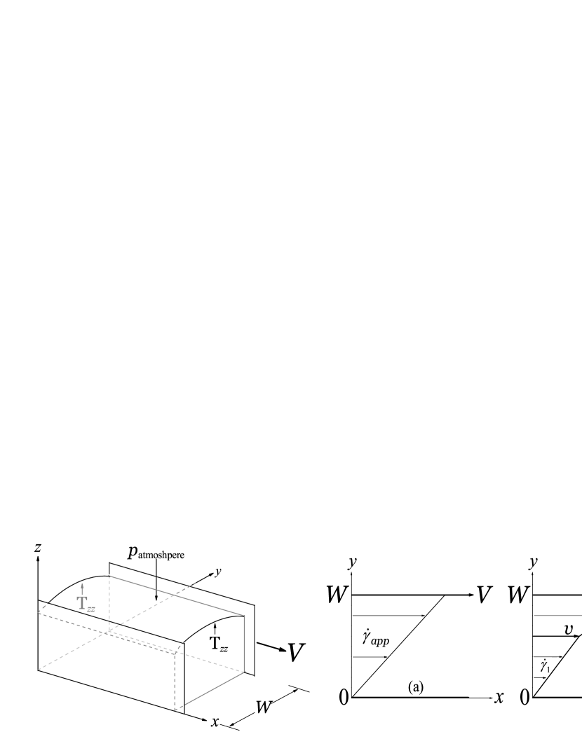
Figure 2: (Left) Schematic diagram of planar Couette flow. The plate in the $y=0$ plane is stationary whilst a parallel plate a distance $W$ away moves with velocity $V$. The free surface at large $z$ is open to the atmosphere. (Right) Velocity profiles for an applied average shear rate $\dot{\gamma}_{\textrm{app}}=\frac{V}{W}$: (a) unbanded or (b) shear banded. For banded flow $\dot{\gamma}_{1}=\frac{v}{w_{1}}$ and $\dot{\gamma}_{2}=\frac{V-v}{w_{2}}$, where $w_{1}$ and $w_{2}$ are the widths of the two shear bands.

Figure 3: (a) Flow curve (thick line) and constitutive curve (thin line) for shear banding flows. Banding occurs on the stress plateau at ${\rm T}^{\ast}_{xy}$, for applied shear rates $\dot{\gamma}_{\textrm{app}}$ such that $\dot{\gamma}_{1}\leq\dot{\gamma}_{\textrm{app}}\leq\dot{\gamma}_{2}$. A ‘lever’ rule relates the widths of the shear bands to the applied shear rate, $w_{1}=W(\dot{\gamma}_{2}-\dot{\gamma}_{\textrm{app}})/(\dot{\gamma}_{2}-\dot{\gamma}_{1})$ and $w_{2}=W-w_{1}$. (b) Profile of the fluid surface (meniscus) between flat plates (flow in the $\hat{x}$ direction). Each band has a circular profile, and the surface is continuous and differentiable; $\phi_{1}$ and $\phi_{2}$ are the contact angles at the two plates. The contact lines between fluid and plates move up and down as the widths of the shear bands alter; $H$ is the height difference between the contact lines. Note that the curvatures may be positive or negative.

Stress balance (Eq. 3) implies that $\text{T}_{xy}$ and $\text{T}_{yy}$ are the same in each shear band. This implies that $\Sigma_{xy}^{(1)}=\Sigma_{xy}^{(2)}$, where ⁽¹⁾ and ⁽²⁾ refer to the two shear bands. Moreover,

$$\Sigma_{yy}^{(1)}-p_{1}=\Sigma_{yy}^{(2)}-p_{2}.$$ (4)

Since the normal stresses will generally be different in the two bands, the pressures $p_{1}$ and $p_{2}$ will differ. These pressures must then balance, together with $\Sigma_{zz}$, against the curvature of the meniscus and the atmospheric pressure $p_{atm}$:

$$\text{T}_{zz}^{(i)}=-p_{i}+{\Sigma}_{zz}^{(i)}(\gamma_{i}) =-p_{atm}-\frac{\gamma_{s}}{R_{i}}\quad(i=1,2),$$ (5)

where $R_{i}$ is the radius of curvature of the meniscus in the $i$th band and $\gamma_{s}$ is the surface tension. From Eq. (4) the difference in $\text{T}_{zz}$ between the two bands is given by the difference in the second normal stress differences, $\text{T}_{zz}^{(1)}-\text{T}_{zz}^{(2)}=N_{2}^{(2)}-N_{2}^{(1)}$. Making use of this and Eq. (5), we can relate the second normal stress differences to the radii of curvature of the two bands

$$\frac{\Delta N_{2}}{\gamma_{s}}=\frac{1}{R_{2}}-\frac{1}{R_{1}},$$ (6)

where $\Delta N_{2}=N_{2}^{(2)}-N_{2}^{(1)}$. This can be easily calculated for a given constitutive relation, and together with the surface tension defines a characteristic ‘elasto-capillary’ length for the shear banding configuration:

$$\zeta=\frac{\gamma_{s}}{|\Delta N_{2}|}.$$ (7)

The three equations (4, 5) relate four unknown quantities: the pressures and meniscus curvatures in each band. By eliminating the pressures we can relate curvature radii, but more information is needed to absolutely determine the shape. This will follow by constructing a continuous and smooth meniscus. The balance at the meniscus, Eq. (5), determines the pressure in each band in terms of the meniscus curvature. We will find below that the curvatures must change in order to maintain a physical meniscus, which thus determines the pressure in each band.

III Meniscus Shape and Integrity

III.1 General Shape (two bands)

We ignore deviations due to complex flows near the contact line, and approximate the meniscus of each band as the arc of a circle of radius $R_{i}$, which may be positive or negative. We demand continuity of the surface and its tangent at the interface between two bands. The conditions above can be fulfilled either by:

1. the contact angles being fixed and the fluid adopting a height $H$ difference between the contact lines along each plate (movement of the contact lines has been observed by Crawley and Graessley (1977)); this height difference will vary in response to the widths of the shear bands;

2. the contact lines being pinned such that $H$ is fixed and the contact angles vary in response.

In both cases the meniscus profiles are governed by the same equations. The height profiles of the two bands are given by

$$h(y)=\begin{cases}R_{1}\left(\sqrt{1-\left(\dfrac{y}{R_{1}}+\cos\phi_{1}\right)^{2}}-\sin\phi_{1}\right)&\quad(0\leq y\leq w_{1})\\[12.91663pt] R_{2}\left(\sqrt{1-\left(\dfrac{y-W}{R_{2}}-\cos\phi_{2}\right)^{2}}-\sin\phi_{2}\right)+H&\quad(w_{1}<y\leq W)\>,\end{cases}$$ (8)

where $\phi_{1}$ and $\phi_{2}$ are the contact angles at either wall, and $h(0)=0$ and $h(W)=H$. Continuity of $h$ at $y=w_{1}$ requires

$$H=(R_{1}-R_{2})\sqrt{1-\Big{(}\frac{w_{1}}{R_{1}}+\cos\phi_{1}\Big{)}^{2}}+R_{2}\sin\phi_{2}-R_{1}\sin\phi_{1}\;,$$ (9)

and continuity of $h^{\prime}$ at $y=w_{1}$ requires

$$\frac{w_{1}}{R_{1}}+\frac{w_{2}}{R_{2}}=-\cos\phi_{1}-\cos\phi_{2}\;.$$ (10)

III.2 Fixed Contact Angles

We allow the surface tensions at the fluid, walls, and atmosphere interface to determine the contact angles and assume that the contact angles persist through the onset of banding. Then Eq. (6) and Eq. (10) completely specify the shape:

$$\hat{R}_{1}=\frac{1}{-\cos\phi_{1}-\cos\phi_{2}-\hat{w}_{2}A}\quad\text{and}\quad\hat{R}_{2}=\frac{1}{-\cos\phi_{1}-\cos\phi_{2}+\hat{w}_{1}A}\;,$$ (11)

where the dimensionless distortion parameter

$$A\equiv\frac{W\Delta N_{2}}{\gamma_{s}}=-\frac{W}{\zeta}$$ (12)

controls the shape. In the limit of high surface tension, $|A|\simeq 0$, both radii are equal and completely determined by the contact angles. We have chosen negative values for $A$ here since we expect $N_{2}^{(2)}<N_{2}^{(1)}\leq 0$ in the high shear rate band for most polymer and micellar solutions (a similar analysis can be done for $A>0$). In Section IV we analyze recent experiments and estimate $-A\sim 0.8$ - $3$ for shear banding wormlike micelles and $-A\sim 3$ - $140$ for entangled polymer solutions.

III.3 Integrity of Meniscus

An interface solution exists under two conditions, one mathematical and the other practical:

• The curves should not have infinite slope or pass through each other. This leads to the condition

  $$\Big{|}\hat{w}_{2}\cos\phi_{1}-\hat{w}_{1}\cos\phi_{2}-\hat{w}_{1}\hat{w}_{2}A\Big{|}<1\>.$$ (13)

• The increase $H$ in height across the gap should not be large enough for the sample to climb out of the cell. This obviously depends on the loading conditions, and can generally preempt the mathematical condition above.

III.4 Equal Contact Angles

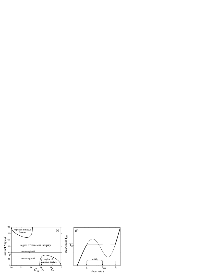
Figure 4: (a) Integrity contours for equal contact angles $\phi_{2}=\phi_{1}=\phi$, for $A=-3.5$. For a wall and fluid combination that fixes $\phi=60^{\circ}$ all shear band widths are allowed and the applied shear rate will traverse the plateau. For a wall and fluid combination that fixes $\phi=40^{\circ}$ not all shear rates accessible; the surface of the fluid becomes fracture for some widths $\hat{w}_{2}$ of the high shear rate band satisfying $\hat{w}^{-}_{2}<\hat{w}_{2}<\hat{w}^{+}_{2}$. All widths allow meniscus integrity for $|\cos\phi|<\cos\phi^{\ast}=0.661$. (b) Flow curve (thick line) for a wall and fluid combination with $\phi=40^{\circ}$, showing the inaccessible segment of the stress plateau.

We first consider equal contact angles $\phi_{1}=\phi_{2}=\phi$, for which the meniscus integrity condition is

$$\left|(\hat{w}_{2}-\hat{w}_{1})\cos\phi-\hat{w}_{1}\hat{w}_{2}A\right|<1,$$ (14)

where the criterion

$$-1-\cos\phi<\frac{\hat{w}_{i}}{\hat{R}_{i}}<1-\cos\phi$$ (15)

is required for Eq. (9) to yield real solutions. Fig. 4a shows regions of integrity for $A=-3.5$ and two chosen cases. For a wall and fluid combination that fixes $\phi=60^{\circ}$ the entire shear stress plateau is accessible and supports a integral meniscus. However, for a wall and fluid combination that fixes $\phi=40^{\circ}$ some values of $w_{2}$ are not allowed and the corresponding applied shear rates are not accessible on the stress plateau. For small contact angles the low shear rate portion of the plateau is accessible, while for high contact angles the high shear rate portion of the plateau is accessible. Fig. 4b shows a possible flow curve for the $\phi=40^{\circ}$ case.

To understand the lack of integrity of the meniscus we must examine the meniscus shapes. These are shown in Fig. 5 as a function of increasing the applied shear rate $\dot{\gamma}_{\textrm{app}}$ across the stress plateau, for both a integral case ($\phi=60^{\circ}$) and an non-integral case ($\phi=40^{\circ}$), for $A=-3.5$. Note that banding first initiates when the high shear rate band develops a non-zero width, i.e. when $\hat{w}_{2}$ grows from zero for $\dot{\gamma}_{\textrm{app}}\geq\dot{\gamma}_{1}$.

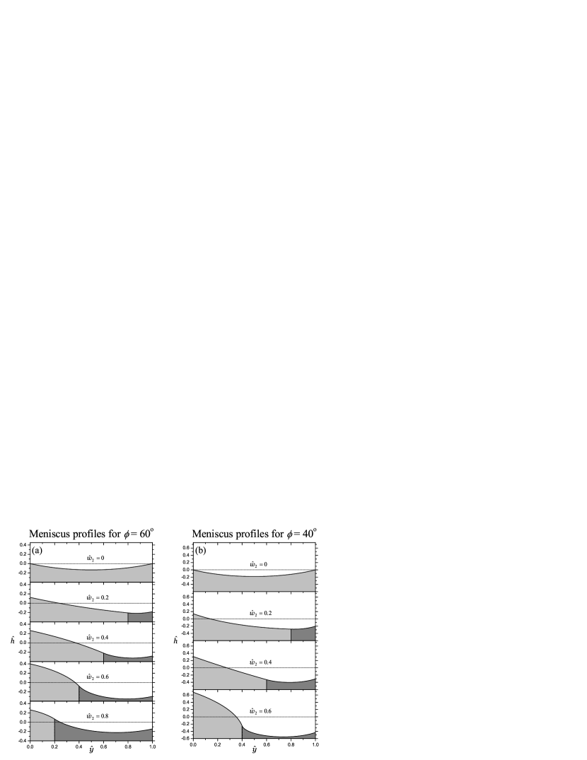
Figure 5: (a,c) Meniscus profiles $h(y)$; and (b,d) height difference $\hat{H}$ and curvatures normalized by the gap size, $\frac{w_{i}}{R_{i}}$, as a function of the high shear band width $\hat{w}_{2}$; for $A=-3.5$. The dotted lines are the integrity limits on $\frac{w_{i}}{R_{i}}$ from Eq. (15). For the $\phi=60^{\circ}$ case (a,c) the surface remains integral for all shear rates in the plateau region, while for the $\phi=40^{\circ}$ case (bd) the surface of the fluid will fracture on some portion of the stress plateau.

Consider first the $\phi=60^{\circ}$ case (Fig. 5a). At $\hat{w}_{2}=0.2$ the contact line of the higher rate shear band has dropped while that of the lower shear rate band has risen. Both surfaces have negative radii of curvature. By $\hat{w}_{2}=0.4$ the radius of curvature of the lower shear rate band has become positive. The height difference between the contact lines increases and reaches a maximum at $\hat{w}_{2}\simeq 0.65$, but the surface still maintains its integrity. For larger $\hat{w}_{2}$ the height difference decreases until shear banding ceases at $\hat{w}_{2}=1$ ($\dot{\gamma}_{\textrm{app}}=\dot{\gamma}_{2}$). For the $\phi=40^{\circ}$ case, however (Fig. 5b), the integrity of the surface cannot be fulfilled when the width of the high shear rate band satisfies $0.6<\hat{w}_{2}<0.83$ (see Fig. 5d).As can be see in Fig. 5b, the interface develops a kink immediately before the onset of fracture. In the region of fracture we find that there is no continuous solution to the meniscus profiles.

Figures 5(cd) show the height difference $\hat{H}$, and the surface curvatures for the different shear bands $\frac{w_{i}}{R_{i}}$ normalized by the respective band size, as a function of shear band width $\hat{w}_{2}$ (or equivalently the applied shear rate $\dot{\gamma}_{\textrm{app}}$). The surface will maintain integrity so long as solutions for $h^{\prime}(y)$ (and consequently $H$) exist. The dotted lines indicate between which values $\frac{\hat{w}_{1}}{\hat{R}_{1}}$ and $\frac{\hat{w}_{2}}{\hat{R}_{2}}$ must lie in order to maintain integrity.

The integrity contours for a range of distortion parameters $A$ are shown in Fig. 6, and the different regions of integrity are summarized in Table 1. For $A>-2$ the meniscus is always integral. For $-4<A<-2$ the meniscus is integral for contact angles satisfying

$$\cos^{2}\phi\leq\cos^{2}\phi^{\ast}=|A|\left(1-\frac{|A|}{4}\right).$$ (16)

For large magnitude $|A|>4$ the meniscus looses integrity at all contact angles, for some regions of the stress plateau. For $A<0$, as in our case, this occurs when the width of the high low shear rate band is between the limits

$$\hat{w}_{2}^{\pm}=\frac{1}{2}\left(1+\frac{2\cos\phi}{|A|}\right)\left[1\pm\sqrt{1-\frac{4|A|\left(1+\cos\phi\right)}{\left(|A|+2\cos\phi\right)^{2}}}\right].$$ (17)

These limits also apply for $-4<A<-2$, for $|\cos\phi|\geq|\cos\phi^{\ast}|$.

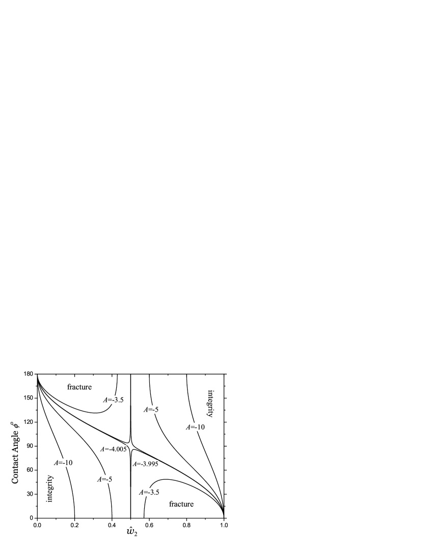
Figure 6: Regions of integrity for equal contact angles $\phi$ and for different values of the distortion parameter $A$.

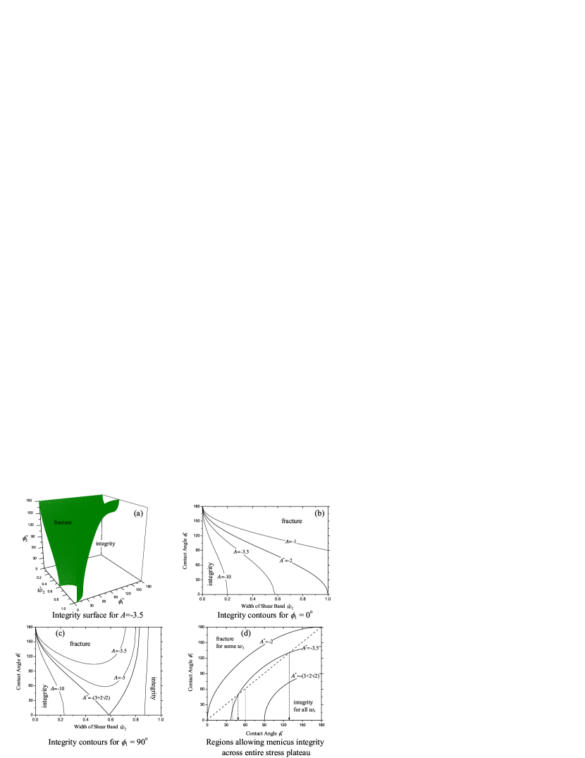
Figure 7: (ab) Regions of integrity as a function of contact angles $\phi_{1}$ and $\phi_{2}$, and the width $\hat{w}_{2}$ of the high shear rate band for distortion parameter $A=-3.5$. The meniscus is integral for any combination of $\hat{w}_{2}$, $\phi_{1}$, and $\phi_{2}$ in the integral region. Fig. 4a is the intersection of this integrity surface with the plane $\phi_{1}=\phi_{2}$. For $A=-1$ and $\phi_{2}<90^{\circ}$ the meniscus is integral for all $\hat{w}_{2}$ (i.e. across the entire stress plateau). For $A<A^{*}=-2$ the meniscus fractures at some shear band width $\hat{w}_{2}$ for all contact angles $\phi_{2}$. (c) Integrity contours for $\phi_{2}=90^{\circ}$. The meniscus fractures at some $\hat{w}_{2}$ for all $\phi_{2}$ if $A<-(3+2\sqrt{2})$. (d) Contours specified by $A^{\ast}$ as a function of contact angles $(\phi_{1},\phi_{2})$ that enclose regions of integrity across the whole shear stress plateau. On the dashed line $\phi_{1}=\phi_{2}$. For $A^{*}=-3.5$ the dotted arrows indicates the contact angles for which the meniscus will be integral for all $\hat{w}_{2}$. The dotted lines indicate fracture at some $\hat{w}_{2}$ as shown in Fig. 4a.

Range of $A$			Integrity of meniscus
	$A$	$<-4$	Fractures for all contact angles $\phi$, for $\hat{w}^{-}_{2}<\hat{w}_{2}<\hat{w}^{+}_{2}$.
$-4<$	$A$	$<-2$	Fractures for $|\cos\phi|>|\cos\phi^{\ast}|$ and $\hat{w}^{-}_{2}<\hat{w}_{2}<\hat{w}^{+}_{2}$.
$-2<$	$A$	$<\;\;\>0$	Integral for all contact angles $\phi$.

Table 1: Criteria for (lack of) integrity as a function of the distortion parameter $A$, for equal contact angles $\phi_{1}=\phi_{2}=\phi$.

III.5 Different Contact angles

For different contact angles the situation is more complex. For $A<0$ the meniscus remains integral for all $\hat{w}_{2}$ for $A>-8$ and

$$\cos\phi_{2}>\left[\sqrt{|\cos\phi_{1}-1|}-\sqrt{|A|}\right]^{2}-1.$$

For $A<-8$ the meniscus fractures somewhere along the stress plateau for any combination of contact angles. This condition is illustrated in Fig. 7, which shows the regions of integrity and fracture as a function of both contact angles, for $A=-3.5$ (Fig. 4a is a slice through this figure for $\phi_{1}=\phi_{2}$). Fig. 7b shows that an asymmetry in contact angle increases the region for meniscus fracture. For $\phi_{1}=0$, corresponding to a wetting surface, a larger contact angle leads to a fractured meniscus for $|A|<2$, which would always be integral for equal contact angles.

III.6 Pinned Contact Lines

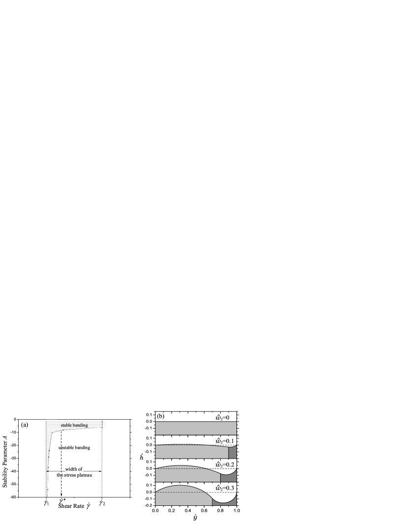
Figure 8: Stability regions of profiles for contact lines pinned such that $H=0$. (a) The full width of the shear stress plateau is accessible for $-8<A<0$. For $A<-8$ the surface will fracture at some applied shear rate $<\dot{\gamma}^{\ast}$. (b) Meniscus profiles for $A=-8$. The surface maintains integrity for applied shear rates up to $\dot{\gamma}^{\ast}$ at which rate the high shear rate band has achieved $w_{2}=0.3$ of the width of the gap.

For pinned contact lines we ascribe a particular value to $H$. Eqs (6), (9) and  (10) are not sufficient to specify $R_{1},\;R_{2},\;\phi_{1}$ and $\phi_{2}$; the fourth condition is the requirement of volume conservation for an incompressible fluid. Fig. 8 is a typical example in which the contact lines have been pinned so that their difference in height $H$ is zero. For applied shear rates associated with the stress plateau the meniscus contorts but retains integrity for all shear rates when $-8<A<0$; for $A<-8$ not all shear rates are accessible and the meniscus will fracture at some shear rate.

III.7 Three Bands

Fig. 1 shows an example of three shear bands, visualized in a cone-and-plate rheometer by Britton and Callaghan (1997) using NMR velocimetry. Three bands have not been observed in cylindrical Couette flow, and this difference was rationalized by Adams, Fielding, and Olmsted (2008) as due to a combination of boundary conditions that favor the low shear rate phase and the relatively weak stress gradient of cone-and-plate flow. Motivated by this result, we have calculated the distortion of the meniscus in such a configuration and find that a three band state does indeed allow meniscus integrity, for certain ranges of parameters. This analysis is given in Appendix C.

IV Comparison with the literature

IV.1 Theoretical Method

We examine existing data in the literature, which exhibits both stable shear banding across the entire stress plateau and an instability such that the entire stress plateau could not be accessed; we then assess whether or not meniscus fracture is expected, based on an estimation of the distortion parameter $A=W\Delta N_{2}/\gamma_{s}$. We fit the data from the flow curves, including the stress plateau and the shear rates $\dot{\gamma}_{1}$ and $\dot{\gamma}_{2}$ in the two shear bands, to both the Giesekus and Johnson-Segalman (JS) constitutive models. From the models we can evaluate the predicted second normal stress difference $N_{2}$ in the two shear bands (see Appendix B), while the gap size $W$ is taken from the experimental conditions and the surface tension $\gamma_{s}$ is estimated using literature values. With this in hand we can then compare the stability or instability of banding states, inferred from the experiments, with our calculations. Since the contact angles are unknown, we can only determine whether our criteria for instability are consistent with the numerical values for $A$ (assuming equal contact angles). We are also limited by the quality of the available constitutive models: neither the JS or Giesekus models are expected specifically apply to wormlike micelles, but they can support shear banding and have non-zero second normal stresses. These models, developed for polymer melts, may be more applicable to semi-dilute polymeric solutions, which have an explicit Newtonian solvent. Fischer and Rehage (1997), Yesilata, Clasen, and McKinley (2006), and Helgeson et al. (2009) show that the steady state non-linear rheology and shear thinning of worm-like micelles is well described by the Giesekus model; we offer the Johnson-Segalman model for comparison. In fact, the two models yield very similar quantitative predictions and thus do not substantially differ insofar as determining the properties of the meniscus.

IV.2 Wormlike Micellar Solutions

Wormlike micellar solutions of both cetyltrimethylammonium (CTAB) and cetylpyridinium choloride/sodium salicilate (CPCl/NaSal) have been extensively studied. Fig. 9 shows the data of a CTAB solution, as measured by Helgeson et al. (2009) and fit by them to the diffuse Giesekus model. In this case the entire stress plateau was accessible. We have also fitted it to the non-diffuse Giesekus and JS models. Strictly, one should fit the stress plateau using a non-local (or diffuse) model (Lu, Olmsted, and Ball, 2000); however, our fits obtained by choosing the stress plateau ‘by hand’ differ insignificantly from more precise fitting. Hence we use a local model for the remaining fits in this paper. The Giesekus model fits the high shear rate branch much better than does the JS model.

The fitting parameters are shown in Table 2. The difference between the diffuse and non-diffuse Giesekus models values for $\Delta N_{2}$ is less than 3%. We estimate the distortion parameter to be $A\simeq-0.8$, which is well within range ($A\geq-2$, from Table 1) for which we expect to find stable shear bands across the entire stress plateau for all contact angles.

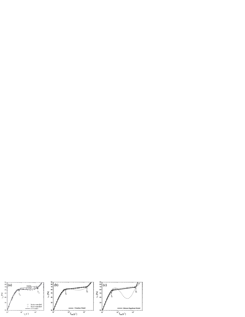
Figure 9: (a) Flow curve for a CTAB solution fitted to the (numerical) diffuse Giesekus model, measured in a Couette rheometer with a gap $W=0.5\,\textrm{mm}$ (Helgeson et al., 2009). Fits to the non-diffuse Giesekus (b) and JS (c) models (fitting parameters are given in Table 2).

					Parameters
Figure	Material	$\eta_{o}/(\textrm{Pa\,s})$	$\text{T}/^{\circ}\text{C}$	$W/\textrm{mm}$	$G/\textrm{Pa}$	$\tau/\textrm{s}$	$a$	$\epsilon$	$\dot{\gamma}_{1}/\textrm{s}^{-1}$	$\dot{\gamma}_{2}/\text{s}^{-1}$	$\frac{\Delta N_{2}}{G}$	$A$
Fig. 9	CTAB	2.1	32	0.5	112	0.018	0.9	0.008	65	1530	-0.48	-0.8	Gi
					115	0.017	0.43	0.022	40	1430	-0.52	-0.8	JS
Fig. 10	CPCl	18	30	0.5	165	0.11	0.88	0.015	11	60	-0.38	-0.9	Gi
	8%				168	0.09	0.41	0.056	8	90	-0.48	-1.2	JS
Fig. 11	CPCl	240	20	0.5	260	0.94	0.87	0.002	1	54*	-0.60	-2.2	Gi
	12%				268	0.88	0.38	0.010	0.85	54*	-0.49	-1.9	JS

Table 2: Parameters used to fit the flow curves in Figs. 9, 10, and 11, for the Giesekus (Gi) or Johnson-Segalman (JS) models. We estimate a surface tension $\gamma_{s}\simeq 37\,\text{mN/m}$ for aqueous CTAB (Christian et al., 1998) and $\gamma_{s}\simeq 32\>\text{mN/m}$ for CPCl/NaSal (Akers and Belmonte, 2006). For the stable solutions (CTAB and 8% CPCl) the shear rate $\dot{\gamma}_{2}$ of the high shear rate band was taken from the end of the stress plateau, while for the unstable solution (12% CPCl) $\dot{\gamma}_{2}$ was estimated from the scaling in Fig. 8 of Berret, Porte, and Decruppe (1997).

We have found a few experiments that show a clear instability as the stress plateau is traversed, or that cannot reach the end of the stress plateau. Berret and co-workers (Berret, Roux, and Porte (1994) and Berret, Porte, and Decruppe (1997)) studied CPCl/NaSal solutions at different concentrations and temperatures, in a cone-and-plate rheometer with a free surface. They found stable stress plateaus at micellar solutions close to a non-equilibrium critical point, where the difference between the shear banding phases vanishes. Farther from the critical point, where the shear banding phases are more distinct, and hence one expects $\Delta N_{2}$ to be larger, they report unstable stress plateaus (see Fig. 6 of Berret, Porte, and Decruppe (1997)). Fig. 10 show the data and fits for an $8\%$ solution at $T=30^{\circ}\,\textrm{C}$, which was close to the non-equilibrium critical point. The fitting leads to a distortion parameter between $A\simeq-1.0$ and $A\simeq-1.3$, which is consistent with the meniscus maintaining integrity across the entire stress plateau.

The data for an unstable CPCl solution are shown in Fig. 11, at $12\%$ and $T=20^{\circ}\,\textrm{C}$. In this case the stress plateau can only be traversed as far as $\dot{\gamma}_{\textrm{app}}=7.1\,\textrm{s}^{-1}$, at which point the fluid became unstable (Berret, Porte, and Decruppe, 1997). To calculate the distortion parameter we require the shear rate $\dot{\gamma}_{2}$ in the high shear rate phase, which we estimate from Fig. 8 of (Berret, Porte, and Decruppe, 1997) to be $\dot{\gamma}_{2}\simeq 54\,\textrm{s}^{-1}$. This is consistent with the measurements of the high shear rate branch performed by Lopez-Gonzalez, Holmes, and Callaghan (2006) on the same material with a free surface: Fig. 11 of their paper shows a a $10\%$ sample at $25^{\circ}\,\textrm{C}$. Fits to the Giesekus and JS models respectively yield $A\simeq-2.4$ and $A\simeq-2.0$, for the $12\%$ sample of Berret, Porte, and Decruppe (1997), at $T=20^{\circ}\,\textrm{C}$. In the range $A<-2$ we expect meniscus fracture for some contact angles, and across some region of the stress plateau. The experiments show an instability at $\hat{w}_{2}=0.12$. Fig. 6 shows that such a small value of $\hat{w}_{2}=0.12$ and $A\lesssim-2$ would be consistent with a contact angle near $180^{\circ}$, or complete wetting. We caution, however, against using the numerical results from applying these fairly crude constitutive models. It is clear, however, that the distortion parameter predicts that the 12$\%$ fluid at $T=20^{\circ}\,\textrm{C}$ should be more unstable than the $8\%$ fluid at $T=30^{\circ}\,\textrm{C}$. We have also estimated the distortion parameter from the closely related experiments of Lopez-Gonzalez, Holmes, and Callaghan (2006) (see Fig. 5 from that paper), for which we estimate $-A\simeq 2.3-2.6$, again just into the predicted range of possible meniscus fracture.

Figure 10: Data and fitted constitutive curves for the experiments of Berret, Porte, and Decruppe (1997) on CPCl at $8\%$ (by weight) and $T=30^{\circ}\,\textrm{C}$, using the (a) Giesekus (b) JS models. The geometry was a cone and plate rheometer. Parameters are shown in Table 2.

Figure 11: Data and fitted constitutive curves for the experiments of Berret, Porte, and Decruppe (1997) on CPCl at $12\%$ (by weight) and $T=20^{\circ}\,\textrm{C}$, using the (a) Giesekus (b) JS models. The geometry was a cone and plate rheometer. Parameters are shown in Table 2. The fluid became unstable at the rightmost data point $\blacksquare$, at $\dot{\gamma}_{\textrm{app}}=7.2\,\textrm{s}^{-1}$. The open circle $\circ$ shows our estimate of the shear rate in the high shear rate branch based on extrapolation from the rheology of Fig. 8 of Berret, Porte, and Decruppe (1997), together with the temperature dependences in Figs. 5 and 7 of the same reference and Fig. 4 of Berret, Roux, and Porte (1994) .

We have collected much of the available data in the literature in Table 3. In many cases the full banding profile was found (noted as ‘stable’ in Table 3), and in all of these cases we calculated $A$ to be in the range $A>-2$, the meniscus retains integrity (Table 1). Similarly, all of the unstable data that we have found corresponds to $A<-2$, for which meniscus fracture is expected for some contact angles (Table 1).

			Model Parameters											Instability at
Material	Cell	$\text{T}/^{\circ}\text{C}$	$W/\textrm{mm}$	$G/\textrm{Pa}$	$\tau/\textrm{s}$	$a$	$\epsilon$	$\dot{\gamma}_{1}/\textrm{s}^{-1}$	$\dot{\gamma}_{2}/\text{s}^{-1}$	$\frac{\Delta N_{2}}{G}$	$A$			$\dot{\gamma}_{\textrm{app}}^{\ast}/\textrm{s}^{-1}$	$\hat{w}_{2}^{\ast}$
CTAB	C	32	0.17	69	0.11	0.92	0.005	6	330	-0.71	-0.2	Gi	stable
				70	0.11	0.5	0.01	5.5	450	-0.53	-0.2	JS	stable
CPCl	CP	20	0.5	94	0.62	0.92	0.02	1.5	11	-0.48	-0.7	Gi	stable
6%				96	0.55	0.38	0.055	1.2	13	-0.51	-0.8	JS	stable
CTAB	C	32	0.5	112	0.018	0.9	0.008	65	1530	-0.48	-0.7	Gi	stable
Fig. 9				115	0.017	0.43	0.022	40	1430	-0.52	-0.8	JS	stable
CPCl	CP	30	0.5	165	0.11	0.88	0.015	11	60	-0.38	-1.0	Gi	stable
8% Fig. 10				168	0.09	0.41	0.056	8	90	-0.48	-1.3	JS	stable
CTAB	C	32	1	69	0.11	0.92	0.005	6	330	-0.71	-1.3	Gi	stable
				70	0.11	0.5	0.01	5.5	450	-0.53	-1.0	JS	stable
CPCl	C	21.5	1	108	0.48	0.88	0.012	2.5	26	-0.44	-1.5	Gi	stable
6%				105	0.51	0.65	0.036	1.5	27	-0.45	-1.5	JS	stable
CPCl	CP	30	0.5	291	0.15	0.84	0.002	8	*187	-0.50	-2.3	Gi	unstable	80	0.40
12%				282	0.14	0.57	0.021	6.5	*187	-0.42	-1.8	JS	unstable		0.41
CPCl	CP	20	0.5	260	0.94	0.87	0.002	1	*54	-0.59	-2.4	Gi	unstable	7.1	0.12
12% Fig. 11				268	0.88	0.38	0.010	0.85	*54	-0.49	-2.0	JS	unstable		0.12
CPCl	CP	25	0.6	224	0.32	0.92	0.007	2.5	*70	-0.62	-2.6	Gi	unstable	43	0.60
10%				225	0.29	0.4	0.022	2.2	*70	-0.54	-2.3	JS	unstable		0.60
CTAB	C	28	1.13	267	0.21	0.89	0.016	4	90	-0.59	-4.8	Gi	*unstable	(40)	(0.42)
				290	0.18	0.43	0.033	3	95	-0.56	-5.0	JS	*unstable		0.40

Table 3: Values of the distortion parameter $A$ calculated from experimental studies on worm like micellar solutions using either the Giesekus (Gi) or JS models. “Stable” experiments accessed the full stress plateau, while in “unstable” cases an instability occurred at the apparent shear rate $\dot{\gamma}_{\textrm{a}pp}^{\ast}$ for a high shear rate band of width $\hat{w}_{2}^{\ast}$. The first column identifies the figure above that demonstrates the fit, and the weight fraction used for the experiments of Berret, Porte, and Decruppe (1997). We estimate a surface tension $\gamma_{s}\simeq 37\,\text{mN/m}$ for aqueous CTAB (Christian et al., 1998) and $\gamma_{s}\simeq 32\>\text{mN/m}$ for CPCl/NaSal (Akers and Belmonte, 2006).

IV.3 Polymer Solutions

Wang and co-workers revived the experimental study of entangled polymers with new experiments that clearly show shear banding (Tapadia and Wang, 2003; Hu et al., 2007; Boukany and Wang, 2007, 2009). Tapadia and Wang’s first experiments, on polybutadiene (PBD) entangled in its own oligomer, suggested shear banding by what they referred to as an ‘entanglement disentanglement transition’ (EDT); this data is also broadly consistent with theories based on the Doi-Edwards tube model (Adams and Olmsted, 2009b, a; Wang, 2009). In the earliest experiments they apparently used a free surface, and commented that some small edge fracture or instability could have occurred, but that its effects were negligible.

While attempting to reproduce these experiments, Inn, Wissbrun, and Denn (2005) found significant edge fracture and instability in the region of the transition and the stress plateau, and concluded that the surface instability and associated mass loss was responsible for the effects. This was then studied by Sui and McKenna (2007) using cone-and-plate rheometers with gap sizes at the rim of $W=0.267\,\textrm{mm}$ and $W=1.363\,\textrm{mm}$. They found significant edge fracture or instability accompanying the shear banding transition, but their results suggested that the surface instability could be a consequence, rather than a cause, of the shear banding transition (or EDT). This is seen most clearly in Fig. 5 of Sui and McKenna (2007), which shows that the stress plateau can be traversed when a plastic film is used to suppress the instability at the surface (Philips and Wang performed the film-suppressed experiments). Schweizer (2007) also found that surface deformation accompanied the banding, or EDT, in similar materials. More recently, Ravindranath and Wang (2008) and Li and Wang (2010) have verified that the shear banding (or EDT) transition can persist when even when surface effects are suppressed.

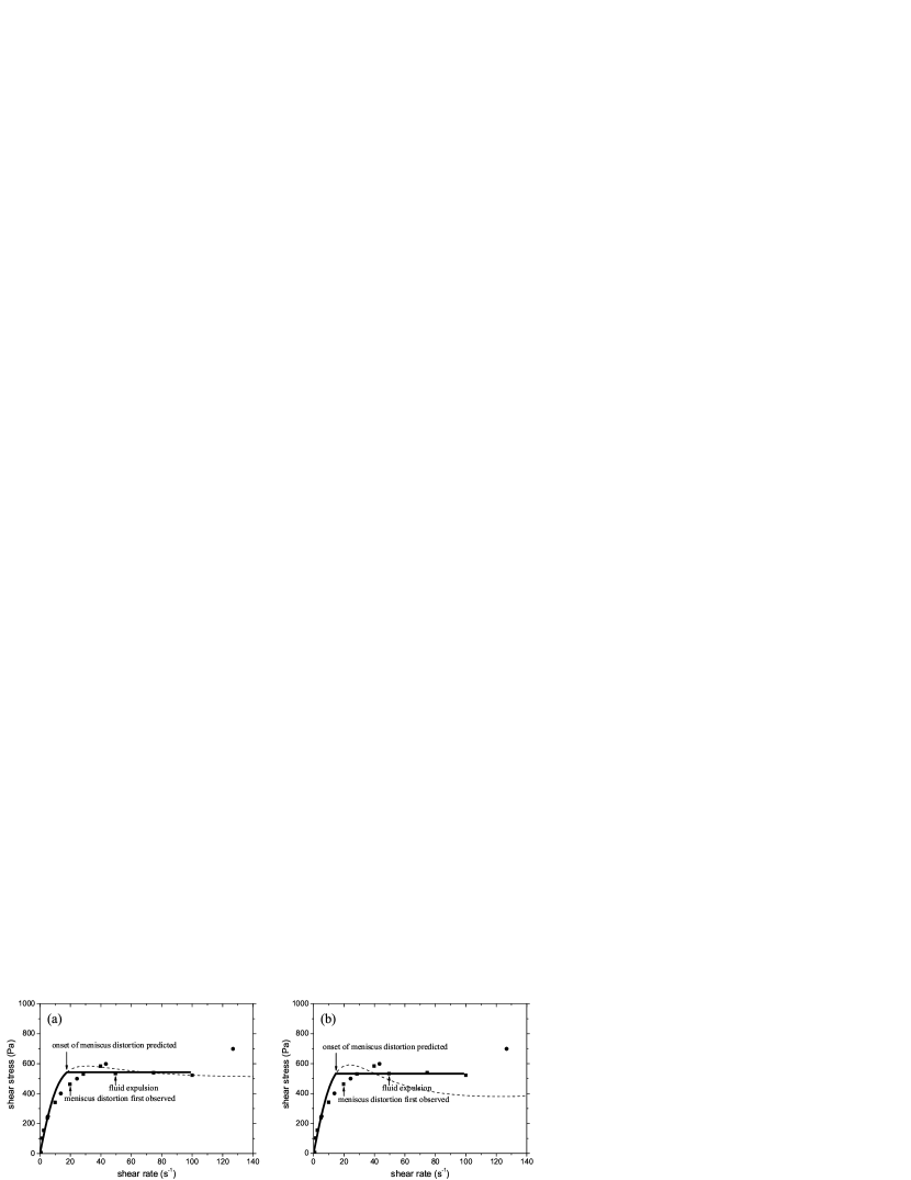
Figure 12: Data and flow curves for the experiments of Sui and McKenna (2007) on SRM 2400, using a $6^{\circ}$ cone angle. $\blacksquare$ indicates rate-controlled and • stress-controlled rheometry. Fits are to the (a) Giesekus and (b) Johnson Segalman models.

Figure 13: Data and flow curves for the experiments of Sui and McKenna (2007) on PBD under controlled strain rate conditions, fitted to either the Giesekus (a) or JS (b) models. The Giesekus fits show several different fits, to illustrate the difficulty of precise characterization of the constitutive models. Table 4 shows that the distortion parameter $A$ is only very weakly sensitive to these different fits. Here, $\blacktriangle$ indicates $1^{\circ}$ gap and • indicates $6^{\circ}$.

		cone			Parameters									Instability at
Material	$\eta_{o}/(\textrm{Pa\,s})$	angle	$\text{T}/^{\circ}\text{C}$	$W/\textrm{mm}$	$G/\text{Pa}$	$\tau/\text{s}$	$a$	$\epsilon$	$\dot{\gamma}_{1}/\text{s}^{-1}$	$\dot{\gamma}_{2}/\text{s}^{-1}$	$\frac{\Delta N_{2}}{G}$	$A$		$\dot{\gamma}_{\textrm{app}}/\textrm{s}^{-1}$	$\hat{w}_{2}$
SRM 2490	$85$	1∘	room	0.267	1060	0.047	0.93	0.01	18	300*	-0.571	-6.2	Gi	none ​​​
			($\sim 24$)	0.267	1040	0.048	0.36	0.03	17	300*	-0.461	-4.9	JS	noted
		6∘		1.363	1060	0.047	0.93	0.01	18	300*	-0.571	-32	Gi	50	0.11
				1.363	1040	0.048	0.36	0.03	17	300*	-0.461	-25	JS		0.12
PBD	$3.9\times 10^{4}$	1∘	30	0.267	5150	7.2	0.87	0.0001	0.1	50	-0.717	-33	Gi	2.5	0.05
					”	”	0.90	”	”	71	-0.709	-32	Gi	”	”
					”	”	0.93	”	”	103	-0.697	-32	Gi	”	”
					5170	7.1	0.68	0.001	0.08	60	-0.515	-24	JS	”	”
		6∘		1.363	5150	7.2	0.87	0.0001	0.1	50	-0.717	-167	Gi	0.25	0.00
					”	”	0.90	”	”	71	-0.709	-166	Gi	”	”
					”	”	0.93	”	”	103	-0.697	-163	Gi	”	”
				1.363	5170	7.1	0.68	0.001	0.08	50	-0.515	-121	JS	”	”

Table 4: Parameters used to fit the flow curves in Figure 12a and 12b to the Johnson-Segalman (JS) and Giesekus (Gi) and evaluate the distortion parameter $A$ for the study of Sui and McKenna (2007) of polybutadiene-in-oligomer (PBD) and polyisobutylene-in-pristane (SRM 2490) solutions. The surface tension of pristane is around $26\,\text{mN/m}$ (Bascom, Cottington, and Singleterry, 1964) and that of 1,4 PBD is around $30\,\text{mN/m}$ (Brandrup and Immergut, 1989). The PBD was fit to the Giesekus model for several possibilities to illustrate the robustness of the parameter $A$. ^∗For the SRM solutions the shear rate $\dot{\gamma}_{2}$ of the high shear rate band was estimated based on the parametrization of the shear thinning behaviour of the low shear rate branch and the stress plateau. The parameter $A$ is very insensitive to the precise value of $\dot{\gamma}_{2}$: values of $\dot{\gamma}_{2}$ from 200 to 600 $\textrm{s}^{-1}$ change $A$ by less than $10\%$.

To address these issues we have estimated the distortion parameter for the experiments of Sui and McKenna (2007) on polybutadiene solutions, and on solutions of polyisobutylene in pristane (SRM 2490) (Table 4). The distortion parameter for PBD is quite large and negative, between $A=-120$ and $A=-20$ for these experiments, such that instability should be present early into the stress plateau for all contact angles. This is consistent with the experimental results noted above: shear banding can be observed if the meniscus is sealed, and an instability occurs otherwise.

On the other hand, we estimate the lower viscosity material SRM2490 to have a much smaller $A$. These values are consistent with the data of Sui and McKenna (2007), who noted explicitly that reducing the rim gap delays the onset of instability and expulsion as does reducing the modulus ($G$); both of these changes reduce $|A|$. They report controlled strain rate data for the larger $6^{\circ}$ cone angle (and wider gap), for which we estimate $A\simeq-30$, which is well within the regime where one expects fracture; see Fig. 12. They observe noticeable meniscus distortion at $\dot{\gamma}\simeq 20\,\textrm{s}^{-1}$, and fluid expulsion at $\dot{\gamma}\simeq 50\,\textrm{s}^{-1}$. This suggests only a very small window of stability on the stress plateau, which is consistent with our calculations. For the smaller $1^{\circ}$ cone angle they only perform controlled stress experiments, and did not observe mass loss at the accessible strain rates ($\sim 95\,\textrm{s}^{-1}$). We estimate values of $A\simeq-4.9$ (JS) or $A=-6.2$ (Giesekus), which is just beyond the limits where we predict meniscus integrity across the shear plateau. Hence, their controlled stress experiments can access a large part of the stress plateau; moreover, we expect that an fracture would occur before the end of the plateau is reached, based on earlier work on the same fluid by Schultheisz and Leigh (2002). In their discussion they noted:

“The conditions at the edge of the cone and plate [gap $0.49\,\text{mm}$] can impact the measurements in several ways, but these effects are not easily quantifiable. Perhaps the most significant difficulty is that the fluid can escape from between the cone and plate. One indicator of loss of fluid would be a decrease in the moment with increasing shear rate. This decrease was only observed in three experiments at $0^{\circ}\text{C}$ in the step from a shear rate of $63\,\text{s}^{-1}$ to a shear rate of $100\,\text{s}^{-1}$. Those three measurements were discarded. The only other evidence of edge effects occurs at the three highest shear rates at all three temperatures [0, 25 and 50${}^{\circ}\text{C}$], where there is an increase in the relative scatter of the viscosity data. For this reason, data at the three highest shear rates [40, 63 and $100\,\text{s}^{-1}$] are provided as reference data only, since the sample geometry might not match our assumptions, and the uncertainty in the data cannot be completely quantified.” — (Schultheisz and Leigh, 2002, p. 22)

We estimate the stress plateau to end at $\dot{\gamma}\approx 300\>{\rm s}^{-1}$. The measurements of Schultheisz and Leigh (2002), with a cone and plate gap of $0.49\;{\rm mm}$, thus show that meniscus distortion has started by $40\>{\rm s}^{-1}$. Even allowing for the narrower gap of the Sui and McKenna (2007) $1^{\circ}$ cone and plate, we would expect their fluid to fracture before achieving a shear rate of $300\>{\rm s}^{-1}$.

V Conclusion

V.1 Discussion

Our meniscus distortion calculation leads to a result that is similar to that of Keentok and Xue (1999), which was not devised for shear banding fluids. They considered a more detailed calculation that incorporated the flow field due to a small perturbation, but also led to a stability condition that balanced the normal stresses with surface tension. By contrast, we have effectively assumed that the radius of curvature is large enough, compared to the gap size, so that one can focus entirely on the integrity of the free surface. Hence, we expect our condition for fracture of the meniscus to be preempted by secondary flows as the radius of curvature decreases.

It would be difficult to experimentally probe the dependence on contact angle, because entirely different sample cells or surface preparations would be needed. However, for highly viscous materials the contact angles can be set by the loading protocol (Schweizer and Stockli, 2008; Schweizer, 2007), and experiments performed much more quickly than the true equilibrium contact angle can be reached. Hence, one could systematically vary the contact angle to qualitatively test our predictions (e.g. Fig. 7). Other more obvious experimental tests would be to change the gap size and directly observe the deformation of the meniscus as shear banding proceeds.

Although our calculation was performed with shear banding fluids in mind, our predictions could be tested on simpler fluids. For example, two immiscible fluids with different second normal stress behaviors could be prepared as discs of different thicknesses below $T_{g}$, loaded into a cone and plate rheometer, and then brought into the melt state before shearing and observing the meniscus.

V.2 Summary

Motivated by edge-fracture-like instabilities that occur during shear banding, we have calculated the distortion of the free meniscus in the gradient shear banding configuration. The second normal stress difference between two shear bands determines the radii of curvature of each band, and the conditions of continuity and smoothness of the interface lead to integrity conditions for the interface. The integrity limit is defined to occur when the meniscus is entirely vertical and thus on the point of overhanging itself; this is probably a conservative estimate of meniscus integrity, since we have not explicitly calculate the detailed velocity field in the region of the surface. It must be stressed that we have presented a simplified calculation ignoring the complicated flow field and shear conditions near the surface. The necessary calculation has been outlined in Appendix A.

We have calculated integrity diagrams as a function of contact angle and the average applied shear rate, for given values of the distortion parameter $A=W\Delta N_{2}/\gamma_{s}$. Since the sample will climb up one wall to to maintain integrity, expulsion would usually be expected to occur before our theoretical integrity limit has been reached. The integrity diagrams depend only on the values of $A$ and the contact angles, regardless of the constitutive behaviour.

By comparison with parameters extracted from experiments, we find that wormlike micellar solutions are often expected to have stable shear bands, although they can sometimes be unstable; this is consistent with the experimental record. Berret, Porte, and Decruppe (1997) found that micellar solutions became more unstable when the shear bands were more different from each other (i.e. farther from the non-equilibrium critical point in concentration-temperature space), and at lower temperatures where the modulus, and hence $N_{2}$ and thus $A$, are higher.

Entangled polymer solutions, on the other hand, are predicted to easily become unstable due to their much higher normal stresses. This is consistent with the recent body of experiments that show shear banding in entangled polymers: unless the surfaces are protected or the meniscus shielded, the meniscus develops an instability (Inn, Wissbrun, and Denn, 2005; Sui and McKenna, 2007).

We also considered the meniscus integrity of three bands, as was seen by Britton and Callaghan (1999) in a cone and plate rheometer. [A cone and plate is a good candidate for three bands because of its the very weak stress gradient due to curvature (Adams, Fielding, and Olmsted, 2008).] To resolve whether or not the three bands can be symmetrically arranged, we calculated the surface energy (proportional to the surface tension). The stability of this energy leads to a rich variety of possible configurations: the high shear rate band can be stable in the center, off-center, or the three band state is unstable.

Since the second normal stress difference is difficult to measure, we used the Johnson-Segalman and Giesekus models to evaluate it for the experimental examples of micellar solutions (low shear modulus) and polymer solutions (high shear modulus). We have not used more molecularly-motivated models; the GLAMM model is too complex to solve under shear banding conditions (Graham et al., 2003; Milner, McLeish, and Likhtman, 2001), while the Rolie-Poly model has zero second normal stress (Likhtman and Graham, 2003).

Our model may thus explain some recently-reported phenomena: for example, reducing the rim gap delays the onset of meniscus instability (Sui and McKenna, 2007); a larger modulus $G$ apparently increases the possibility of instability (when comparing wormlike micelles to entangled polymer solutions); and there are variations in how far the applied shear rate progresses along the stress plateau (Berret, Porte, and Decruppe, 1997). Finally, our results allow one to rationalize the experiments on entangled polymer solutions that show a contentious mixture of shear banding and edge fracture: because of the relatively large second normal stresses of typical entangled polymer solutions, we naturally expect edge fracture to be associated with shear banding, which obviously complicates such measurements (as is apparent in the literature).

Appendix A Free Surface

Here we outline the conditions necessary for a complete calculation of the free surface problem, which would determine the base state, including secondary flows, from which a true instability could be calculated. We consider steady creeping flow for which $\nabla\cdot{\mathbf{T}}=0$. Further, for planar Couette flow uniform in the $\hat{{\mathbf{x}}}$ direction, stress gradients in $\hat{{\mathbf{x}}}$ are zero. The free surface is subject to the boundary condition

$${\mathbf{T}}\cdot\hat{{\mathbf{n}}}-(-p_{a}\hat{{\mathbf{n}}}) =(\gamma_{s}\nabla\cdot\hat{{\mathbf{n}}})\hat{{\mathbf{n}}}-\nabla\!_{s}\gamma_{s}\;,$$ (18)

$$\hat{{\mathbf{n}}} =\frac{\hat{{\mathbf{z}}}-h^{\prime}\hat{{\mathbf{y}}}}{\sqrt{1+h^{\prime 2}}}\;,$$ (19)

$$\nabla\cdot\hat{{\mathbf{n}}} =\frac{-h^{\prime\prime}}{\left(\sqrt{1+h^{\prime 2}}\right)^{3}}$$ (20)

is the curvature and $h\equiv h(y)$. We take the surface tension to be uniform so $\nabla\!_{s}\gamma_{s}=0$.

Eqs. (18), (19) and (20) give

$$\hat{{\mathbf{x}}}\;: \qquad-h^{\prime}{\rm T}_{xy}+{\rm T}_{xz}\hskip-76.82234pt =0\;,$$ (21)

$$\hat{{\mathbf{y}}}\;: \qquad-h^{\prime}{\rm T}_{yy}+{\rm T}_{yz}-h^{\prime}p_{a}\hskip-76.82234pt =-h^{\prime}(\gamma_{s}\nabla\cdot\hat{{\mathbf{n}}})\;,$$ (22)

$$\hat{{\mathbf{z}}}\;: \qquad-h^{\prime}{\rm T}_{zy}+{\rm T}_{zz}+p_{a}\hskip-76.82234pt =\gamma_{s}\nabla\cdot\hat{{\mathbf{n}}}\;.$$ (23)

These three conditions determine the relation between the local curvature of the meniscus $h^{\prime}(y)$ and the stress components of the fluid evaluated at the meniscus. As $h^{\prime}\rightarrow 0$ the free surface becomes flat and we recover simple shear conditions. However, generally $h^{\prime}$ can range from $-\infty$ to $+\infty$ as the shape of the meniscus changes, and this describes the limitation of our calculation.

The remaining conditions are no flux through the free surface, ${\mathbf{v}}\cdot\hat{{\mathbf{n}}}=0$; a stationary plate ${\mathbf{v}}(x,0,z)=\big{(}0,0,0\big{)}$; and a moving plate ${\mathbf{v}}(x,W,z)=\big{(}V,0,0\big{)}$. Far from the meniscus we require ${\mathbf{v}(z\rightarrow-\infty})=\big{(}v_{x}(y),0,0\big{)}$,and the flow must reduce to simple shear flow given by uniform ${\rm T}_{yy}$ and ${\rm T}_{xy}$, with${\rm T}_{xz}={\rm T}_{zx}={\rm T}_{yz}={\rm T}_{zy}=0$. From incompressibility $\nabla\cdot{\mathbf{v}}=0$, and the total stress is given by ${\mathbf{T}}=-p{\mathbf{I}}+2\eta{\mathbf{D}}+{\mathbf{\Sigma}}$, where ${\mathbf{D}}\equiv\textstyle{\frac{1}{2}}\left[\nabla{\mathbf{v}}+(\nabla{\mathbf{v}})^{T}\right]$ and ${\mathbf{\Sigma}}$ depends on the particular model.

It is a challenging problem to find the flow and normal stresses at the free surface while also finding the shape of the free surface, which is generally not circular. For example, Tanner and Keentok (1983) assumed an initial semi-cylindrical crack in their calculation of edge fracture, while Lodge (1964) showed that a spherical surface leads to a solution consistent with mechanical balance. Neither calculation will apply for a shear banded state where there must, by necessity, be different curvatures in the two bands due to different normal stresses. Additionally, there is the complication of two (or more) bands with different shear rates in the bulk.

Appendix B Constitutive equations

In this Appendix we present the homogeneous steady states of the two constitutive models we have used to fit the data in Section IV. We fit the total shear stress $T_{xy}=G\Sigma_{xy}+\eta\dot{\gamma}$ to the measured flow curves of shear stress as a function of shear rate. Note that the flow curves include the stress plateau, while the constitutive curves are non-monotonic. We fix the position of the stress plateau based on the experiments, rather than fitting to a non-local model (Lu, Olmsted, and Ball, 2000). This allows us to extract the second normal stress difference in the two shear bands, as the values $N_{2}(\dot{\gamma}_{1})$ and $N_{2}(\dot{\gamma}_{2})$ are determined by the shear rates $\do{\gamma}_{1}$ and $\dot{\gamma}_{2}$ in the coexisting shear bands, given by the intersection of the stress plateau with the two stable branches of the constitutive curve.

B.1 Johnson-Segalman model

In the diffusive Johnson-Segalman (JS) model the viscoelastic stress ${\mathbf{\Sigma}}$ is assumed to obey (Johnson and Segalman, 1977; Olmsted, Radulescu, and Lu, 2000)

$$(\partial_{t}+{\mathbf{v}}\cdot\nabla){\mathbf{\Sigma}}+({\mathbf{\Omega}}{\mathbf{\Sigma}}-{\mathbf{\Sigma}}{\mathbf{\Omega}})-a({\mathbf{D}}{\mathbf{\Sigma}}+{\mathbf{\Sigma}}{\mathbf{D}})+\frac{1}{\tau}{\mathbf{\Sigma}} =2\frac{\mu}{\tau}{\mathbf{D}}+{\mathcal{D}}\nabla^{2}{\mathbf{\Sigma}},$$ (24)

where $\tau$ is the linear relaxation time and $a$, which satisfies $-1<a<1$, parametrizes slip of the polymer relative to the local flow field. The JS fluid has a Newtonian viscosity $\eta$ due to the solvent and a polymer viscosity $\mu$, which is related to the characteristic elastic modulus $G$ by $\mu=G\tau$. We define the viscosity ratio

$$\epsilon=\frac{\eta}{\mu}.$$ (25)

Banding occurs for $0<a<1$ and $0<\epsilon<\frac{1}{8}$.

Variables are made non-dimensional according

$$\hat{{\mathbf{\Sigma}}} =\frac{{\mathbf{\Sigma}}}{G}, \hat{\dot{\gamma}} \equiv\tau\dot{\gamma},$$ (26)

in terms of which the total stress, Eq. (2), is expressed as $\hat{{\mathbf{T}}}=-\hat{p}{\mathbf{I}}+2\epsilon\hat{{\mathbf{D}}}+\hat{{\mathbf{\Sigma}}}$. We will use the same scaling for the Giesekus model. For planar Couette flow the steady state solution to the homogeneous JS equation is (Larson, 1988; Bird, Armstrong, and Hassager, 1987)

$$\hat{\Sigma}_{xy} =\frac{\hat{\dot{\gamma}}}{1+(1-a^{2})\hat{\dot{\gamma}}^{2}}, \hat{\Sigma}_{zz} =0$$ (27a)

$$\hat{\Sigma}_{yy} =\frac{(-1+a)\hat{\dot{\gamma}}^{2}}{1+(1-a^{2})\hat{\dot{\gamma}}^{2}},$$ (27b)

in terms of which the second normal stress difference is given by $\hat{N}_{2}=\hat{\Sigma}_{yy}$.

B.2 Giesekus Model

In the diffusive Giesekus model the viscoelastic stress ${\mathbf{\Sigma}}$ is assumed to obey (Giesekus, 1982; Helgeson et al., 2009)

$$(\partial_{t}+{\mathbf{v}}\cdot\nabla){\mathbf{\Sigma}}+({\mathbf{\Omega}}{\mathbf{\Sigma}}-{\mathbf{\Sigma}}{\mathbf{\Omega}})-({\mathbf{D}}{\mathbf{\Sigma}}+{\mathbf{\Sigma}}{\mathbf{D}})+\frac{1}{\tau}{\mathbf{\Sigma}} =2\frac{\mu}{\tau}{\mathbf{D}}-\frac{a}{\mu}{\mathbf{\Sigma}}^{2}+{\mathcal{D}}\nabla^{2}{\mathbf{\Sigma}},$$ (28)

Here the non-monotonic behaviour comes not from slip, but from a non-linear relaxation term parametrized by $a$. The analytical solutions for planar Couette flow are given by (Bird, Armstrong, and Hassager, 1987; Giesekus, 1982).

$$\hat{N}_{2} =\frac{1-\Lambda}{1+(1-2a)\Lambda}\;,\text{}\quad\hat{\Sigma}_{xy}=\frac{(1-\hat{N}_{2})^{2}\hat{\dot{\gamma}}}{1+(1-2a)\hat{N}_{2}}\;,$$ (29a)

where

$$\Lambda^{2} =\frac{1}{8a(1-a)\hat{\dot{\gamma}}^{2}}\left[\sqrt{1+16a(1-a)\hat{\dot{\gamma}}^{2}}-1\right].$$ (29b)

A non-monotonic constitutive relation, and hence shear banding, is possible for $a>\frac{1}{2}$ and $\epsilon<(2a-1)^{2}/(2a)$.

Appendix C Three Band Configuration

C.1 Meniscus profiles

In this Appendix we compute the configurations for three bands, with a high shear band sandwiched between two low shear rate bands. Motivated by Britton and Callaghan’s experiments, we assume a central high shear rate band of width $w_{2}$ and peripheral low shear rate bands $w_{1}$ and $w_{3}$, where $w_{1}+w_{2}+w_{3}=W$. An equivalent construction applies to a central low shear rate band.

The height of the surface $h(y)$ is given in the three regions by (Fig. 14)

$$h_{1}(y) =R_{1}\left[\sqrt{1-\left(\dfrac{y}{R_{1}}+\cos\phi_{1}\right)^{2}}-\sin\phi_{1}\right]$$ (30)

$$h_{2}(y) =R_{2}\sqrt{1-\left(\dfrac{y-w_{1}}{R_{2}}+\frac{w_{1}}{R_{1}}+\cos\phi_{1}\right)^{2}}+(R_{1}-R_{2})\sqrt{1-\left(\dfrac{w_{1}}{R_{1}}+\cos\phi_{1}\right)^{2}}-R_{1}\sin\phi_{1}$$ (31)

$$h_{3}(y) =R_{1}\left[\sqrt{1-\left(\dfrac{y-W}{R_{1}}-\cos\phi_{2}\right)^{2}}-\sin\phi_{2}\right]+H\;.$$ (32)

Continuity of $h$ at $y=w_{1}$ and $y=w_{1}+w_{2}$ requires the difference in height $H$ across the gap to be given by

$$H=(R_{1}-R_{2})\left[\sqrt{1-\left(\frac{w_{1}}{R_{1}}+\cos\phi_{1}\right)^{2}}-\sqrt{1-\left(\frac{w_{1}}{R_{1}}+\frac{w_{2}}{R_{2}}+\cos\phi_{1}\right)^{2}}\right]+R_{1}\left(\sin\phi_{2}-\sin\phi_{1}\right)\;,$$ (33)

and continuity of $h^{\prime}$ at $y=w_{1}$ and $y=w_{1}+w_{2}$ requires

$$\frac{w_{1}}{R_{1}}+\frac{w_{2}}{R_{2}}+\frac{w_{3}}{R_{3}}=-\cos\phi_{1}-\cos\phi_{2}\;.$$ (34)

The normal stress balance conditions (Eq. 6) require $R_{3}=R_{1}$. The width of the high shear rate band is given by $\hat{w}_{2}=(\dot{\gamma}_{\textrm{app}}-\dot{\gamma}_{1})/(\dot{\gamma}_{2}-\dot{\gamma}_{1})$, while $w_{1}$ and $w_{3}$ can, in principle, take any values as long as they satisfy $\hat{w}_{1}+\hat{w}_{3}=1-\hat{w}_{1}$. Eqs. (6) and (34) lead to

$$\hat{R}_{1}=\frac{1}{-\cos\phi_{1}-\cos\phi_{2}-\hat{w}_{2}A}\quad\text{and}\quad\hat{R}_{2}=\frac{1}{-\cos\phi_{1}-\cos\phi_{2}+(\hat{w}_{1}+\hat{w}_{3})A}\;.$$ (35)

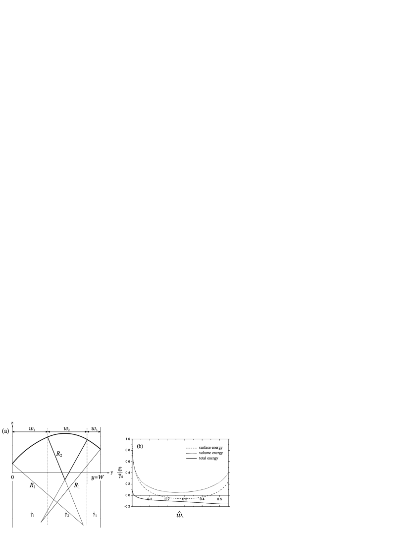
Figure 14: (a) Profile of the meniscus for the three-band configuration for $\hat{w}_{2}=0.45$ and $\hat{w}_{1}=0.4$, with contact angles $\phi_{1}=140^{\circ}$ and $\phi_{2}=130^{\circ}$, in which the outer bands have one shear rate $\dot{\gamma}_{1}$ and the inner band has a different shear rate. Normal stress balance ensures that the two outer bands have equal radii of curvature. The width $w_{2}$ of the inner band is given by $\hat{w}_{2}=(\dot{\gamma}_{\textrm{app}}-\dot{\gamma}_{1})/(\dot{\gamma}_{2}-\dot{\gamma}_{1})$. (b) Energy as a function of $\hat{w}_{1}$ showing the separate contributions from surface tension (surface) and pressure (volume). The stable configuration occurs for $\hat{w}_{1}\approx 0.52$.

C.2 Meniscus Integrity

The conditions for integrity of the surface, $h^{\prime}(w_{1})<\infty$ and $h^{\prime}(w_{1}+w_{2})<\infty$, lead to (from Eqs. 35)

$$\left|\left(1-\hat{w}_{1}\right)\cos\phi_{1}-\hat{w}_{1}\cos\phi_{2}-\hat{w}_{1}\hat{w}_{2}A\right|<1,$$ (36a)

$$\left|\left[1-\left(\hat{w}_{1}+\hat{w}_{2}\right)\right]\cos\phi_{1}-(\hat{w}_{1}+\hat{w}_{2})\cos\phi_{2}+\hat{w}_{2}\left[1-\left(\hat{w}_{1}+\hat{w}_{2}\right)\right]A\right|<1.$$ (36b)

These conditions apply at both interfaces of the central high shear rate band, and must be satisfied simultaneously for the meniscus to maintain integrity. The contact angles $\phi_{1}$, $\phi_{2}$ and the distortion parameter $A$ are properties of the fluid, while the width of the high shear rate band $w_{2}$ is determined by the applied shear rate.

Although a symmetric solution $w_{1}=w_{3}$ is appealing, we will consider the more general case where the two low shear rate bands need not be the same size. We will see that a simple stability analysis can lead to symmetry breaking to a non-symmetric band configuration. As has already been mentioned, stability should strictly be determined by dynamical considerations. However, since we are only treating the mechanics of the meniscus, we will study the three band configuration by constructing an energy function, which roughly corresponds to the work needed to establish an interface, and whose gradient specifies a generalized force that should vanish for mechanical stability.

The mechanical energy of the surface, per unit length in the flow direction, is given by

$${\cal E}(w_{1},w_{2},A,\phi_{1},\phi_{2})=\gamma_{s}\int_{0}^{W}\sqrt{1+h^{\prime 2}}\;\text{d}y\;-\;\Delta p\int_{0}^{W}h\;\text{d}y\;,$$ (37)

which comprises the surface tension and the work done in deforming against the pressure differences across the interface. We take ${\cal E}=0$ at the onset of banding. For a given width of the high shear rate band $w_{2}$ we determine the position of the band by minimising ${\cal E}$ with respect to $w_{1}$. We will only consider the equal contact angle case, $\phi_{1}=\phi_{2}=\phi$. Stable configurations are defined as those for which the energy function ${\cal E}$ is a local minimum with respect to changing the sizes $w_{1}$ and $w_{2}$ of the two outer shear bands at fixed $w_{2}$.

C.3 Different three-band configurations

Three configurations of the three band model minimize the energy, as demonstrated in Figs. 15.

1. central high shear rate band ($w_{1}=w_{3}$);

2. off center high shear rate band ($w_{1}\neq w_{3}$);

3. collapsed low shear rate band ($w_{1}=0$, or $w_{3}=0$), corresponding to two shear bands.

We can show that, for equal angles, there will be an extremum at $w_{1}=\frac{1}{2}(1-w_{2})$. The high shear rate band remains central so long as $\displaystyle{\frac{\partial^{2}{\cal E}}{\partial w_{1}^{2}}\Bigg{|}_{\frac{1}{2}(1-w_{2})}}\!\!\!\!\!\!\!\!\!\geq 0$. Equality defines $w^{\ast}_{2}$, so that the condition for stability is $w_{2}<w^{*}_{2}$ where $w^{*}_{2}$ satisfies

$$\frac{1}{\sqrt{1-\left(\frac{w_{2}^{*}}{2R_{2}}\right)^{2}}}-\left[1+\frac{A}{2\cos\phi}\frac{w_{2}^{*}}{W}\frac{R_{1}}{R_{2}}\right]+\left(\frac{R_{1}}{R_{2}}\right)\frac{\sqrt{1-\left(\frac{w_{2}^{*}}{2R_{2}}\right)^{2}}}{\sqrt{1-\left(\cos\phi\>\frac{w_{2}^{*}}{W}\right)^{2}}}=0,$$ (38)

together with the integrity conditions of equation (36). Further, for given distortion parameter $A$ and high shear rate band width $w_{2}$, a three band configuration may satisfy the integrity conditions of Eq. (36). At a slightly greater value of $w_{2}$ (or applied shear rate) the three band configuration becomes unstable and the fluid collapses into a two-band states, with integrity governed by equation (13).

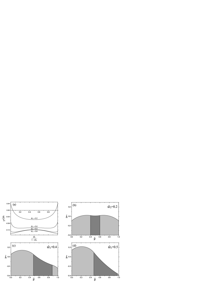
Figure 15: Total energy curves (a) and mensci shapes (b,c,d) for distortion parameter $A=-3.5$ and contact angle $\phi=130^{\circ}$. For widths $\hat{w}_{2}<0.343$ of the high shear rate bands (a), the central high shear rate band is stable. For $\hat{w}_{2}>0.343$ the high shear rate band is no longer stable at the central position but stabilises such that there is a wide low shear rate band and a narrow low shear rate band close to the plate (c,d). For $\hat{w}_{2}>0.579$ the fluid collapses into the two band configuration. The meniscus profiles are shown for $\hat{w}_{2}=0.2,0.4,0.5$, and the complete set of states for all contact angles is shown in Fig. 16.

Fig. 15 shows the energy curves and some meniscus shapes for the distortion parameter $A=-3.5$ and equal contact angles $\phi=130^{\circ}$, as a function of increasing the width of the central high shear rate band $\hat{w}_{2}$. For $\hat{w}_{2}/(1-\hat{w}_{2})=0.5$ the low shear material splits into two equal size bands surrounding the high shear rate band. Upon increasing $\hat{w}_{2}$ the symmetric three band configuration becomes unstable to an asymmetric configuration (for $\hat{w}_{2}>0.343$), and finally unstable to a two band configuration when the energy minima lie at either $\hat{w}_{1}=0$ or $\hat{w}_{1}=1-\hat{w}_{2}$.

Fig. 16 shows all loci of states whose meniscus integrity we can estimate using this method for $A=-3.5$. This figure shows the regions, in Fig. 6, in which two bands fracture at different ends of the stress plateau depending on whether the contact angle is closer to wetting or non-wetting angles. In addition, there are accompanying regions in which the inner of three bands is either symmetric or non-symmetric. In this particular example, the larger contact angles ($\phi>90^{\circ}$) correspond to a central high shear rate band, while the smaller contact angles ($\phi<90^{\circ}$) correspond to a central low shear rate band. There are four distinct classes of regions of for which the meniscus retains integrity: (1) two bands, (2) three bands with a central symmetric band, (3) either three symmetric bands or two bands, or (4) either three asymmetrically distributed bands or two bands. In the last two cases where two band configurations allow meniscus integrity we expect factors such as flow history, flow geometry (e.g. cylindrical Couette vs cone and plate) and boundary conditions to determine the selected configuration.

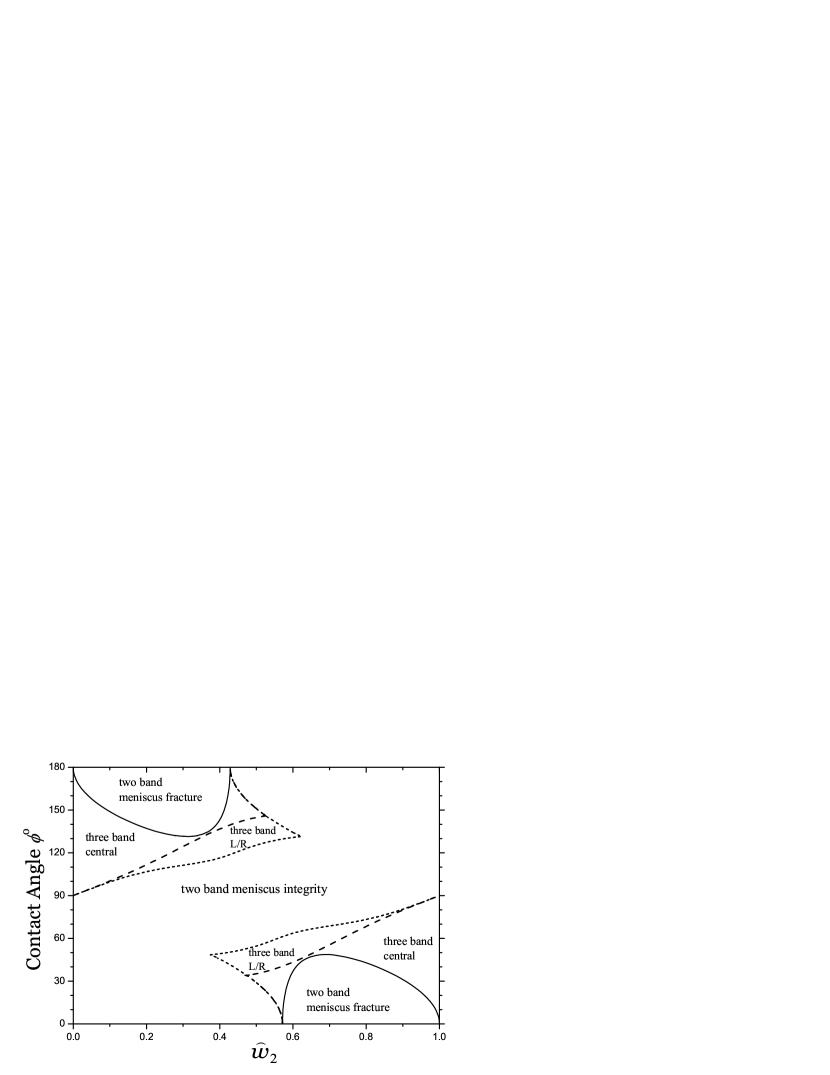
Figure 16: Integrity diagram for $A=-3.5$, show regions in which two or three bands allow meniscus integrity as a function of contact angle and the fraction of material $\hat{w}_{2}$ in the middle band. For $\phi>90^{\circ}$ ($\phi<90^{\circ}$) the central band adopts the high (low) shear rate.

Britton and Callaghan (1999) found the central high shear rate band to be stable and to increase in width as the applied shear rate increased (Fig. 17). At $\dot{\gamma}=7\;\text{s}^{-1}$ the high shear rate band is stable in a central position consistent with Fig. 15b, while at $\dot{\gamma}=10.7\;\text{s}^{-1}$ the high shear rate band is no longer central but in an off-center stable position consistent with Fig. 15c. This would be consistent with the state diagram in Fig. 16, for $\phi\gtrsim 120^{\circ}$.

Figure 17: NMR images of a worm-like micellar solution undergoing shear banding in a cone-and-plate rheometer (image from Fig. 10 Britton and Callaghan (1999)). At an applied shear rate of $\dot{\gamma}=7\;\text{s}^{-1}$ the high shear rate band, appearing as white/black, is stable and central. This would correspond to Figure (15b). At the higher applied shear rate $\dot{\gamma}=10.7\;\text{s}^{-1}$, the high shear rate band is stable but no longer central but positioned close to the moving cone. This corresponds to Figure (15c). At even higher shear rates the material was expelled from the cell.

C.4 Summary

In summary, we find the following results for three bands:

1. Three bands are stable in a subspace of the the parameter space, for a range of contact angles. This stability region starts with an infinitesimally small central band, and continues until the central band becomes too large, after which only a conventional two band state is possible.

2. The stable central band is the high (low) shear rate branch when the contact angle is closer to $180^{\circ}(0^{\circ})$.

3. The central of the three bands is symmetric for smaller central bands, but is destabilized towards an off-center configuration for wider central bands, for a range of contact angles.

4. In some regions of the phase space two-band and three-band states are simultaneously stable; in other regions the two band state is unstable, in principle towards three band states. This may explain some of the experiments of Britton and Callaghan (1997), in which three band states are found.

5. We are not able to assess the relative stability of two or three band states, and we speculate that this is determined by factors such as initial conditions, boundary conditions, and the degree of curvature in the flow. For example, the highly curved flow of a wide gap Couette rheometer may have a strong preference for the two band state, as it also leads to a preference for inducing the high shear rate phase next to the inner cylinder where the shear stress is highest (Radulescu and Olmsted, 2000; Adams, Fielding, and Olmsted, 2008).

References

- Adams, Fielding, and Olmsted (2008) Adams, J. M., Fielding, S. M., and Olmsted, P. D., “The interplay between boundary conditions and flow geometries in shear banding: hysteresis, band configurations, and surface transitions,” J. Non-Newt. Fl. Mech 151, 101–118 (2008).
- Adams and Olmsted (2009a) Adams, J. M. and Olmsted, P. D., “Adams and Olmsted reply:,” Phys. Rev. Lett. 103, 067801 (2009a).
- Adams and Olmsted (2009b) Adams, J. M. and Olmsted, P. D., “Nonmonotonic models are not necessary to obtain shear banding phenomena in entangled polymer solutions,” Phys. Rev. Lett. 102, 219802 (2009b).
- Akers and Belmonte (2006) Akers, B. and Belmonte, A., “Impact dynamics of a solid sphere falling into a viscoelastic micellar fluid,” J. Non-Newt. Fl. Mech. 135, 97–108 (2006).
- Bascom, Cottington, and Singleterry (1964) Bascom, W. D., Cottington, R. L., and Singleterry, C. R., “Contact angle, wettability, and adhesion,” (American Chemical Society, 1964) Chap. Dynamic Surface Phenomena, pp. 355–379.
- Berret (2005) Berret, J.-F., “Rheology of wormlike micelles: equilibrium properties and shear banding transition,” in Molecular Gels, edited by R. G. Weiss and P. Terech (Springer, Dordrecht, 2005) pp. 235–275.
- Berret, Porte, and Decruppe (1997) Berret, J. F., Porte, G., and Decruppe, J. P., “Inhomogeneous shear flows of wormlike micelles: a master dynamic phase diagram,” Phys. Rev. E 55, 1668–1676 (1997).
- Berret, Roux, and Porte (1994) Berret, J. F., Roux, D. C., and Porte, G., “Isotropic-to-nematic transition in wormlike micelles under shear,” J. Phys. II (France) 4, 1261–1279 (1994).
- Bird, Armstrong, and Hassager (1987) Bird, R. B., Armstrong, R. C., and Hassager, O., Dynamics of Polymeric Liquids (John Wiley and Sons, 1987).
- Boukany and Wang (2007) Boukany, P. E. and Wang, S.-Q., “A correlation between velocity profile and molecular weight distribution in sheared entangled polymer solutions,” J. Rheol. 51, 217 (2007).
- Boukany and Wang (2009) Boukany, P. E. and Wang, S.-Q., “Shear banding or not in entangled DNA solutions depending on the level of entanglement,” J. Rheol. 53, 73 (2009).
- Brandrup and Immergut (1989) Brandrup, J. and Immergut, E. H., Polymer Handbook, 3rd ed. (Wiley, New York, 1989).