Single-magnet rotary flowmeter for liquid metals

Abstract

We present a theory of single-magnet flowmeter for liquid metals and compare it with experimental results. The flowmeter consists of a freely rotating permanent magnet, which is magnetized perpendicularly to the axle it is mounted on. When such a magnet is placed close to a tube carrying liquid metal flow, it rotates so that the driving torque due to the eddy currents induced by the flow is balanced by the braking torque induced by the rotation itself. The equilibrium rotation rate, which varies directly with the flow velocity and inversely with the distance between the magnet and the layer, is affected neither by the electrical conductivity of the metal nor by the magnet strength. We obtain simple analytical solutions for the force and torque on slowly moving and rotating magnets due to eddy currents in a layer of infinite horizontal extent. The predicted equilibrium rotation rates qualitatively agree with the magnet rotation rate measured on a liquid sodium flow in stainless steel duct.

I Introduction

Flow rate measurements of liquid metals are required in various technological processes ranging from the cooling of nuclear reactors to the dosing and casting of molten metals.Cha-etal03 Electromagnetic flowmeters are essential in the diagnostics and automatic control of such processes. A variety of electromagnetic flowmeters have been developed starting from the late 1940s and described by Shercliff.Sher62 The standard approach is to determine the flow rate by measuring the potential difference induced between a pair of electrodes by a flow of conducting liquid in the magnetic field.Bev70 ; Hemp91 This approach is now well developed and works reliably for common liquids like water,Fu-etal10 but not so for liquid metals. Major problem in molten metals, especially at elevated temperatures, is the electrode corrosion and other interfacial effects, which can cause a spurious potential difference between the electrodes.

The electrode problem is avoided by contactless eddy-current flowmeters, which determine the flow rate by sensing the flow-induced perturbation in an applied magnetic field.Feng75 ; SGG04 The main problem with this type of flowmeters is the weak field perturbation which may be caused not only by the flow. We showed recently that the flow-induced phase shift of AC magnetic field is more reliable for flow rate measurements than the amplitude perturbation.PBG10

Another contactless techniques for flow rate measurements in liquid metals is the so-called magnetic flywheel invented by Shercliff,Sher60 who prescribes a “plurality” of permanent magnets distributed equidistantly along the circumference of a disk, which is mounted on an axle and placed close to a tube carrying the liquid metal flow. The eddy currents induced by the flow across the magnetic field interact with the magnets by entraining them, which makes the disk rotate with a rate proportional to that of the flow. This type of flowmeter, described also in the textbook by ShercliffSher62 and extensively used by Bucenieks,Buc02 ; Buc05 was recently successfully reembodied under the name of the Lorentz force velocimetry (LFV).TVK06

Recently, we suggested an alternative and much more compact design of such a flowmeter, which conversely to Shercliff’s flywheel uses just a single magnet mounted on the axle it can freely rotate around and magnetized perpendicularly to it.GPBBGB-09 We also introduced a basic mathematical model and presented first experimental implementation of this type of flowmeter.PBG09 When such a magnet is placed properly at a tube with the liquid metal flow, it starts to revolve similarly to Shercliff’s flywheel. But in contrast to the latter, which is driven by the electromagnetic force acting on separate magnets, the single magnet is set into rotation only by the torque. This driving torque is due to the eddy currents induced by the flow across the magnetic field. As the magnet starts to rotate, additional eddy currents are induced, which brake the rotation. An equilibrium rotation rate is attained when the braking torque balances the driving one, and this rate depends only on the flow velocity and the flowmeter arrangement, whereas it is independent of the electromagnetic torque itself. Thus, the equilibrium rotation rate is affected neither by the magnet strength nor by the electrical conductivity of the liquid metal provided that the friction on the magnet is negligible. This a major advantage of the single-magnet rotary flowmeter over the LFV approach, which relies on direct force measurements.TVKZ-07

In this paper, we present an extended theory of the single-magnet rotary flowmeter and compare it with experimental results. Two limiting cases of long and short magnets are analyzed using linear-dipole and single-dipole approximations. We obtain simple analytic solutions for the force and torque on slowly moving and rotating magnets due to eddy currents in the layers of infinite horizontal extent and arbitrary depth. This allows us to find the equilibrium rotation rate of the magnet at which the torques due to the translation and rotation balance each other. We also consider an active approach, where the force on the magnet is used to control its rotation rate so that the resulting force vanishes. This rotation rate, similarly to the equilibrium one, is proportional to the layer velocity and independent of its conductivity and the magnet strength.

The torque on a magnetic dipole rotating about an axis normal to a thin sheet has been calculated by Smythe using an original receding image method.Smythe-50 Reitz uses this method to calculate the lift and drag forces on the coils of various geometries moving with constant velocity above a conducting thin plate.Reitz-70 The lift force, which at high speeds approaches the force between the coil and its image located directly below it, varies as the velocity squared in the low-speed limit considered in this paper. The drag force is found to vary inversely and directly with the velocity at low and high speeds, respectively. Palmer finds analytical expressions for the eddy current forces on a circular current loop moving with a constant velocity parallel to a thin conducting sheet.Palmer-04 The force on a rectangular coil moving above a conducting slab has been calculated numerically by Reitz and Davis using the Fourier transform method.Reitz-Davis72 The same problem for the magnetic dipole of arbitrary orientation placed next to a thin slowly moving slab is addressed by Kirpo et al. KBT10 The force and torque on a transversely oriented dipole above a slowly moving plane layer of arbitrary thickness has been found analytically in the context of the LFV.TVKZ-07 Fast computation of forces on moving magnets are of interested also for the eddy current force testing techniques.ZiBr-10

This paper is organized as follows. The following section presents two simple mathematical models of the single-magnet rotary flowmeter, which are used to calculate analytically the force and torque on the magnets moving and rotating slowly above a layer of infinite lateral extent. The limits of long and short magnets, which are approximated by linear and point dipoles, are considered in Secs. II.2 and II.3, respectively. Section III presents the flowmeter implementation details and test results. The paper is concluded by a summary in Sec. IV.

II Theory

II.1 Formulation of problem

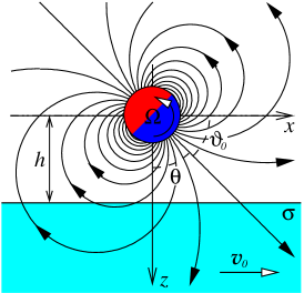
Figure 1: Schematic view of the single-magnet rotary flowmeter with the $y$-axis directed out of the plane of figure.

Consider a horizontally unbounded planar layer of electrical conductivity $\sigma$ occupying the lower half-space and moving as a solid body with a constant velocity $\mbox{\boldmath$v$}_{0}$ parallel to a permanent magnet placed at a distance $h$ above its surface and rotating with a constant angular velocity $\Omega$ around an axis parallel to the surface and perpendicular to $\mbox{\boldmath$v$}_{0}.$ Velocities are assumed sufficiently low for the magnetic field of induced currents to be negligible compared to the field of the magnet. The origin of Cartesian coordinates is set at the center of the magnet with the $x,$ $y$ and $z$ axis directed along $\mbox{\boldmath$v$}_{0}=v\mbox{\boldmath$e$}_{x},$ $\mbox{\boldmath$\Omega$}=\Omega\mbox{\boldmath$e$}_{y},$ and downward normally to the surface, respectively, as shown in Fig. 1. In the following, two limiting cases will be considered in which the magnet will be assumed either much longer or much shorter than $h.$

II.2 Linear-dipole model for a long magnet

We start with a long cylinder magnetized perpendicularly to its axis about which it can freely rotate.PBG09 In this case, the magnetic field is approximated by that of a two-dimensional (linear) dipole with the vector potential $\mbox{\boldmath$A$}\left(\mbox{\boldmath$r$}\right)=\mbox{\boldmath$e$}_{y}A\left(\mbox{\boldmath$r$}\right),$ which has only the $y$-component

$$A\left(\mbox{\boldmath$r$}\right)=\frac{\mu_{0}}{2\pi}\frac{\mbox{\boldmath$\bar{m}$}\cdot\mbox{\boldmath$r$}}{r^{2}}=\frac{\mu_{0}}{2\pi}\frac{\bar{m}\cos(\vartheta-\vartheta_{0})}{r},$$ (1)

where $\mu_{0}=4\pi\times 10^{-7}\,H/m$ is the vacuum permeability and $\bar{m}$ is the linear dipole moment, which is perpendicular to $\mbox{\boldmath$e$}_{y}$ and directed at the angle $\vartheta_{0}$ from the positive $x$ axis; $r$ is the radius vector from the magnet axis, and $r=\left|\mbox{\boldmath$r$}\right|$ and $\vartheta$ are the cylindrical radius and the polar angle in the cylindrical coordinates around the $y$-axis. The magnetic field of linear dipole is

$$\mbox{\boldmath$B$}=\mbox{\boldmath$\nabla$}\times\mbox{\boldmath$A$}=-\mbox{\boldmath$e$}_{y}\times\mbox{\boldmath$\nabla$}A.$$ (2)

Eddy currents are induced by two effects: the translation of the layer and the temporal variation of the magnetic field due to its rotation. The latter vanishes in the co-rotating frame of reference, where the magnetic field is stationary, while the layer appears to move with the resulting velocity $\mbox{\boldmath$v$}=\mbox{\boldmath$v$}_{0}+\mbox{\boldmath$v$}_{1},$ which contains also an apparent rotational motion of the layer $\mbox{\boldmath$v$}_{1}=-\mbox{\boldmath$\Omega$}\times\mbox{\boldmath$r$}$ opposite to that of the magnet. The density of eddy currents is given by Ohm’s law for a moving medium

$$\mbox{\boldmath$j$}=\sigma(-\mbox{\boldmath$\nabla$}\varphi+\mbox{\boldmath$v$}\times\mbox{\boldmath$B$})$$ (3)

where $\varphi$ is the electric potential. In this case, no electric potential is induced because the e.m.f., $\mbox{\boldmath$v$}\times\mbox{\boldmath$B,$}$ is both solenoidal and tangential to the surface. If the induced magnetic field is negligible as originally assumed, eddy currents can be represented as the superposition

$$\mbox{\boldmath$j$}=(j_{0}+j_{1})\mbox{\boldmath$e$}_{y},$$

where $j_{0}=-\sigma\mbox{\boldmath$v$}_{0}\cdot\mbox{\boldmath$\nabla$}A$ and $j_{1}=-\sigma\mbox{\boldmath$v$}_{1}\cdot\mbox{\boldmath$\nabla$}A$ are the currents induced by the translation and rotation, respectively.

It is important to note that in the approximation under consideration with a fixed magnetic field distribution, eddy currents are determined only by the instantaneous velocities. Besides that eddy currents are coplanar to the surface and, thus, mutually independent over the depth of the layer. Consequently, a layer of finite thickness may be represented as a semi-infinite one with zero velocity at $z>h_{2},$ where $h_{2}$ is the distance of the lower boundary of finite-thickness layer from the magnet. This, in turn, is equivalent to the superposition of two semi-infinite layers with the second layer at $z>h_{2}$ moving oppositely to the first one at $z>h_{1}$ so that the resulting velocity vanishes at $z>h_{2}.$ In the following, this approach allows us to construct the solution for a finite-thickness layer by taking the difference of two half-space solutions, which is subsequently denoted by $\left[X\right]_{h_{1}}^{h_{2}},$ where $X$ stands either for the force or the torque due to the eddy currents in a half-space. Moreover, by the same arguments, this approach can easily be extended to $z$-dependent velocity distributions $v(z)$, for which general solution can be constructed as a superposition of solutions for thin layers moving with various velocities given by $\int v(z)\partial_{z}X\,\textrm{d}z,$ where $\partial_{z}X=\left[X\right]_{h_{1}}^{h_{2}}/\left[z\right]_{h_{1}}^{h_{2}}$ for $h_{2}\rightarrow h_{1}=z$ and $v=1.$

The linear force density experienced by an infinitely long magnet due to the layer translation, which according to the momentum conservation law is opposite to that acting upon the layer itself, can be written as $-\int_{S}\mbox{\boldmath$j$}_{0}\times\mbox{\boldmath$B$}\,\textrm{d}s=F_{0}\mbox{\boldmath$e$}_{x},$ where the integral is taken over the $xz$-cross-section of the layer. The $y$-component of force is absent due to the $y\rightarrow-y$ reflection symmetry. In the low-speed limit under consideration, when force varies linearly with the velocity, there is also no $z$-component of force. This is the case because according to the linearity $\mbox{\boldmath$F$}\rightarrow-\mbox{\boldmath$F$}$ when $\mbox{\boldmath$v$}_{0}\rightarrow-\mbox{\boldmath$v$}_{0},$ while the latter transformation is equivalent to the rotation of the coordinate system by $180^{\circ}$ around the $z$-axis, which leaves the $z$-components invariant. In polar coordinates with the surface defined by $r_{1}=h/\sin\vartheta,$ we obtain

$$F_{0}=-\frac{\mu_{0}^{2}\bar{m}^{2}\sigma v}{4\pi^{2}}\int_{\pi}^{2\pi}\cos^{2}(2\vartheta-\vartheta_{0})\int_{r_{1}}^{\infty}\frac{\textrm{d}r}{r^{3}}\,\textrm{d}\vartheta=\frac{\mu_{0}^{2}\bar{m}^{2}\sigma v}{32\pi h^{2}}.$$ (4)

The linear torque density, which because of the aforementioned symmetries has only the $y$-component, can be found as $-\int_{S}\mbox{\boldmath$r$}\times\mbox{\boldmath$j$}_{0}\times\mbox{\boldmath$B$}\,\textrm{d}s=M_{0}\mbox{\boldmath$e$}_{y},$ where

$$M_{0}=\frac{\mu_{0}^{2}\bar{m}^{2}\sigma v}{4\pi^{2}}\int_{\pi}^{2\pi}\cos(2\vartheta-\vartheta_{0})\sin(\vartheta-\vartheta_{0})\int_{r_{1}}^{\infty}\frac{\textrm{d}r}{r^{2}}\,\textrm{d}\vartheta=\frac{\mu_{0}^{2}\bar{m}^{2}\sigma v}{16\pi h}.$$ (5)

The linear force density due to the rotation, defined by $-\int_{S}\mbox{\boldmath$j$}_{1}\times\mbox{\boldmath$B$}\,\textrm{d}s=F_{1}\mbox{\boldmath$e$}_{x},$ is found as

$$F_{1}=\sigma\int_{S}(\mbox{\boldmath$e$}_{x}\cdot\mbox{\boldmath$\nabla$}A)(\mbox{\boldmath$v$}_{1}\cdot\mbox{\boldmath$\nabla$}A)\,\textrm{d}s=-\frac{\mu_{0}^{2}\bar{m}^{2}\sigma\Omega}{16\pi h}.$$

The linear torque density due to the rotation, as that due to the translation above, has only the $y$-component

$$M_{1}=\sigma\int_{S}(\mbox{\boldmath$r$}\times\mbox{\boldmath$\nabla$}A)(\mbox{\boldmath$v$}_{1}\cdot\mbox{\boldmath$\nabla$}A)\cdot\textrm{d}\mbox{\boldmath$s$}=\frac{\mu_{0}^{2}\bar{m}^{2}\sigma\Omega}{4\pi^{2}}\int_{0}^{\pi}\sin^{2}(\vartheta-\vartheta_{0})\,\textrm{d}\vartheta\int_{r_{1}}^{\infty}\frac{\textrm{d}r}{r},$$ (6)

which is not defined for a semi-infinite layer because the last integral diverges. Nevertheless, expression (6) can still be evaluated for the layer of finite depth by substituting the infinite limit in the last integral by $r_{2}=h_{2}/\sin\vartheta,$ which results in

$$\frac{\mu_{0}^{2}\bar{m}^{2}\sigma\Omega}{8\pi}\ln\frac{h_{2}}{h_{1}}=\left[M_{1}\right]_{h_{2}}^{h_{1}}.$$ (7)

The solution above becomes unbounded as $h_{2}\rightarrow\infty$ and, thus, inapplicable to thick layers. This implies that for a half-space layer the induced magnetic field cannot be neglected however slow the rotation of magnet. The induced magnetic field is related to eddy currents by Ampere’s law $\mbox{\boldmath$j$}=\frac{1}{\mu_{0}}\mbox{\boldmath$\nabla$}\times\mbox{\boldmath$B$},$ which combined with expressions (2) and (3) leads to

$$\mu_{0}\sigma\mbox{\boldmath$v$}_{1}\cdot\mbox{\boldmath$\nabla$}A+\mbox{\boldmath$\nabla$}^{2}A=0.$$ (8)

As suggested by the external magnetic field (1), we search for the vector potential in the complex form

$$A(\mbox{\boldmath$r$})=\Re\left[\hat{A}(r)e^{i(\vartheta-\vartheta_{0})}\right].$$ (9)

Then Eq. (8) for the complex amplitude $\hat{A}$ takes the form

$$-i\mu_{0}\sigma\Omega\hat{A}=r^{-1}(r\hat{A}^{\prime})^{\prime}-r^{-2}\hat{A},$$ (10)

where the prime stands for the derivative with respect $r.$ The general solution of Eq. (10) can be written as $\hat{A}(r)=CK_{1}\left((1+i)r/d\right),$ where $C$ is an unknown constant to be determined by matching the induced and externally imposed magnetic fields; $K_{1}(z)$ is the modified Bessel function of the second kind,AbSt72 and $d=\sqrt{2/(\mu_{0}\sigma\Omega)}$ is the skin depth due to the rotation. At distances $r$ smaller than the skin depth $(r/d\ll 1),$ $\hat{A}\approx Cd/((1+i)r)$ is expected to approach the imposed field $\hat{A}=\mu_{0}\bar{m}/(2\pi r),$ which yields $C=(1+i)\mu_{0}\bar{m}/(2\pi d$) and

$$\hat{A}(r)=\frac{(1+i)\mu_{0}\bar{m}}{2\pi d}K_{1}\left((1+i)r/d\right).$$ (11)

Substituting expressions (9) and (11) into integral (6), the torque on the magnet can be represented as $M_{1}=\frac{\sigma\Omega}{2}\int_{0}^{\pi}I(r_{1}(\vartheta))\,\textrm{d}\vartheta,$ where $I(r)=\int_{r}^{\infty}\Re\left[\hat{A}^{*}\hat{A}\right]r\,\textrm{d}r$ and the asterisk denotes the complex conjugate. Using Eq. (10), after some algebra we obtain

$$I(r)=\frac{d^{2}}{2}r\Im\left[\hat{A}^{*}\hat{A}^{\prime}\right]=\left(\frac{\mu_{0}}{2\pi}\right)^{2}\Re\left[K_{0}((1+i)r/d)K_{1}((1-i)r/d)(1+i)r/d\right].$$

For the low rotation rates that satisfy $r/\delta\ll 1$, we obtain

$$I(r)\approx-\left(\frac{\mu_{0}}{2\pi}\right)^{2}\Re\left[\ln((1-i)r/d)+\gamma\right]=\left(\frac{\mu_{0}}{2\pi}\right)^{2}(\ln(2d/r)-\gamma),$$

where $\gamma=0.577215\ldots$ is Euler’s constant. Finally, taking into account that $r_{1}(\vartheta)=h_{1}/\sin\vartheta$ and $\int_{0}^{\pi}\ln(\sin\vartheta)\,\textrm{d}\vartheta=-\pi\ln 2,$ we obtain

$$M_{1}=\frac{\mu_{0}^{2}\bar{m}^{2}\sigma\Omega}{8\pi}\ln\frac{\tilde{d}}{h_{1}},$$ (12)

where $\tilde{d}=de^{-\gamma}$ is the effective skin depth, which owing to the low velocities under consideration is supposed to be large relative to $h_{1}$.

Now we can use the results above to find the magnet rotation rate depending on the velocity of layer. First, if the magnet rotates steadily without a significant friction, the torques due to the translation and rotation are at equilibrium: $\left[M_{0}+M_{1}\right]_{h_{2}}^{h_{1}}=0,$ which yields

$$\Omega=\frac{v}{2}\left(\frac{1}{h_{1}}-\frac{1}{h_{2}}\right)/\ln\frac{h_{2}}{h_{1}}.$$ (13)

Note that this equilibrium rotation rate $\Omega$ depends neither on the magnet strength nor on the layer conductivity unless $h_{2}\gtrsim\tilde{d}.$ In the latter case, the skin effect becomes important and, thus, $h_{2}$ has to be substituted by $\tilde{d}$ in the expression above.

The velocity of layer can be determined also in another way by measuring the force on the magnet, as in the LFV, to control the magnet rotation rate so that the resulting force vanishes, $\left[F_{0}+F_{1}\right]_{h_{2}}^{h_{1}}=0.$ This results in

$$\Omega=\frac{v}{2}\left(\frac{1}{h_{1}}+\frac{1}{h_{2}}\right),$$ (14)

which again depends linearly on the layer velocity, but does not depend on its conductivity or the magnet strength.

II.3 Single-dipole model for a short magnet

In the other limiting case of a short magnet, when the distance to the surface is large or at least comparable to the size of magnet, the latter can be considered as a dipole with the scalar magnetic potential

$$\Phi(\mbox{\boldmath$x$};\mbox{\boldmath$m$})=-\mbox{\boldmath$m$}\cdot\mbox{\boldmath$\nabla$}G(\mbox{\boldmath$x$}),$$ (15)

where $m$ is the dipole moment and $G(\mbox{\boldmath$x$})=(4\pi|\mbox{\boldmath$x$}|)^{-1}$ is the fundamental solution of Laplace’s equation, which satisfies $\mbox{\boldmath$\nabla$}^{2}G=-\delta(\mbox{\boldmath$x$})$ with the Dirac delta function on the r.h.s. In the following, we use simplified notation $\mbox{\boldmath$e$}_{m}\cdot\mbox{\boldmath$\nabla$}\equiv\partial_{m},$ where $\mbox{\boldmath$e$}_{m}=\mbox{\boldmath$m$}/m$ is the unit vector. Then the dipole magnetic field is given by $\mbox{\boldmath$B$}=-\mu_{0}(\mbox{\boldmath$\nabla$}\Phi-\delta(\mbox{\boldmath$x$})\mbox{\boldmath$m$}),$ where the last term is added to ensure the solenoidality of $B$ also at $\mbox{\boldmath$x$}=0.$ The associated dipole current distribution is

$$\mbox{\boldmath$J$}=\frac{1}{\mu_{0}}\mbox{\boldmath$\nabla$}\times\mbox{\boldmath$B$}=\mbox{\boldmath$\nabla$}\times\delta\mbox{\boldmath$m$},$$ (16)

which easily leads to the classical expressions for the force and torque used later on. In the following, we will be using also the spherical and cylindrical coordinates associated with the Cartesian ones in the usual way. As in the previous section, we change to the co-rotating frame of reference and consider the eddy currents due to translation and rotation separately.

II.3.1 Translation

For the translation with $\mbox{\boldmath$v$}_{0}=v\mbox{\boldmath$e$}_{x},$ the charge conservation $\mbox{\boldmath$\nabla$}\cdot\mbox{\boldmath$j$}=0$ applied to Eq. (3) results in Laplace’s equation for $\varphi_{0}$

$$\mbox{\boldmath$\nabla$}^{2}\varphi_{0}=0.$$ (17)

At the surface $z=h,$ the normal component of electric current vanishes:

$$\partial_{z}\varphi_{0}=vB_{y}.$$ (18)

In order to find the induced electric potential, firstly, it is important to notice that $B$ being a free-space magnetic field satisfies the Laplace equation itself. Consequently, the Cartesian components of $B$ satisfy this equation, too. Secondly, if $B_{y}$ in BC (18) satisfies Laplace’s equation, then

$$\varphi_{0}=v\int B_{y}\,\textrm{d}z=\mu_{0}mv\int\partial_{ym}^{2}G\,\textrm{d}z.$$ (19)

satisfies not only BC (18) but also Eq. (17) because the integration along a straight line, similarly to the differentiation, are interchangeable with the Laplacian. By the same argument, we can interchange integration and differentiation in expression (19), which yields

$$\varphi_{0}=\mu_{0}mv\partial_{ym}^{2}H,$$ (20)

where $H=\int G\,\textrm{d}z=\frac{1}{4\pi}(Q_{0}(\cos\theta)+q(r))$ and $Q_{0}(z)=\ln\sqrt{\frac{1+z}{1-z}}$ is the zeroth degree associated Legendre function of the second kind;AbSt72 $\theta$ is the spherical polar angle from the positive $z$-axis (see Fig. 1) and $r$ is the corresponding cylindrical radius. The “constant” of integration $q(r),$ which similarly to the first term $Q_{0}(\cos\theta)$ is supposed to be axisymmetric and also to satisfy the Laplace equation, is chosen to regularize $H$ at $r\rightarrow 0$ by removing the logarithmic singularity $Q_{0}=\ln\cot\frac{\theta}{2}\sim-\ln r$ for $z>0.$ This results in $q(r)=\ln r$ and

$$H=\frac{1}{4\pi}\left(Q_{0}(z/R)+\ln r\right),$$ (21)

where $R=|\mbox{\boldmath$x$}|$ is the spherical radius. For a transversal dipole $(\mbox{\boldmath$e$}_{m}=\mbox{\boldmath$e$}_{z}),$ considered also by Thess at al.TVKZ-07 , solution (20) reduces to

$$\varphi_{0}=\mu_{0}vm\partial_{y}G=-\mu_{0}v\Phi(\mbox{\boldmath$x$};m\mbox{\boldmath$e$}_{y}),$$ (22)

where the last term represents the magnetic potential of a dipole aligned with the $y$-axis. For a general dipole orientation, expression (21) substituted into solution (20) after some algebra yields

$$\varphi_{0}=\frac{\mu_{0}v}{4\pi}\left[\left(\frac{R-z}{Rr^{2}}-\frac{z}{2R^{3}}\right)(m_{x}\sin 2\vartheta-m_{y}\cos 2\vartheta)+\frac{2m_{z}r\sin\vartheta-m_{y}z}{2R^{3}}\right],$$ (23)

where $\vartheta$ is the azimuthal angle from the positive $x$-axis in the $xy$-plane.

The electric potential distribution (23) allows us to calculate the force acting upon the magnet, which, as noted above, is opposite to that acting upon the layer, i.e., $\mbox{\boldmath$F$}=-\int_{V}\mbox{\boldmath$f$}\,\textrm{d}V,$ where the integral of the Lorentz force density $\mbox{\boldmath$f$}=\mbox{\boldmath$j$}\times\mbox{\boldmath$B$}$ is taken over the layer volume $V.$ For the longitudinal force component, we obtain

$$F_{0,x} = \mu_{0}^{2}m^{2}\sigma v\int_{S}\left\{\frac{1}{2}\partial_{z}\left[(\partial_{ym}^{2}H)^{2}-(\partial_{m}G)^{2}\right]+\int_{h}^{\infty}(\partial_{xm}^{2}G)^{2}\,\textrm{d}z\right\}\,\textrm{d}s$$ (24)

$$= \frac{\mu_{0}^{2}\sigma v}{512\pi h^{3}}(3m_{x}^{2}+m_{y}^{2}+4m_{z}^{2}),$$

where the first integral is taken over the surface $S$ at $z=h$ and can be swapped with the second one over the layer depth. For a transversal dipole $(m_{x}=m_{y}=0)$, the expression above coincides with that of Thess et al.TVKZ-07 as well as with the result of ReitzReitz-70 for a thin sheet in the limit of a slowly moving dipole. As seen, the force is the strongest on a transversal dipole and reduces on longitudinal and spanwise dipoles by factors of $\frac{3}{4}$ and $\frac{1}{4}$, respectively. Thus, the force (24), in contrast to force (4) for a long magnet, varies with the dipole orientation in the $xz$-plane. On a horizontally inclined dipole $(m_{x}m_{y}\not=0)$, there is also a spanwise force component

$$F_{0,y} = \mu_{0}^{2}m^{2}\sigma v\int_{S}\left\{(\partial_{ym}^{2}H)(\partial_{xy}^{2}G)+\int_{h}^{\infty}(\partial_{xm}^{2}G)(\partial_{ym}^{2}G)\,\textrm{d}z\right\}\,\textrm{d}s$$ (25)

$$= \frac{\mu_{0}^{2}\sigma v}{256\pi h^{3}}m_{x}m_{y}.$$

But there is no vertical force whatever the dipole orientation:

$$F_{0,z}=\mu_{0}^{2}\sigma v\int_{h}^{\infty}\int_{S}(\partial_{xm}^{2}G)(\partial_{zm}^{2}G)\,\textrm{d}s\,\textrm{d}z=0.$$ (26)

This is consistent with the result of ReitzReitz-70 stating that in the low-speed limit the lift force is proportional to the velocity squared, while the approximation under consideration takes into account only the part of force proportional to the velocity.

Alternatively, the force and torque acting on dipole can be found using the associated current distribution (16) and the induced magnetic field $\mbox{\boldmath$b$},$ which lead straightforwardly to the classical expressionsJac98

$$F = \int_{\bar{V}}\mbox{\boldmath$J$}\times\mbox{\boldmath$b$}\,\textrm{d}^{3}\mbox{\boldmath$x$}=(\mbox{\boldmath$m$}\cdot\mbox{\boldmath$\nabla$})\mbox{\boldmath$b$},$$ (27)

$$M = \int_{\bar{V}}\mbox{\boldmath$x$}\times\mbox{\boldmath$J$}\times\mbox{\boldmath$b$}\,\textrm{d}^{3}\mbox{\boldmath$x$}=\mbox{\boldmath$m$}\times\mbox{\boldmath$b$},$$ (28)

where the integrals are taken over the space $\bar{V}$ above the layer. This is a bit longer but algebraically more straightforward approach, which will be pursued in the following.

In order to find the induced magnetic field $\mbox{\boldmath$b$},$ it is important to notice that solution (19) satisfies condition (18) not only at $z=h$ but at any $z.$ Thus, the $z$-component of the current is absent not only at the surface but throughout the whole layer. Then $\mbox{\boldmath$\nabla$}\cdot\mbox{\boldmath$j$}=0$ and $j_{z}\equiv 0$ imply

$$\mbox{\boldmath$j$}=\mbox{\boldmath$\nabla$}\times\psi\mbox{\boldmath$e$}_{z},$$ (29)

where $\psi$ is the electric stream function, whose isolines coincide with the eddy current lines. Substituting this expression into Eq. (3) and taking the $z$-component of the curl of the resulting equation, we obtain

$$(\mbox{\boldmath$\nabla$}^{2}-\partial_{z}^{2})\psi=-\sigma\mbox{\boldmath$e$}_{z}\cdot\mbox{\boldmath$\nabla$}\times(\mbox{\boldmath$v$}\times\mbox{\boldmath$B$}).$$ (30)

Note that in contrast to the electric potential in Eq. (17), no boundary conditions are required for $\psi$ at the surface. This is because, firstly, Eq. (30) contains no derivatives in $z$ and, secondly, the absence of the $z$-component of current at the surface is explicitly ensured by expression (29).

For translational motion with $\mbox{\boldmath$v$}_{0}=v\mbox{\boldmath$e$}_{x},$ the r.h.s of Eq. (30) takes the form $\sigma v\partial_{x}B_{z}=-\mu_{0}\sigma v\partial_{xz}^{2}\Phi,$ which by the same arguments as above satisfies Laplace’s equation and equals to $-\partial_{z}^{2}\psi_{0}$ with

$$\psi_{0}=-\mu_{0}m\sigma v\partial_{xm}^{2}H,$$ (31)

which satisfies the same equation and, thus, represents the solution of Eq. (30). For a transversal dipole $(\mbox{\boldmath$e$}_{m}=\mbox{\boldmath$e$}_{z}$), the general solution (31) simplifies to

$$\psi_{0}=-\mu_{0}m\sigma v\partial_{x}G=\mu_{0}\sigma v\Phi(\mbox{\boldmath$x$};m\mbox{\boldmath$e$}_{x}),$$ (32)

where the last term represents the magnetic potential of a longitudinal dipole. Thus, in this case, the eddy current lines coincide with the isolines of electric potential (23) rotated by $90^{\circ}$ about the $z$-axis. For a longitudinal dipole $(\mbox{\boldmath$e$}_{m}=\mbox{\boldmath$e$}_{x}),$ the comparison of solutions (31) and (20) shows that the eddy current lines and the electric potential isolines are swapped with the corresponding distributions induced by a spanwise dipole $(\mbox{\boldmath$e$}_{m}=\mbox{\boldmath$e$}_{y})$ and rotated by $90^{\circ}$ about the $z$-axis. For an arbitrarily oriented dipole, expression (21) substituted into the general solution (31) after some algebra yields

$$\psi_{0}=-\frac{\mu_{0}\sigma v}{4\pi}\left[\left(\frac{R-z}{Rr^{2}}-\frac{z}{2R^{3}}\right)(m_{x}\cos 2\vartheta+m_{y}\sin 2\vartheta)+\frac{2m_{z}r\cos\vartheta-m_{x}z}{2R^{3}}\right].$$ (33)

Figure 2 shows the isolines of the electric potential (23) and those of $\psi_{0},$ which represent the eddy current lines, in the $xy$-plane $(z=\mbox{const})$ for three basic dipole orientations along the $x$-, $y$- and $z$-axis. Note that the patterns are self-similar in the $xy$-plane with the characteristic length scaling directly with $z.$ Namely, these distributions are functions of spatial angles only, while according to (23) and (33) the magnitude of both $\varphi_{0}$ and $\psi_{0}$ falls off as $\sim z^{-2}.$

Figure 2: Isolines of the electric potential $\varphi_{0}$ (dashed) and of the stream function $\psi_{0}$ (solid) in the $xy$-plane, where the latter represent the eddy current lines, induced by translation in the magnetic field of the dipole aligned with the $x$- (a), $y$- (b), and $z$-axis (c).

In order to satisfy the solenoidality condition $\mbox{\boldmath$\nabla$}\cdot\mbox{\boldmath$b$}=0,$ the induced magnetic field is sought as $\mbox{\boldmath$b$}=\mbox{\boldmath$\nabla$}\times\mbox{\boldmath$a$},$ where $a$ is the vector potential, which is supposed to satisfy the Coulomb gauge $\mbox{\boldmath$\nabla$}\cdot\mbox{\boldmath$a$}=0.$ Then Ampere’s law leads to $\mbox{\boldmath$\nabla$}^{2}\mbox{\boldmath$a$}=-\mu_{0}\mbox{\boldmath$j$},$ which, in turn, results in $\mbox{\boldmath$a$}(\mbox{\boldmath$x$})=\mu_{0}\int_{V}\mbox{\boldmath$j$}(\mbox{\boldmath$x$}^{\prime})G(\mbox{\boldmath$x$}-\mbox{\boldmath$x$}^{\prime})\,\textrm{d}^{3}\mbox{\boldmath$x$}^{\prime}.$ Substituting expression (29) into the last integral, after some algebra we obtain $\mbox{\boldmath$a$}=\mu_{0}\mbox{\boldmath$\nabla$}\times\chi\mbox{\boldmath$e$}_{z},$ where

$$\chi(\mbox{\boldmath$x$})=\int_{V}\psi(\mbox{\boldmath$x$}^{\prime})G(\mbox{\boldmath$x$}-\mbox{\boldmath$x$}^{\prime})\,\textrm{d}^{3}\mbox{\boldmath$x$}^{\prime}$$

is the same as used by Thess et al.TVKZ-07 The previous expression implies that $\mbox{\boldmath$a$},$ similarly to its source $\mbox{\boldmath$j$},$ has no $z$-component. Then the induced magnetic field can be written as

$$\mbox{\boldmath$b$}=\mu_{0}\mbox{\boldmath$\nabla$}\times\mbox{\boldmath$\nabla$}\times\chi\mbox{\boldmath$e$}_{z}=\mu_{0}(\mbox{\boldmath$e$}_{z}\psi-\mbox{\boldmath$\nabla$}\phi),$$

where $\phi=-\partial_{z}\chi$ represents the scalar magnetic potential, which completely defines $b$ outside the layer, where $\psi=0.$ Further, using the tensor notation with the Einstein summation convention, expressions (27) and (28) can be represented in terms of $\chi$ as

$$F_{i} = \mu_{0}m_{j}\chi_{;ij3},$$ (34)

$$M_{i} = \mu_{0}\epsilon_{ijk}m_{j}\chi_{;k3},$$ (35)

where $\epsilon_{ijk}$ is the anti-symmetric tensor and the subscript after the semicolon denotes the differential with respect to the corresponding coordinate with indices $1,$ $2$ and $3$ standing for the $x,$$y$ and $z,$ directions, respectively. Taking into account the symmetry of $G(\mbox{\boldmath$x$}-\mbox{\boldmath$x$}^{\prime})$ with respect to the interchange of observation and integration points, the derivatives of $\chi$ at the dipole location $\mbox{\boldmath$x$}=0$ in expressions (34) and (35) are found as

$$\chi_{;ij} = \int_{V}\psi(\mbox{\boldmath$x$})G_{;ij}(\mbox{\boldmath$x$})\,\textrm{d}^{3}\mbox{\boldmath$x$},$$ (36)

$$\chi_{;ijk} = -\int_{V}\psi(\mbox{\boldmath$x$})G_{;ijk}(\mbox{\boldmath$x$})\,\textrm{d}^{3}\mbox{\boldmath$x$},$$ (37)

where

$$G_{;ij}(\mbox{\boldmath$x$}) = \frac{3x_{i}x_{j}-\delta_{ij}|\mbox{\boldmath$x$}|^{2}}{4\pi|\mbox{\boldmath$x$}|^{5}},$$

$$G_{;ijk}(\mbox{\boldmath$x$}) = -\frac{15x_{i}x_{j}x_{k}-3(\delta_{ij}x_{k}+\delta_{ik}x_{j}+\delta_{jk}x_{i})|\mbox{\boldmath$x$}|^{2}}{4\pi|\mbox{\boldmath$x$}|^{7}}.$$

Integrals (36) and (37) can be evaluated analytically using, for example, the computer algebra system Mathematica,Wolf96 which also allows us to carry out all other analytical transformations. In such a way, we firstly verify that Eq. (34) with expression (31) substituted into integral (37) indeed reproduces previous results (24), (25) and (26). Secondly, Eq. (35) with the same expression for $\psi_{0}$ substituted in integral (36) results in

$$\mbox{\boldmath$M$}_{0}=\frac{\mu_{0}^{2}\sigma v}{128\pi h^{2}}\left(-m_{x}m_{y}\mbox{\boldmath$e$}_{x}+(m_{x}^{2}+m_{z}^{2})\mbox{\boldmath$e$}_{y}-m_{y}m_{z}\mbox{\boldmath$e$}_{z}\right),$$ (38)

which for a transversal dipole again coincides with the results of Thess et al.TVKZ-07

II.3.2 Rotation

For a solid-body rotation with the velocity $\mbox{\boldmath$v$}_{1}=-\mbox{\boldmath$\Omega$}\times\mbox{\boldmath$x$},$ which appears in the co-rotating frame of reference, the charge conservation $\mbox{\boldmath$\nabla$}\cdot\mbox{\boldmath$j$}=0$ applied to Eq. (3) results in

$$\mbox{\boldmath$\nabla$}^{2}\varphi_{1}=-2\Omega B_{y},$$ (39)

while the vanishing of the normal current component at the surface $z=h$ requires

$$\partial_{z}\varphi_{1}=-\Omega zB_{y}.$$ (40)

In order to solve this problem, firstly, it is important to notice that since $\int B_{y}\,\textrm{d}z$ satisfies the Laplace equation,

$$\bar{\varphi}_{1} = \Omega z\int B_{y}\,\textrm{d}z=\mu_{0}m\Omega z\partial_{ym}^{2}H$$ (41)

is a particular solution to Eq. (39). Comparing expressions (41) and (23) shows that $\bar{\varphi}_{1}=(\Omega z/v)\varphi_{0},$ where $\varphi_{0}$ is given by solution (20). Searching for the solution as $\varphi_{1}=\bar{\varphi}_{1}+\tilde{\varphi}_{1},$ reduces Eq. (39) to the Laplace equation for $\tilde{\varphi}_{1},$ while BC (40) takes the form

$$\partial_{z}\tilde{\varphi}_{1}=-\mu_{0}m\Omega\partial_{ym}H.$$

By the usual arguments, we obtain

$$\tilde{\varphi}_{1}=-\mu_{0}m\Omega\partial_{ym}H_{1},$$ (42)

where $H_{1}=\int H\,\textrm{d}z=\frac{1}{4\pi}\left(RQ_{1}(\cos\theta)+z\ln r\right)=zH-R^{2}G$ and $Q_{1}(z)=zQ_{0}(z)-1$ is the first order associated Legendre function of the second kind.AbSt72 Using the expressions above, after some transformations we obtain

$$\varphi_{1} = -\mu_{0}\Omega\left(\mbox{\boldmath$e$}_{x}\cdot\mbox{\boldmath$m$}\times\mbox{\boldmath$\nabla$}H+ym\partial_{m}G\right)=$$ (43)

$$-\frac{\mu_{0}\Omega}{4\pi}\left[\frac{m_{z}(R^{3}-z^{3})\sin\vartheta}{R^{3}r}+\frac{(m_{x}\sin 2\vartheta-m_{y}\cos 2\vartheta)r^{2}-m_{y}(R^{2}+z^{2})}{2R^{3}}\right].$$

which is the electric potential in the co-rotating frame of reference.

Figure 3: Instantaneous isolines of the electric potential $\varphi_{1}$ (dashed) and of the stream function $\psi_{1}$ (solid), which represent the eddy current lines, induced by a solid-body rotation in the magnetic field of the dipole aligned with the $x$- (a), $y$- (b), and $z$-axis (c).

As before, condition (40) is satisfied not only at $z=h$ but any $z$ and, thus, the $z$-component of the current vanishes throughout the layer. Consequently, the electric current can again be expressed as (29) with $\psi_{1},$ for which Eq. (30) takes the form

$$(\mbox{\boldmath$\nabla$}^{2}-\partial_{z}^{2})\psi_{1}=\sigma\Omega(B_{x}+\mbox{\boldmath$e$}_{y}\cdot\mbox{\boldmath$r$}\times\mbox{\boldmath$\nabla$}B_{z}).$$ (44)

Since the r.h.s. of Eq. (44) satisfies the Laplace equation, after some algebra we obtain

$$\psi_{1} = -\sigma\Omega\left(\iint B_{x}\,\textrm{d}z^{2}+\mbox{\boldmath$e$}_{y}\cdot\mbox{\boldmath$r$}\times\mbox{\boldmath$\nabla$}\iint B_{z}\,\textrm{d}z^{2}-2\partial_{x}\iiint B_{z}\,\textrm{d}z^{3}\right)$$ (45)

$$= \mu_{0}\sigma\Omega\mbox{\boldmath$e$}_{y}\cdot\mbox{\boldmath$m$}\times\mbox{\boldmath$\nabla$}H=\frac{\mu_{0}\sigma\Omega}{4\pi}\left(\frac{m_{z}(R-z)\cos\vartheta-m_{x}r}{Rr}\right).$$

The eddy current lines in the $xy$-plane, which are the isolines of $\psi_{1},$ along with the isolines of the electric potential (43) are shown in Fig. 3. Again, the patterns are self-similar and scale directly with the distance $z$ from the dipole, while the magnitude of both $\psi_{1}$ and $\varphi_{1}$ falls off as $\sim z^{-1}.$ In contrast to the translation considered above, the eddy currents induced by rotation are time-dependent and vary periodically as the dipole orientation changes from the $x$- to the $z$-axis, which are shown in Figs. 3(a) and (c), respectively. Only the electric potential, but no current, is induced by a solid-body rotation when the dipole is aligned with the axis of rotation ($y$). In his case, when the magnetic field is symmetric about the axis of rotation, the induced e.m.f. is irrotational and, thus, compensated by the electric potential gradient, which equals to

$$-\mbox{\boldmath$v$}_{1}\times\mbox{\boldmath$B$}=-\Omega\rho\mbox{\boldmath$\epsilon$}\times\mbox{\boldmath$\nabla$}\times(A\mbox{\boldmath$\epsilon$})=-\Omega\mbox{\boldmath$\nabla$}(\rho A),$$ (46)

where $\rho=|\mbox{\boldmath$\Omega$}\times\mbox{\boldmath$x$}|/\Omega$ is the cylindrical radius from the axis of rotation, $\mbox{\boldmath$\epsilon$}=\mbox{\boldmath$\Omega$}\times\mbox{\boldmath$x$}/|\mbox{\boldmath$\Omega$}\times\mbox{\boldmath$x$}|$ is the azimuthal unity vector, and $A$ is the azimuthal component of the vector potential, which can be used to describe a general axially symmetric poloidal magnetic field. For the dipole field, we have

$$\mbox{\boldmath$A$}(\mbox{\boldmath$x$})=\mu_{0}\int_{\bar{V}}\mbox{\boldmath$J$}(\mbox{\boldmath$x$}^{\prime})G(\mbox{\boldmath$x$}-\mbox{\boldmath$x$}^{\prime})\,\textrm{d}^{3}\mbox{\boldmath$x$}^{\prime}=\mbox{\boldmath$m$}\times\mbox{\boldmath$\nabla$}G(\mbox{\boldmath$x$})=A(\mbox{\boldmath$x$})\mbox{\boldmath$\epsilon$},$$

where $J$ is the associated dipole current (16) and $A(\mbox{\boldmath$x$})=-|\mbox{\boldmath$m$}\times\mbox{\boldmath$x$}|G(\mbox{\boldmath$x$})/|\mbox{\boldmath$x$}|^{2}.$ Substituting this into expression (46) and equating it to the gradient of the electric potential $\varphi_{1},$ we obtain

$$\varphi_{1}=-\Omega\rho A=\frac{\mu_{0}m_{y}\Omega(R^{2}-y^{2})}{4\pi R^{3}},$$

which is the free-space electric potential in the co-rotating frame of reference shown in Fig. 3(b) and coinciding with (43) when $m_{x}=m_{z}=0.$ This potential vanishes in the laboratory frame of reference, where the magnetic field is invariant with respect to the rotation around the symmetry axis.

Further, using expression (45) for $\psi_{1}$ in integrals (36) and (37), which can be evaluated together with Eqs. (34) and (35) in the same way as for the translation in the previous section, we obtain

$$\mbox{\boldmath$F$}_{1} = \frac{\mu_{0}^{2}\sigma\Omega}{128\pi h^{2}}(-(m_{x}^{2}+m_{z}^{2})\mbox{\boldmath$e$}_{x}-m_{x}m_{y}\mbox{\boldmath$e$}_{y}+m_{x}m_{z}\mbox{\boldmath$e$}_{z}),$$ (47)

$$\mbox{\boldmath$M$}_{1} = \frac{\mu_{0}^{2}\sigma\Omega}{64\pi h}(2m_{x}m_{y}\mbox{\boldmath$e$}_{x}-(2m_{x}^{2}+m_{z}^{2})\mbox{\boldmath$e$}_{y}+m_{y}m_{z}\mbox{\boldmath$e$}_{z}).$$ (48)

The first point to note is that both the force and torque vanishes when dipole is aligned with the axis of rotation $(m_{x}=m_{z}=0),$ which, as discussed above, is due to the absence of eddy currents in this case. Secondly, the longitudinal $(x)$ component of force (47), in contrast to that due to the translation given by expression (24), is independent of the dipole orientation in the $xz$-plane and depends only on the magnitude of the dipole moment in this plane: $\bar{m}^{2}=m_{x}^{2}+m_{z}^{2}.$ Thirdly, there is also a non-zero transversal $(z)$ force, which in contrast to the longitudinal one is purely oscillatory and varies periodically with the dipole orientation in the $xz$-plane as $m_{x}m_{z}=\frac{1}{2}\bar{m}^{2}\sin 2\vartheta_{0},$ where $\vartheta_{0}$ is the poloidal angle of the dipole orientation in the $xz$-plane from the positive $x$-axis, which is the same as that for the linear dipole in expression (1) (see Fig. 1). Moreover, when dipole is inclined to the axis of rotation ($m_{x}m_{y}\not=0),$ also a spanwise $(y)$ force appears, which similarly to the transversal one alternates periodically around zero as $m_{x}m_{y}=\bar{m}m_{y}\cos\vartheta_{0}$ with the dipole rotation. As seen from expression (48), inclination also gives rise to alternating torque components around both the $x$- and $z$-axis. The $y$-component of torque, which is negative and, thus, opposing the rotation, has not only a constant but also an alternating part, which varies with the double frequency of rotation as $-(2m_{x}^{2}+m_{z}^{2})=-\frac{3}{2}\bar{m}^{2}\left(1-\frac{1}{3}\cos 2\vartheta_{0}\right).$

Figure 4: Instantaneous rotation rate (51) versus time (solid) and orientation (dashed) for a negligible inertia of the magnet.

Thus, in contrast to the long magnet in $\S$II.2, there is no steady rotation rate, which could balance the $y$-component of the constant torque (38) due to the translation. The variation of the magnet rotation rate in response to oscillatory torque is constrained by the inertia of magnet. For the oscillatory part of the rotation rate $\tilde{\Omega}$ to be negligible compared to the mean one $\bar{\Omega},$ we need

$$\frac{\tilde{\Omega}}{\bar{\Omega}}\sim\frac{M}{\bar{\Omega}^{2}I}\sim\frac{\mu_{0}^{2}m^{2}\sigma}{\bar{\Omega}Ih}\ll 1$$ (49)

where $I$ is the moment of inertia of magnet. If this condition is satisfied, the oscillatory component may be neglected in the balance of torques (38) and (48) around the axis of rotation, which is the $y$-axis. For a layer of finite thickness, this results in

$$\bar{\Omega}_{0}=\frac{v}{3}\left(\frac{1}{h_{1}}+\frac{1}{h_{2}}\right).$$ (50)

The expression above differs only by a factor of $\frac{2}{3}$ from result (14) for a long magnet in the case of a vanishing longitudinal force. In the opposite limit of a negligible inertia, the torque balance yields

$$\Omega=\bar{\Omega}_{0}/(1-\tfrac{1}{3}\cos 2\vartheta_{0}).$$ (51)

This instantaneous rotation rate $\Omega=\partial_{t}\vartheta_{0},$ which is shown in Fig. 4 versus both the time $t$ and orientation $\vartheta_{0},$ alternates between $\frac{3}{4}\bar{\Omega}_{0}$ and $\frac{3}{2}\bar{\Omega}_{0}$ of the mean value (50) $\bar{\Omega}_{0}=\left.\vartheta_{0}/t\right|_{t\rightarrow\infty}.$ The last relation follows from the integration of Eq. (51) as $\vartheta_{0}-\frac{1}{6}\sin 2\vartheta_{0}=\bar{\Omega}_{0}t,$ which also defines $\Omega$ parametrically versus $t$ in Fig. 4. Note that the oscillations of the rotation rate do not affect its mean value $\bar{\Omega}_{0},$ which is defined by (50) independently of condition (49).

Alternatively, when the magnet rotation rate is actively controlled so that to balance the longitudinal force (24) with the $x$-component of force (47), the instantaneous rotation rate is

$$\Omega=\partial_{t}\vartheta_{0}=\frac{\bar{\Omega}_{1}}{4\sqrt{3}}(7-\cos 2\vartheta_{0}),$$ (52)

where the temporal mean value

$$\bar{\Omega}_{1}=\frac{\sqrt{3}v}{2}\left(\frac{1}{h_{1}}+\frac{1}{h_{2}}-\frac{1}{h_{1}+h_{2}}\right)$$ (53)

follows from the solution of differential equation (52), which can be written as

$$\tan(\vartheta_{0}(t))=\frac{\sqrt{3}}{2}\tan(\bar{\Omega}_{1}t).$$

III Implementation and testing

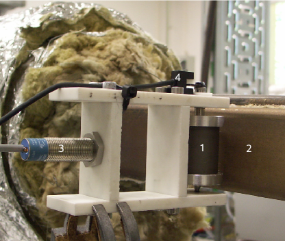
Figure 5: Single-magnet rotary flowmeter with a SmCo-type magnet (1) of $24\,\mbox{mm}$ and $35\,\mbox{mm}$ in diameter and height, respectively, installed at the side of a rectangular stainless steel duct (2) of $45\times 45\,\mbox{mm}^{2}$ in cross-section carrying the liquid sodium flow. The rotation rate is measured with an inductive magnetic proximity sensor (3) and also monitored with a photoelectric barrier sensor (4).

The laboratory model of the single-magnet flowmeter shown in Fig. 5 consists of a cylindrical SmCo-type permanent magnet with diameter $2R=24\,\mbox{mm}$ and height $L=35\,\mbox{mm}$, magnetized perpendicularly to its axis with $0.5\,\mbox{T}$ surface induction, which holds up to $230^{\circ}\mbox{C}.$ The magnet is mounted on a stainless steel axle held by a housing made of “MACOR” ceramic, which ensures a low mechanical friction and can withstand up to $800^{\circ}\mbox{C}.$

The flowmeter was tested on a sodium loop using about 90 liters of molten Na at $220^{\circ}\mbox{C}$ with the electrical conductivity of $9\times 10^{6}\,\mbox{S}\,\mbox{m}^{-1}.$ The flow was driven by a linear electromagnetic pump, which provided a maximum velocity of $1.5\,\mbox{m}\,\mbox{s}^{-1}$ at the flow rate of $3\,\mbox{l}\,\mbox{s}^{-1}$ in a stainless steel duct of $45\times 45\,\mbox{mm}^{2}$ cross-section.

The frequency of magnet rotation was determined with an inductive magnetic proximity sensor (SICK MM12-60APS-ZU0), which was fixed at the distance of $50\,\mbox{mm}$ perpendicularly to the side surface of magnet at its midheight as shown in Fig. 5. The sensor briefly switched off and then on again as the magnetic field along the axis of the sensor changed its direction. The frequency of sensor transition from the off to the on state, which happens twice per revolution, was measured with Keithley 2000 Multimeter using the reciprocal frequency counting techniques with the measurement gate time set to $1\,\mbox{s}.$ The frequency was also monitored with Tektronix TDS 210 oscilloscope. After changing the pump current, the flow was allowed to develop for $2\,\mbox{min},$ and then six measurements were taken with the intervals of approximately $30\,\mbox{s}.$ The standard deviation in the measured rotation frequencies was typically a few tenths of Hz.

The rotation rates measured at two gap widths between the magnet and the duct are shown in Fig. 6(a) depending on the average sodium velocity, which was determined using Ultrasonic Doppler VelocimetryEck-etal-11 with the resolution of $1\,\mbox{cm}\,\mbox{s}^{-1}.$EG-02 Although the rotation rate is seen to increase as the magnet is approached to the duct and to vary nearly linearly with the flow velocity in agreement with the theory, the linear fit shows a certain zero offset. Obviously, there is some opposing force, which has to be overcome for the rotation to start. This requires the flow velocity of at least $0.2\,\mbox{m}\,\mbox{s}^{-1}.$ First, such an opposing force is caused by the dry friction in bearings. Second, the magnet is oriented by the Earth’s magnetic field, which has a stronger effect than the friction and also has to be overcome for the rotation to start. Third, even stronger effect is caused by the stainless steel walls of the duct, which are weakly ferromagnetic.WebFaj-98 The magnet, when approached to the duct, was observed to turn with the dipole moment perpendicular to the wall. It is also important to note that the magnet, when turned by hand away from the equilibrium orientation, returned to it monotonically without oscillations. This implies the inertia of magnet to be small relative to the electromagnetic drag force. Thus, the inertia cannot significantly contribute to the overcoming of the orienting torque due to the wall magnetization. However, when magnet rotates slowly, the orienting torque causes the rotation rate to fluctuate, which shows up as an increased scatter in the measured values seen in Fig. 6 at low flow velocities.

When the zero offset is removed and the remaining rotation rate is multiplied by the distance $h=R+d_{w}+d$ between the magnet axis and the liquid metal, where $R=12\,\mbox{mm}$ is the magnet radius and $d_{w}=3\,\mbox{mm}$ is the thickness of stainless steel wall, we obtain the relative rotation rate $k=\Omega h/v,$ which represents a rescaled slope coefficient for Fig. 6(a) and is plotted in Fig. 6(b) versus the velocity. The short-magnet solution (50) in two limiting cases of a semi-infinite $(h_{2}=\infty)$ and a thin ($h_{2}=h_{1})$ layer yields $k=\frac{1}{3}$ and $k=\frac{2}{3},$ respectively, which are smaller than the measured values $k\approx 1$ seen in Fig. 6(b). On the other hand, the long-magnet solution (13), which appears more adequate for the experimental setup, yields $k\leq\frac{1}{2}$ for $h_{1}\leq h_{2}.$ Such quantitative differences between the experiment and theory are not surprising given the simplifications underlying the latter. First, theoretical model does not take into account the finite width of the duct. But this alone could hardly explain the high rotation rate of the magnet at which its field travels faster than the layer. This apparently being the case in the experiment implies the presence of significant velocity gradients, which are also ignored by the theory, but could be taken into account as outlined in Sec. II.2. Note that strong velocity gradients can be caused by the magnet itself, which due to its large size and strength may act as a magnetic obstacle partially blocking the flow and so increasing its local velocity.

Figure 6: Measured (a) and rescaled (b) magnet rotation rates along with the best linear fits versus the average velocity for $d=8\,\mbox{mm}$ and $11\,\mbox{mm}$ gaps between the magnet and the duct with the distance between the magnet axis and liquid metal $h=R+d_{w}+d,$ where $R=12\,\mbox{mm}$ is the magnet radius and $d_{w}=3\,\mbox{mm}$ is the thickness of stainless steel wall.

IV Summary and conclusions

We have presented a theory of single-magnet rotary flowmeter for two limiting cases of long and short magnets, which were modeled as linear and single dipoles, respectively. Simple analytical solutions were obtained for the force and torque on slowly translating and rotating magnets due to eddy currents in layers of arbitrary depth and infinite horizontal extent. The velocity was assumed to be constant and the motion so slow that the induced magnetic field could be neglected. The latter assumption was not applicable to the long magnet rotating above a conducting half-space. In this case, to obtain a finite braking torque, the skin effect due to the induced magnetic field had to be taken into account however slow the rotation. For a single dipole of arbitrary orientation, compact analytical solutions were obtained in terms of both the electric potential and stream function induced by the layer translation and rotation in the co-rotating frame of reference. The electric stream function was used further to find the scalar potential of induced magnetic field at the dipole location, which resulted in simple expressions for the force and torque on the dipole. Eventually, we found the equilibrium rotation rate at which the driving torque due to the layer translation is balanced by the braking torque due to the magnet rotation. An alternative approach was also considered, where the force on the magnet could be used to control its rotation rate so that the resulting force vanishes. In either case, the resulting rotation rate is directly proportional to the layer velocity and inversely proportional to the distance between the magnet and the liquid metal. These results were found in a qualitative agreement with the measurements on the liquid sodium flow. A more accurate quantitative agreement with experiment is limited due to the substantial approximations underlying the theoretical model, which neglects the finite lateral extension of the layer as well as the spatial and temporal variations of the velocity distribution.

In conclusion, note that the resulting rotation rate is independent of the magnet strength and the electrical conductivity of the liquid metal provided that the mechanical friction or other external effects are negligible compared to the driving torque. This is the main advantage of rotary flowmeter over the LFV.TVK06

- (1) J. E. Cha, Y. C. Ahn, K. W. Seo, and H. Y. Nam, The performance of electromagnetic flowmeters in a liquid metal two-phase flow, J. Nucl. Science Techn. 40, 744–753 (2003).
- (2) J.A. Shercliff, The Theory of Electromagnetic Flow-Measurement, (Cambridge University Press, Cambridge, 1962).
- (3) M. K. Bevir, The theory of induced voltage electromagnetic flowmeters, J. Fluid Mech. 43, 577–590 (1970).
- (4) J. Hemp, Theory of eddy currents in electromagnetic flowmeters, J. Phys, D: Appl. Phys. 24, 244–251 (1991).
- (5) X. Fu, L. Hu, K. M. Lee, J. Zou, X. D. Ruan, and H. Y. Yang, Dry calibration of electromagnetic flowmeters based on numerical models combining multiple physical phenomena (multiphysics), J. Appl. Phys. 108, 083908-11 (2010).
- (6) C. C. Feng, W. E. Deeds and C. V. Dodd, Analysis of eddy-current flowmeters, J. Appl. Phys. 46, 2935–2940 (1975).
- (7) F. Stefani, T. Gundrum and G. Gerbeth, Contactless inductive flow tomography, Phys. Rev. E 70, 056306 (2004).
- (8) J. Priede, D. Buchenau, and G. Gerbeth, Contactless Electromagnetic Phase-Shift Flowmeter for Liquid Metals, Meas. Sci. Technol. 22, 055402–11 (2011); arXiv:1010.0404.
- (9) J. A. Shercliff, Improvements in or relating to electromagnetic flowmeters, Patent GB 831226 (1960).
- (10) I. Bucenieks, Electromagnetic induction flowmeter on permanent magnets, In: Proceedings of the 8th Int. Pamir Conference on Fundamental and Applied MHD 1, 103–105, (Ramatuelle, France, 2002).
- (11) I. Bucenieks, Modelling of rotary inductive electromagnetic flowmeter for liquid metal flow control, In: Proceedings of the 5th Int. Symposium on Magnetic Suspension Technology, 204–208 (Dresden, Germany, 2005).
- (12) A. Thess, E.V. Votyakov, and Y. Kolesnikov, Lorentz force velocimetry, Phys. Rev. Let. 96, 164501 (2006).
- (13) A. Thess, E. Votyakov, B. Knaepen, and O. Zikanov, Theory of the Lorentz force flowmeter. New J. Phys. 9, 299 (2007).
- (14) G. Gerbeth, J. Priede, I. Bucenieks, A. Bojarevics, J. Gelfgat, and D. Buchenau, Verfahren und Anordnung zur kontaklosen Messung des Durchflusses elektrisch leitfähiger Medien, German Patent Application DE 102007046881A1 (2009).
- (15) J. Priede, D. Buchenau, and G. Gerbeth, Force-free and contactless sensor for electromagnetic flowrate measurements, In: 7th Int. Pamir Conference, 815–820 (Presqu’ï¿œle de Giens, France, 2008); Magnetohydrodynamics 45, 451–458 (2009).
- (16) W. R. Smythe, Static and Dynamic Electricity, 402–408 (New York, McGra-Hill, 1950).
- (17) J. R. Reitz, Forces on moving magnets due to to eddy currents, J. Appl. Phys. 41, 2067–71 (1970).
- (18) B. S. Palmer, Current density and forces for a current loop moving parallel over a thin conducting sheet, Eur. J. Phys. 25, 655–666 (2004)
- (19) J. R. Reitz and L. C. Davis, Force an a rectangular coil moving above a conducting slab, J. Appl. Phys. 43, 1547–53 (1972).
- (20) M. Kirpo, Th. Boeck, and A. Thess, Eddy-current braking of a translating solid bar by a magnetic dipole, Proc. Appl. Math. Mech. 10(1), 513–514 (2010).
- (21) M. Ziolkowski and H. Brauer, Fast computation technique of forces acting on moving permanent magnet, IEEE Trans. Magn. 46(8), 644–645 (2010).
- (22) M. Abramowitz and I. A. Stegun, Handbook of mathematical functions (Dover, New York, 1972).
- (23) J. D. Jackson, Classical Electrodynamics. 2nd ed. (Wiley, New York, 1998).
- (24) S. Wolfram, The Mathematica Book. 3rd ed. (Wolfram Media/Cambridge, 1996).
- (25) S. Eckert, D. Buchenau, G. Gerbeth, F. Stefani and F.-P. Weiss, Some recent developments in the field of measuring techniques and instrumentation for liquid metal flows, J. Nucl. Sci. Tech. 48, 490–498 (2011).
- (26) S. Eckert and G. Gerbeth, Velocity measurements in liquid sodium by means of ultrasound Doppler velocimetry, Experiments in Fluids 32, 542–546 (2002).
- (27) C. Weber and J. Fajans, Saturation in “nonmagnetic” stainless steel, Rev. Sci. Instrum. 69, 3695–3696 (1998).