Development of a Frictional Cooling Demonstration experiment

Abstract

A muon collider would open new frontiers of investigation in high energy particle physics, allowing precision measurements to be made at the T eV  energy frontier. One of the greatest challenges to constructing a muon collider is the preparation of a beam of muons on a timescale comparable to the lifetime of the muon. Frictional cooling is a potential solution to this problem. In this paper, we briefly describe frictional cooling and detail the Frictional Cooling Demonstration (fcd) experiment at the Max Planck Institute for Physics, Munich. The fcd experiment, which aims to verify the working principles behind frictional cooling, is at the end of the commissioning phase and will soon begin data taking.

1 Introduction

Since muons are over 200 times more massive than electrons, they could be circularly accelerated to T eV  energies without the synchrotron-radiation energy losses that electrons suffer. At the same time, since, unlike hadrons, they are fundamental particles with no constituent partons, their collision energies can be known to comparitively low uncertainties. Muon colliders would therefore open new frontiers of investigation in high energy particle physics, allowing precision measurements to be made at TeV energies.

A wide range of physics can be studied at a $\upmu^{+}$$\upmu^{-}$ collider [1, 2]: A sub- T eV  collider can scan for the $s$-channel resonance of the Higgs boson [3] and the thresholds for the production of pairs of light beyond-standard-model particles [4, 5, 6] with M eV  precision. A T eV  collider can search for the heavy particles of a new physics [5]. The high flux of muons at the front of the collider would allow for high-precision muon physics studies, such as searches for rare decays ($\upmu\rightarrow~{}e\gamma$, $\upmu\rightarrow e$). As well, high energy muons can be used for high $Q^{2}$ deep inelastic scattering with protons [7, 8].

One of the greatest challenges to constructing a muon collider is the cooling of a beam of muons on a timescale comparable to the lifetime of the muon. Simulation of a muon collider front end utilizing frictional cooling [9] indicated that such a scheme is a viable option for producing high lumonsity $\upmu^{+}$ and $\upmu^{-}$ beams. The Muon Collider group of the Max Planck Institute for Physics (mpp), Munich, is commissioning the Frictional Cooling Demonstration (fcd) experiment to verify the working principles behind the scheme.

2 Frictional Cooling

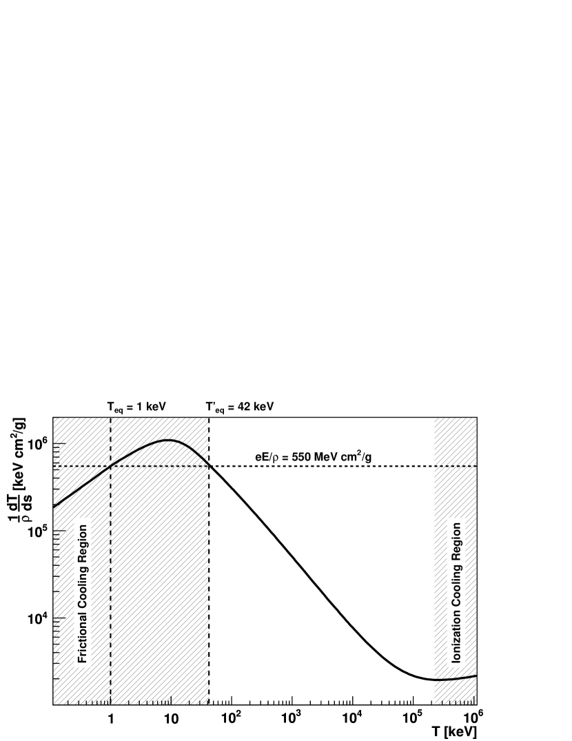
Figure 1: Stopping power (solid curve) of helium on $\upmu^{+}$. The horizontal dashed line shows the accelerating power of the restoring electric field for a particle of unit charge.

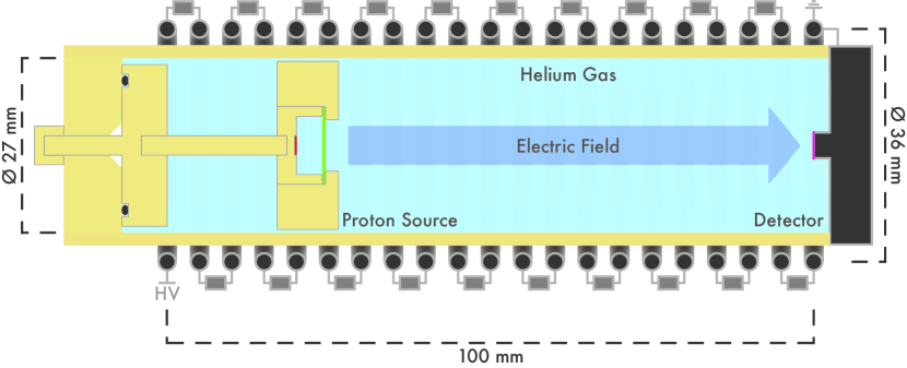
Figure 2: Scale diagram of the fcd cooling cell.

Frictional cooling involves the balancing of energy loss to a moderator with energy gain from an electric field to bring a beam of charged particles to an equilibrium energy and reduce dispersion. It requires the beam be in an energy region where the stopping power of the moderator medium—the energy loss per unit path length normalized by the medium density, $(1/\rho)\,\mathrm{d}T/\mathrm{d}s$—increases with increasing kinetic energy $T$. There are two energy regions where this requirement is met (figure 1). Ionization cooling schemes utilize particle beams in the high energy region [10]. Frictional cooling utilizes particle beams in the low energy region.

Applying an electric field to restore energy loss creates two equilibrium energies: a stable one at an energy $T_{\mathrm{eq}}$ below the ionization peak of the stopping power curve, where the energy loss per unit path length $\mathrm{d}T/\mathrm{d}s\propto\sqrt{T}$, and an unstable one at an energy $T_{\mathrm{eq}}^{\prime}$ above the peak, where $\mathrm{d}T/\mathrm{d}s$ decreases with increasing kinetic energy. Particles with kinetic energies below $T_{\mathrm{eq}}$ accelerate; those with kinetic energies between $T_{\mathrm{eq}}$ and $T_{\mathrm{eq}}^{\prime}$ decelerate. The coolable energy region is defined by $T<T_{\mathrm{eq}}^{\prime}$. Additionally, restoring lost energy only in the longitudinal direction provides transverse cooling.

For a chosen equilibrium energy, the electric field strength required to balance the energy loss scales directly with the density of the moderator. The density of the moderator must therefore be low, to keep the electric field strength within a feasible range. Helium and hydrogen gasses are good moderators because they have low densities and suppress the capture of electrons by the cooled particles [11] and the capture of the particles by the medium atoms [12] .

3 Frictional Cooling Demonstration Experiment

The fcd experiment at the mpp is designed to verify the working principles behind frictional cooling and the modeling of frictional cooling used in the simulation. The dependence of $T_{\mathrm{eq}}$ on moderator density and electric field strength can be measured and compared to monte carlo simulations.

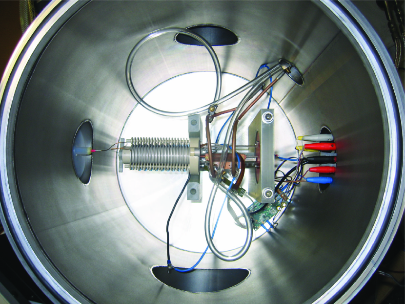
Figure 3: Photo of the experimental setup: visible are the gas cell (center) with the source on the left-hand side and detector on the right-hand side; the connection to hv (left); electronics feedthroughs (right) leading to the electronics (bottom right); and the gas feedthroughs (top right).

The experiment consists of a gas cell mounted inside an accelerating grid that provides the restoring electric field (figure 2). A proton source and an open silicon drift detector (sdd) are mounted inside the gas cell. The whole construction is then placed inside a vacuum tank (figure 3).

The accelerating grid is constructed from twenty-one metal rings, $3\text{\,}\mathrm{mm}$ thick, spaced $5\text{\,}\mathrm{mm}$ apart, connected in series with $64\text{\,}\mathrm{M\SIUnitSymbolOhm}$ resistors between rings. The rings enclose a cylindrical space $33\text{\,}\mathrm{mm}$ in diameter and $100\text{\,}\mathrm{mm}$ long from the center of the first ring to the center of the last ring. The first ring is connected to a power supply capable of providing voltages up to $100\text{\,}\mathrm{kV}$; the last ring is grounded. The central axis of the grid defines the $z$ direction, with $z\,=\,$0\text{\,}\mathrm{mm}$$ at the center of the high-voltage (hv) ring and $z\,=\,$100\text{\,}\mathrm{mm}$$ at the center of the ground ring. The grid creates a nearly uniform electric field along $z$ with strengths up to $1\text{\,}\mathrm{MV}\text{\,}{\mathrm{m}}^{-1}$ (see section 3.1).

The gas cell is a cylinder made of peek, with an outer radius of $31\text{\,}\mathrm{mm}$ and inner radius of $27\text{\,}\mathrm{mm}$. It is centered inside the accelerating grid. The end of the cell nearest the hv ring is sealed but for a small hole on the $z$ axis through which the proton source is mounted. The end of the cell nearest the ground ring is sealed by a grounded metal flange that holds the sdd and provides gas input and output feedthroughs.

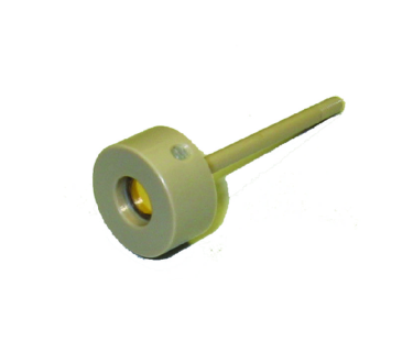
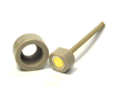
Figure 4: Photo of the proton source assembled (left) and disassembled (right). The gold-colored disc is the americium. The cylindrical cap holds the mylar foil.

The proton source (figure 4) consists of an open alpha source covered with a Mylar foil. The alpha particles free protons from the Mylar (see section 3.2). The source is embedded in the top of a lollipop made of peek. A cap that fastens to the lollipop head holds the Mylar foil in place. Foils of various thicknesses can be swapped into the construction easily and quickly.

The lollipop stick screws into the head at one end and into a cylindrical platform on the opposite end. This platform is $25\text{\,}\mathrm{mm}$ in diameter. The platform with the attached lollipop fastens to the hv end of the gas cell forming a gas-tight seal.

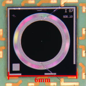
Figure 5: Photo of the sdd. The inner black circle is the back surface of the active region.

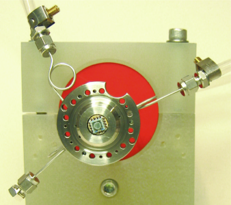
Figure 6: Photo of the sdd mounted into the gas feedthrough flange.

The sdd (figure 6) mounts through the gas feedthrough flange (figure 6) to a peek holder; when fastened tightly, this mounting provides a gas-tight seal. The peek holder also acts as an electronics feedthrough for the sdd. This construction allows for a quick exchange of the sdd.

3.1 Electric Field

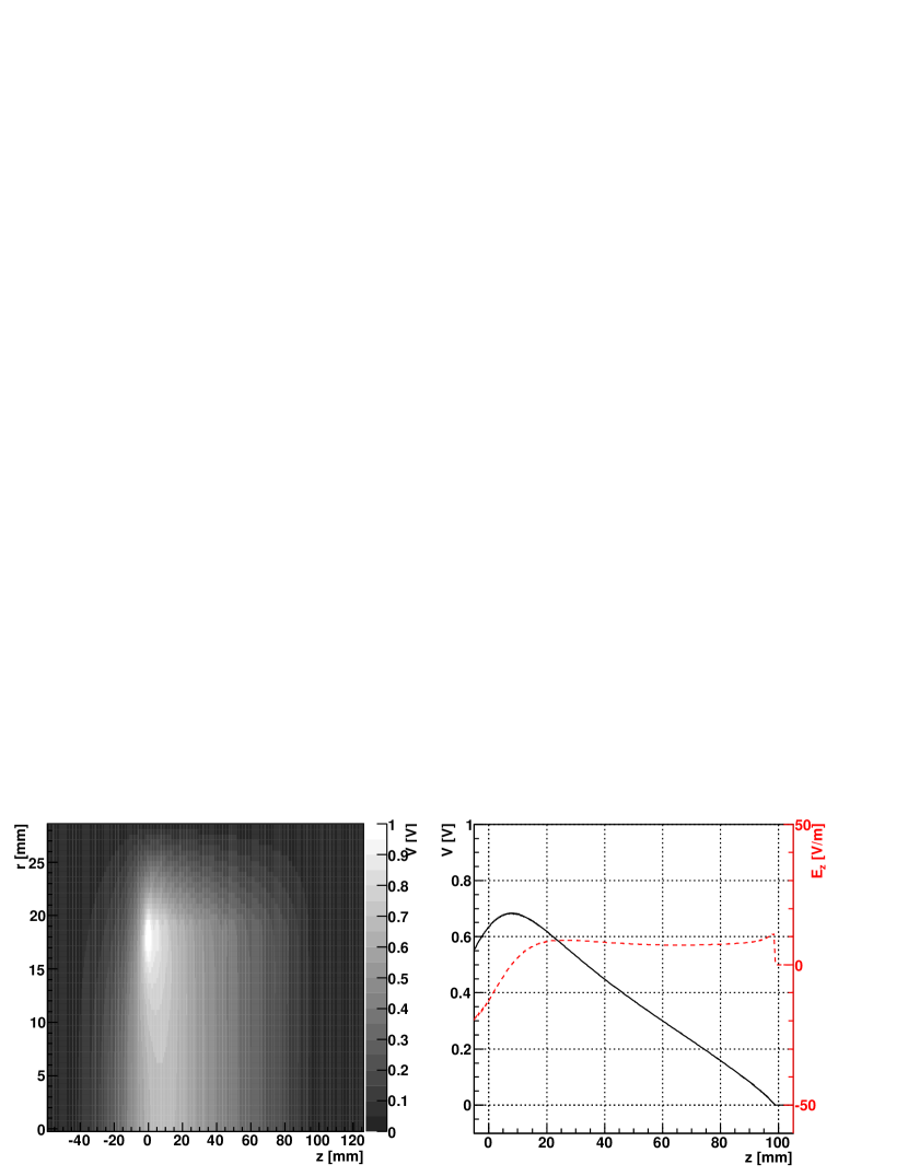
Figure 7: Map of the potential, for a voltage of $1\text{\,}\mathrm{V}$ applied to the first ring, in the $z$–$r$ plane (left) and the potential (black; left axis) and longitudinal electric field strength (dashed; right axis) on the $z$ axis (right) created by the accelerating grid (with plastic source holder).

A map of the electric field created by the accelerating grid is needed for the full simulation of the fcd experiment (section 4) as well as for characterizing the detector’s response to protons (section 5.2). We use a successive overrelaxation algorithm to calculate the electric field (figure 7). This calculation revealed that the potential is at its maximum not at $z=$0\text{\,}\mathrm{mm}$$, but instead at $z=$9\text{\,}\mathrm{mm}$$. Therefore the surface of the proton source must be placed at $z>$9\text{\,}\mathrm{mm}$$. The electric field is strongest and also nearest to uniform at $z>$20\text{\,}\mathrm{mm}$$. In the simulation of the fcd cell and in the experimental setup for the measurement of proton spectra, the source surface is therefore placed at $z=$20\text{\,}\mathrm{mm}$$.

3.2 Proton Source

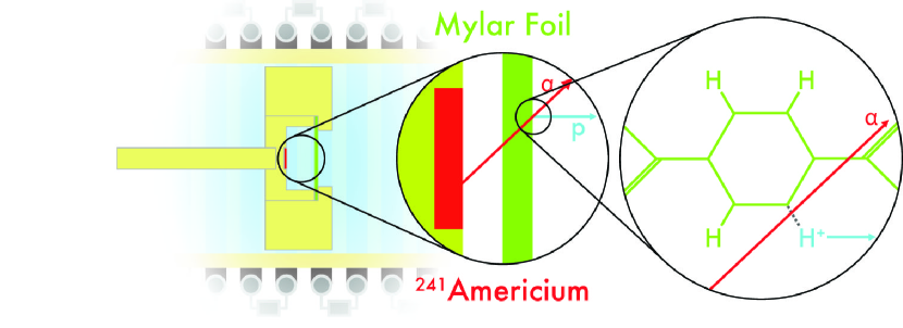
Figure 8: Schematic of the proton production mechanism

Energy ( M eV )	5.388	5.422	5.485
Branching Ratio (%)	1.0	13.0	84.5

Table 1: Energies and branching ratios (BR) for alpha particles emitted by ${}^{241}{\rm Am}$ with branching ratio greater than 0.4%

The proton source contains a $74\text{\,}\mathrm{kBq}$ ${}^{241}{\rm Am}$ alpha source covered by a thin Mylar foil. The americium emits alpha particles with energies approximately $5\text{\,}\mathrm{MeV}$ (table 1). As they pass through the Mylar, they break carbon–hydrogen bonds, freeing hydrogen nuclei from the Mylar molecule (figure 8). When these bonds are broken near the outer surface of the foil, the electric field can accelerate the resultant protons out of the foil before they are recaptured.

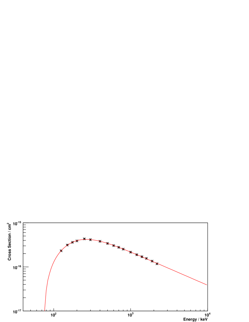
Figure 9: Experimentally measured cross section for the ionization of molecular hydrogen by He²⁺ [13] (points) and a fit adapted from [14] (line)

The number of bonds an $\upalpha$ breaks per unit distance is $n_{\mathrm{p}}$(E) = $\sigma_{\mathrm{ion}}$(E)⋅$\rho_{\mathrm{H}}$, where $\sigma_{\mathrm{ion}}$ is the cross section for ionization of molecular hydrogen by He²⁺ and $\rho_{\mathrm{H}}$ is the concentration of hydrogen in Mylar, $34.35\text{\,}\mathrm{n}\mathrm{m}\rpcubed$. The measured cross section for ionization of molecular hydrogren,

$$\textrm{He}^{2+}+\textrm{H}_{2}\to\textrm{He}^{n}+\textrm{p},$$

where Heⁿ is any charge state of helium, was reported in [13]. To describe the cross section (figure 9), we fit to the data a semi-empirical formula for the cross section of hydrogen on helium found in [14],

$$\sigma=\sigma_{0}\cdot a_{1}\,\left(\frac{E^{\prime}}{E_{R}}\right)^{\displaystyle a_{2}}{\Bigg{/}}\left(1+\left(\frac{E^{\prime}}{a_{3}}\right)^{\displaystyle a_{2}+a_{4}}+\left(\frac{E^{\prime}}{a_{5}}\right)^{\displaystyle a_{2}+a_{6}}\right),$$

where $E^{\prime}=E-E_{t}$ is the energy of the $\upalpha$ minus the threshold energy of the process, $E_{t}$; $E_{R}$ is the Rydberg energy multiplied by $m_{\mathrm{He}}/m_{\mathrm{e}}$. The $a_{i}$ are the fit parameters, and $\sigma_{0}$ is a scaling factor equal to $\power{10}{-16}\text{\,}{\mathrm{cm}}^{2}$.

The americium is in the form of a disc $2.5\text{\,}\mathrm{mm}$ in diameter, which is embedded in a plastic lollipop-shaped holder. It is completely open on its exposed side. A cap fits over the lollipop to hold the Mylar foil in place at a distance of $2.45\text{\,}\mathrm{mm}$ from the source. The cap has a circular opening $3.5\text{\,}\mathrm{mm}$ in diameter centered over the source.

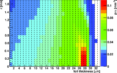
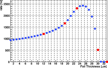
Figure 10: Radial distribution of p/$\upalpha$ (left) and total proton production rate for a $74\text{\,}\mathrm{kBq}$ alpha source (right) as functions of Mylar foil thickness. Both rates count only protons produced in the last $1\text{\,}\mathrm{nm}$ of foil.

We simulated this proton source in Geant4 [15]. The americium emits alpha particles isotropically. We tracked those alpha particles that pass through the foil and record their trajectories and energy losses in the Mylar foil. We calculate the number of C–H bonds broken by an $\upalpha$ at a point along its trajectory using its Geant4-calculated energy. This is used to calculate the radial distribution (in a plane parallel to the surface of the foil) of the number of C–H bonds broken within the last 1- n m as a function of thickness of the foil traversed. We used $1\text{\,}\mathrm{nm}$ as an estimate of the depth from which a proton can escape out of the foil because this is roughtly the size of the Mylar monomer. Figure 10 (left) displays the results for thickness of the foil from $1\text{\,}\mathrm{\SIUnitSymbolMicro m}$ to $33\text{\,}\mathrm{\SIUnitSymbolMicro m}$ in $1\text{\,}\mathrm{\SIUnitSymbolMicro m}$ steps; this is the precision on the thickness at which such foils are manufactured.

We also calculated the total proton production (again in the last $1\text{\,}\mathrm{nm}$) as a function of thickness of the Mylar foil (figure 10, right). The shape of the rate–thickness relationship is similar to that of the Bragg peak for $\upalpha$’s in Mylar; however, it is broadened by the distribution of the incidence angles of the $\upalpha$’s. The rate is maximum in the region of $23\text{\,}\mathrm{\SIUnitSymbolMicro m}$ and is zero above $30\text{\,}\mathrm{\SIUnitSymbolMicro m}$, since the $\upalpha$’s are stopped in the foil before reaching the surface. Around the rate-maximizing thickness, the proton production is spatially uniform, and at larger thicknesses, the protons are produced mainly at the center of the foil surface (figure 10). Though at the larger thicknesses the total rate is lower, when detector acceptance is taken into account (see section 20), the centralized proton production may be beneficial. The square-shaped markers in the right plot of figure 10 indicate the five thicknesses available for the experiment: 12, 19, 24, 30, and $33\text{\,}\mathrm{\SIUnitSymbolMicro m}$. By sandwiching foils together, we are also able to test a thickness of $31\text{\,}\mathrm{\SIUnitSymbolMicro m}$.

3.3 Silicon Drift Detector

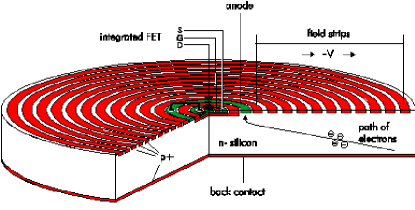
Figure 11: Schematic of the sdd from [16], showing the electrode structure used to deplete the detector bulk and setup the charge-collection field, and the fet.

The sdd, designed and constructed by the mpp’s Semiconductor Laboratory, measures particle energies in the range $100s\text{\,}\mathrm{e}\mathrm{V}$ to approximately $150\text{\,}\mathrm{keV}$ . The detector is constructed on an n-type silicon wafer $450\text{\,}\mathrm{\SIUnitSymbolMicro m}$ thick. The exposed (back) surface of the detector is covered uniformally with a 30- n m -thick aluminum electrode. The opposite surface is implanted with concentric rings of p-type silicon (figure 11). A negative potential (on the order of $-100\text{\,}\mathrm{V}$) on the aluminum depletes the silicon. The p-type rings are placed at voltages that produce a well-shaped potential inside the silicon. Ionizing particles produce a number of electron-hole pairs in the silicon in proportion to the amount of energy they deposit along their trajectory; the electrons then drift to the center of the p-doped surface of the detector, where a field-effect transistor produces a signal.

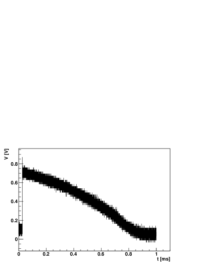
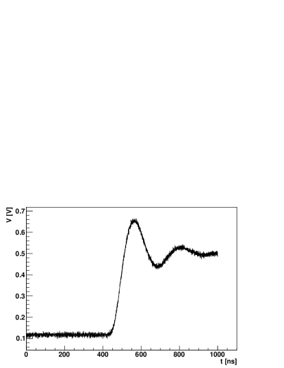
Figure 12: Signal from sdd after initial amplification. The plot on the right shows the rising edge of the signal, shown in full on the left.

The voltages for depletion of the silicon and setting up of the potential well are regulated by electronics manufactured by PNSensor [17]. The detector outputs a saw-tooth-shaped voltage pulse that after initial amplification by these electronics has a rise time of 30 to 40  n s  (figure 12) and an amplitude $V_{\mathrm{det}}~{}\!\approx~{}\!($1.2\text{\,}\mathrm{mV}\text{\,}{\mathrm{keV}}^{-1}$)\;T_{\mathrm{dep}}$, where $T_{\mathrm{dep}}$ is the energy the particle deposits in the active layers of the detector.

3.4 Electronic Readout

Figure 13: Shaped and digitized signal from the sdd with pedestal and peak fits.

Figure 14: Saturated signal from the sdd.

A shaping amplifier with a shaping time of $0.25\text{\,}\mathrm{\SIUnitSymbolMicro s}$ converts this quick signal to a fin-shaped pulse 3 to 4  µ s  wide (figure 14). The shaper preserves the linearity of the signal amplitude’s dependence on $T_{\mathrm{dep}}$. The signal is split in two: one part is used for triggering; the other is digitized and saved for offline analysis.

A 12-bit adc from National Instruments [18], interfaced with a computer via LabView [19], digitizes the signal with a sampling rate of $10\text{\,}\mathrm{MHz}$. Before entering the adc, the signal is delayed $4.75\text{\,}\mathrm{\SIUnitSymbolMicro s}$ with respect to the trigger signal, so that the baseline voltage before the signal is recorded as well. The adc records the event for $10\text{\,}\mathrm{\SIUnitSymbolMicro s}$ (100 samples).

A window discriminator, consisting of two trailing-edge constant fraction discriminators (cfd), one setting a low threshold, the other a high threshold, produces the trigger signal for the adc to begin sampling. The low-threshold cfd filters out low-amplitude voltage fluctuations—that is, noise. Since the adc has a maximum triggering rate of $30\text{\,}\mathrm{Hz}$, when needed, the high-threshold cfd was used to filter out unimportant signals that had large amplitudes, namely those from $\upalpha$ particles.

A particle that deposits too much energy in the detector produces a charge-saturated signal (figure 14). The signal is distorted and the energy of the particle cannot be reconstructed. These signals themselves are filtered out by the window discriminator; however, the saturation often produces secondary signal peaks in the trailing edge of the original signal. These peaks are large enough to pass the low-threshold cfd but small enough for the high-threshold cfd to not veto them. To prevent these signals from swamping the adc, a gate generator can produce a veto signal from the high-threshold cfd’s trigger pulse. The length of the gate can be set within a large range of times from less than $100\text{\,}\mathrm{ns}$ to greater than $11\text{\,}\mathrm{s}$.

3.5 Offline Analysis

The amplitude of a signal above the baseline linearly corresponds to the energy deposited in the detector by the incoming particle. The shape of the signal around its peak is approximately gaussian. However, since outside this region the signal is not perfectly gaussian, we cannot fit the whole signal with a gaussian shape plus a pedestal to get both the amplitude and the baseline. Instead, we fit the peak and the samples before the signal separately (figure 14). Fitting the first approximately $2\text{\,}\mathrm{\SIUnitSymbolMicro s}$ with a constant pedestal plus a gaussian function that describes the start of the signal gives the baseline value. Fitting a symmetric $2\text{\,}\mathrm{\SIUnitSymbolMicro s}$ window around the peak with a gaussian function gives the signal amplitude.

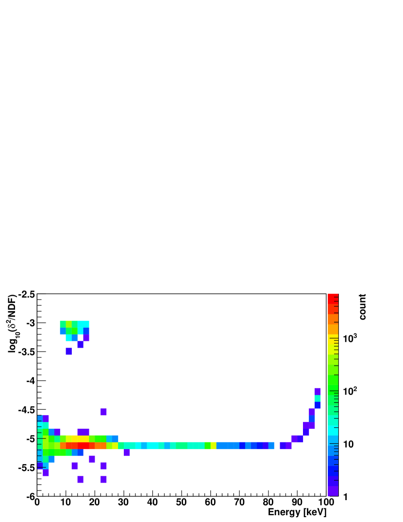
Figure 15: $\chi^{2}/$NDF distributions as a function of event energy for a background run.

A visual investigation of the pulses revealed two different classes of signal: one that contained one peak, which the functional form reproduced well; and one that contained multiple peaks, which the functional form did not reproduce well. The poorly fitted pulses were clearly due to noise. Cutting on $\log(\delta^{2})<-4$ (figure 15), defined by

$$\delta^{2}=h^{-2}\sum_{i}[V_{i}-f(t_{i})]^{2},$$

rejects such noise, where $V_{i}$ and $t_{i}$ are the voltage and time of the $i$th voltage sample, $f(t_{i})$ is the fitted voltage at time $t_{i}$, and $h$ is the maximum voltage of the event.

3.6 Detector Calibration

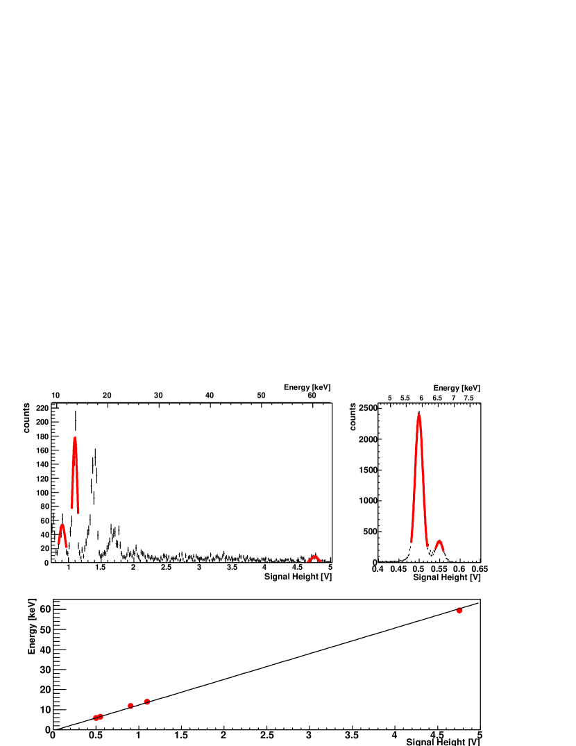
Figure 16: ${}^{241}{\rm Am}$ (top left) and ${}^{55}{\rm Fe}$ (top right) x-ray spectra, and calibration fit (bottom).

To calibrate the detector and readout system, we record the spectra of the known x-ray sources ${}^{55}{\rm Fe}$ and ${}^{241}{\rm Am}$. The two sources provide x-rays at many energies between $5\text{\,}\mathrm{keV}$ and $60\text{\,}\mathrm{keV}$, allowing us to learn the proportionality of the detectors signal amplitude to $T_{\mathrm{dep}}$ (figure 16) and to check the linearity of the detector response.

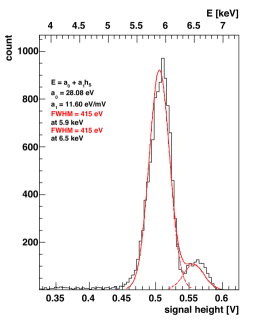
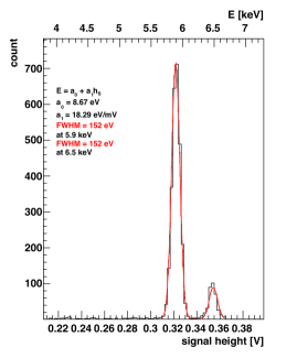
Figure 17: ${}^{55}{\rm Fe}$ spectra taken with the sdd at room temperature (left) and cooled to $-20\text{\,}\mathrm{\SIUnitSymbolCelsius}$ (right).

Since x-rays deposit their energy locally and uniformally inside the silicon, these sources also allow us to measure the energy resolution of the detector and our read-out system without influences from any dead layer structure. The resolution, here defined as the fwhm of an energy peak, is greatly affected by the temperature of the detector (figure 17). At room temperature, the detector has resolutions at the Mn K$\upalpha$ line of ${}^{55}{\rm Fe}$ ($5.9\text{\,}\mathrm{keV}$) greater than $400\text{\,}\mathrm{eV}$. When cooled to temperatures below $0\text{\,}\mathrm{\SIUnitSymbolCelsius}$, the detector reaches resolutions below $150\text{\,}\mathrm{eV}$.

3.7 Gas Purity

The frictional cooling effect and the operation of the open sdd require that the moderating gas be uncontaminated.

The detector has a dead layer of $30\text{\,}\mathrm{nm}$ of aluminum on top of the silicon that forms its active volume. As well, in the first approximately $200\text{\,}\mathrm{nm}$ of the silicon, the detector has a charge collection efficiency below 100%. In the energy range of interest, $T\lessapprox$30\text{\,}\mathrm{keV}$$, protons deposit a significant amount of energy in the aluminum and deposit their remaining energy largely in the region of reduced collection efficiency. Therefore, the sdd measures only 35% to 65% of the proton’s energy (section 5.2).

Impurities in the gas environment can build up on the detector’s surface, which is the coldest surface in the experiment setup, increasing the amount of material that protons must traverse before entering the active layers of the detector. Even a thin layer of built-up gas impurities significantly reduces the amount of energy measured and, due to straggling in the trajectories of protons through the dead layers, greatly reduces the detector’s energy resolution. The main sources of impurities are outgassing of molecules from the plastic pieces in the experiment construction and contamination of the gas from impurities either in the gas source or entering along the gas transfer line. The effects of outgassing can be greatly reduced by pumping the gas cell down to a low pressure ($\power{10}{-6}\text{\,}\mathrm{m}\bbar$) for several days. During this time, the plastic pieces expel foreign molecules, leaving the environment cleaner for data-taking runs.

The boil-off from cryogenic liquids is used as an ultrapure gas source. The gas transfer lines are tightly sealed, capable of holding pressures down to $\power{10}{-9}\text{\,}\mathrm{m}\bbar$, to prevent air leaking into the gas. As well, the transfer lines are entirely constructed from stainless steel, so no outgassing can contaminate the gas on the way from the source to the cell. The construction of an impurity trap, improvements in the gas line, and ultrapure helium sources will be implemented for running he full system.

3.8 Electric Breakdown

Due to the large electric field strengths it provides, the accelerating grid must be kept in high vacuum ($P<$\power{10}{-4}\text{\,}\mathrm{m}\bbar$$) in order to prevent breakdown of the electric field between grid rings. Even at high vacuum, breakdowns can occur if the lines carrying the high voltage come too near to lower voltage rings or grounded pieces. Such breakdowns were observed in early versions of the experiment construction in which the high voltage was lead to the hv ring by an insulated wire that passed along the length of he accelerating grid. Electrical discharges originated at the hv ring and traveled down the surface of the wire’s insulation to the grounded detector flange, when high voltages as low as $15\text{\,}\mathrm{kV}$ were applied to the hv ring. To prevent this from occuring, the construction was altered to bring high voltages to the hv ring from the opposite side (figure 3)

The gas seal at the source side of the cell must be very tight since it is at the hv end of the grid. A small leak can stream gas over the rings creating a path for the breakdown between rings. It can also provide a path for charge to flow in a breakdown from inside the gas cell to the hv ring. Both breakdowns mechanisms were observed in an early version of the experiment construction in which the proton source was mounted directly through the gas cell wall. This construction did not create a tight enough gas seal, and breakdowns were observed at gas pressures above several $\power{10}{-1}\text{\,}\mathrm{m}\bbar$, when high voltages as low as $10\text{\,}\mathrm{kV}$ were applied to the hv ring. To prevent gas leaks causing such breakdowns, we constructed the source-holder platform described above.

3.8.1 Breakdown Inside the Gas Cell

Breakdown of the electric field also occurs entirely inside the gas cell. This can be particularly dangerous since a breakdown that strikes the detector can destroy it or the detector electronics. The frequency and strength of these breakdowns depends greatly on the source-holder platform.

We constructed two platforms: one made of peek that does not alter the electric field of the accelerating grid; and one made of stainless steel that can be connected to the hv ring or left unconnected (floating), and alters the shape of the electric field at the hv end.

When the metal platform is electrically connected to the hv ring, such a large current is drawn at any pressure that the high voltage supply is incapable of providing enough current to hold a hv above $1\text{\,}\mathrm{kV}$. However, when the platform is left floating, higher voltages can be reached before a breakdown from the platform to a point inside the gas cell occurs.

Figure 18: Threshold voltage for breakdown of the electric field inside the gas cell for helium, nitrogen, and argon with a floating metal source-holder platform.

A photodiode, mounted onto an empty sdd housing that was mounted inside the gas cell in place of the detector, measured the light from discharges in the gas allowing for measurement of the frequency of electric breakdown. We observed that disharges of a harmless size occured frequently ($\gtrapprox 1\text{\,}\mathrm{Hz}$), but did not drain enough current to alter the voltage. However, above a voltage threshold that depends on the pressure of the gas in the cell, we observed large discharges occuring with higher frequency. These discharges prevented the high voltage supply from keeping a constant voltage. The dependence of the threshold voltage $V_{\mathrm{br}}$ on gas pressure $p$ (figure 18) matches the predictions from the Townsend discharge theory [20] augmented by an offset voltage $V_{0}$,

$$V_{\mathrm{br}}=\frac{Bpd}{\ln(Apd)-\ln(\ln(1+\gamma^{-1}))}+V_{0},$$ (1)

where $d$ is the distance over which the discharge takes place, $A$ and $B$ are the Townsend coefficients, and $\gamma$ is the secondary emission coefficient. Coefficients $A$, $B$, and $\gamma$ are different for each gas. Fitting the Townsend theory to the voltage-threshold data with $d$ and $V_{0}$ as the only free parameters indicates a discharge distance on the order of c m , the same order of size as the gas cell.

Tests conducted with the peek platform and americium source indicate that charge freed from the gas by the americium alphas builds up on the platform until a breakdown occurs from the platform to the hv ring. These breakdowns create large discharges and are fatal to the detector and detector electronics. However, these breakdowns do not occur when the seal between the peek platform and the end of the gas cell is made very gas tight, closing the path for charge to take during a breakdown. In the gas-tight cell, electric fields of strengths up to $650\text{\,}\mathrm{kV}\text{\,}{\mathrm{m}}^{-1}$ have been reached without breakdown at gas pressures from $\power{10}{-7}\text{\,}\mathrm{m}\bbar$ to $1.25\text{\,}\bbar$.

4 FCD Cell Simulation

We simulated the frictional cooling process in the fcd cell to provide expectations for proton energy spectra under different configurations. For this simulation as well as full frictional cooling schemes [21, 22], we developed software based on Geant4, called CoolSim [23]. It implements the low-energy packages of Geant4 optimized for the tracking of protons and muons through matter. As well, we have added new processes to the Geant4 framework for the simulation of charge exchange processes at low energies in gaseous materials [21].

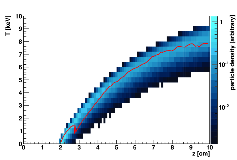
Figure 19: Simulated kinetic energy distributions of protons (shaded) and the kinetic energy of a single proton (line) as a function of $z$ in the fcd cooling cell filled with helium gas at $40\text{\,}\mathrm{m}\bbar$ and an electric field strength of $0.4\text{\,}\mathrm{MV}\text{\,}{\mathrm{m}}^{-1}$.

The cell simulated was exactly as described in section 3, with the electric field shape as calculated in section 3.1. The protons were simulated as originating from a point source located on the $z$ axis at the center of the 5th ring ($z=$20\text{\,}\mathrm{mm}$$). In the following discussion all data are taken from runs in which ten thousand protons were simulated for each of the combinations of nine electric field strengths, evenly spaced between $0.1\text{\,}\mathrm{MV}\text{\,}{\mathrm{m}}^{-1}$ and $0.5\text{\,}\mathrm{MV}\text{\,}{\mathrm{m}}^{-1}$, and nine helium gas densities, logarithmically spaced between $1\text{\,}\mathrm{m}\bbar$ and $700\text{\,}\mathrm{m}\bbar$. In each simulation run, protons start at rest and accelerate through the gas in the positive $z$ direction, approaching the equilibrium energy (figure 19).

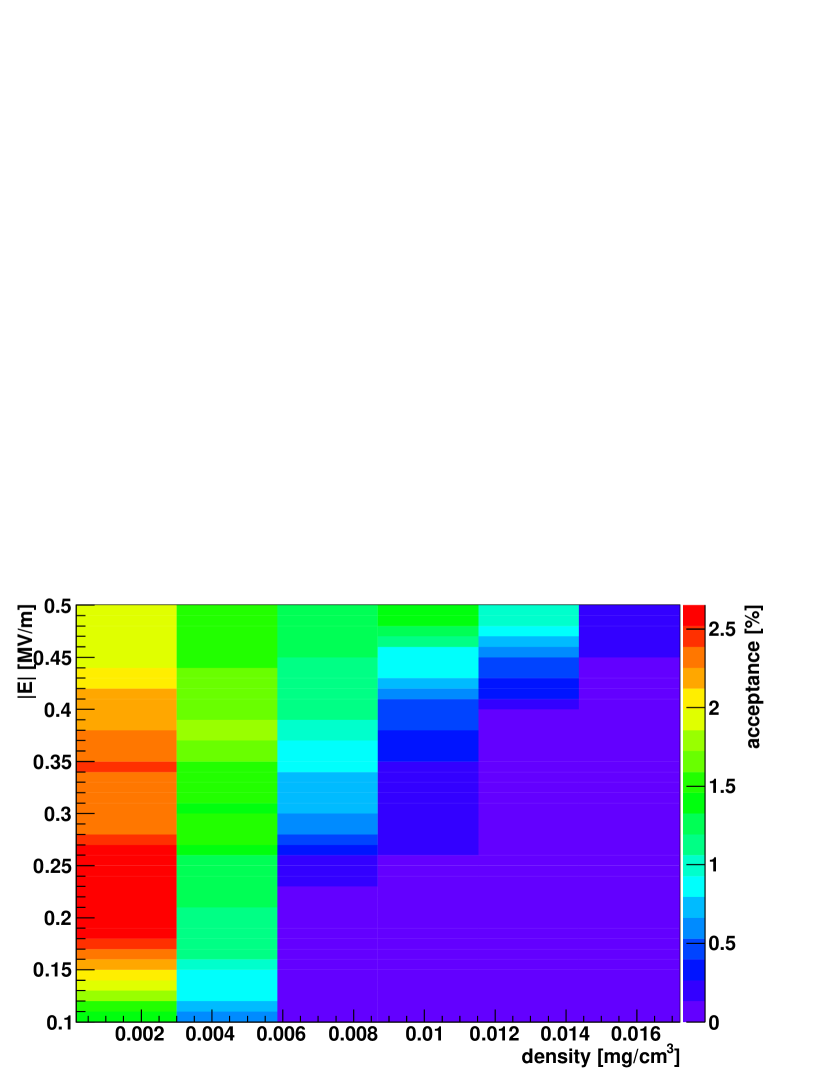
Figure 20: Simulated detector acceptance as a function of electric field strength and helium gas density.

As they accelerate, they interact with the helium gas, scattering away from the $z$ axis and decreasing acceptance in the sdd (figure 20), which has a radius of $1.78\text{\,}\mathrm{mm}$. The mean free path for scattering decreases with increasing helium gas pressure, causing more muons to scatter away from the sdd at higher pressures. However, the stronger electric fields refocus some of those scattered protons towards the $z$ axis. The lowest acceptances are expected for the high-pressure–weak-field region of the parameter space. The scattering can be seen in the highlighted trajectory of figure 19: after scattering into a direction opposed to the electric field, the proton decelerates, turns around, and then reaccelerates. This produces the abrupt kinetic energy fluctuation seen in the figure.

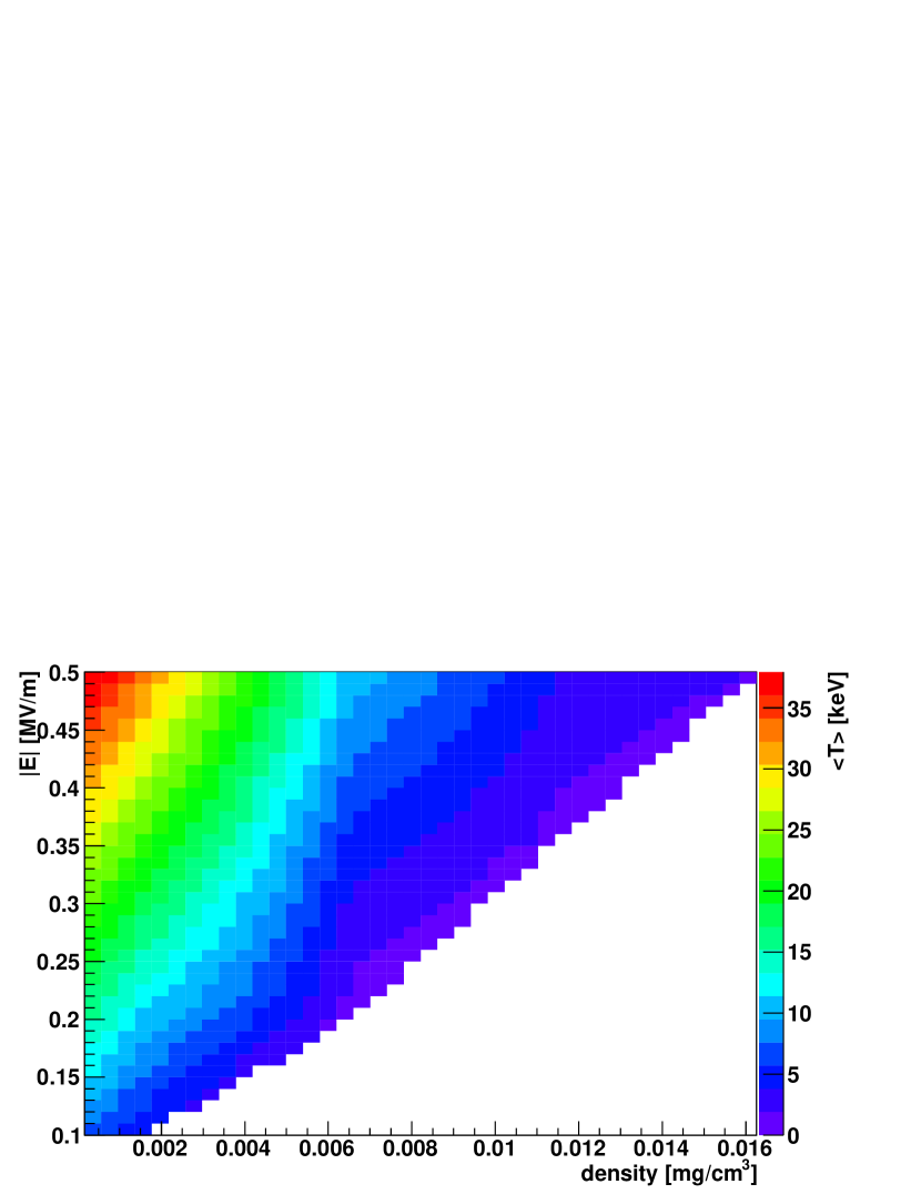
Figure 21: Simulated mean kinetic energy of protons at the sdd as a function of electric field strength and helium gas density.

For each combination of electric field strength and gas pressure the mean of the kinetic energy distribution at the sdd ($z=$10\text{\,}\mathrm{cm}$$, $r<=$1.78\text{\,}\mathrm{mm}$$) is calculated (figure 21). For a fixed electric field strength, raising the gas pressure increases the energy loss to the helium, decreasing the mean energy at the detector. For a fixed gas pressure, raising the electric field strength increases the restorative energy gain, increasing the mean energy. Both behaviors are as expected from figure 1.

5 Measurements

Several measurements were made using the experimental setup to calibrate the detectors (section 3.6) and measure the effect of their dead layers, as well as to measure the x-ray background, and verify the production of protons. All of the following measurements were made with the proton source, with a $23$-$\mathrm{\SIUnitSymbolMicro}\mathrm{m}$-thick Mylar foil, mounted in the accelerating grid at $z=$20\text{\,}\mathrm{mm}$$ and the detector cooled to approximately $15\text{\,}\mathrm{\SIUnitSymbolCelsius}$. Background and gasless proton measurements were made without the gas cell in place. The total data taking rate was approximately $10\text{\,}\mathrm{Hz}$. The x-ray rate was approximately $1.5\text{\,}\mathrm{Hz}$; the proton rate was approximately $2\text{\,}\mathrm{Hz}$; and the remaining rate was due to saturated pulses from M eV  alpha particles.

5.1 Background

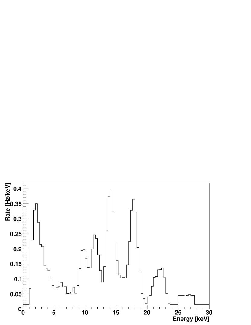
Figure 22: Background spectra with ${}^{241}{\rm Am}$ source present and the gas cell evacuated.

Energy		BR		D	BR⋅D
( k eV )		(%)		(%)	(%)
11.	87	0.	66	92	0.	61
13.	76	1.	07	81	0.	87
13.	95	9.	6	79	7.	6
15.	86	0.	15	62	0.	10
16.	11	0.	18	61	0.	11
16.	82	2.	5	58	1.	4
17.	06	1.	5	56	0.	8
17.	50	0.	65	54	0.	35
17.	99	1.	37	51	0.	70
20.	78	1.	39	36	0.	50
21.	10	0.	65	35	0.	23
21.	34	0.	59	35	0.	20
21.	49	0.	29	34	0.	10
26.	34	2.	40	23	0.	56
59.	54	35.	90	3	1.	21

Table 2: Energies, branching ratios (BR), detectability (D), and BR⋅D for x-rays emitted by ${}^{241}{\rm Am}$ with branching ratio greater than 0.2%

The ${}^{241}{\rm Am}$ in the proton source emits x-rays in the energy range of interest for the proton measurements ($E\lesssim$30\text{\,}\mathrm{keV}$$). The observed rate of x-rays is comparable to that of protons, so the background energy spectrum must be measured for subtraction from the proton energy spectra. The background spectrum (figure 22) contains several peaks from the ${}^{241}{\rm Am}$ spectrum (table 2) as well as low-amplitude noise. To reduce the low-amplitude noise rate, a voltage threshold corresponding to an energy threshold of $1\text{\,}\mathrm{keV}$ is used in data recording. The probability that the x-rays interact in the sdd, which is $450\text{\,}\mathrm{\SIUnitSymbolMicro m}$ thick, rapidly decreases with increasing energy in the range of interest. Table 2 lists the detectability (D), defined as the percentage of x-rays interacting in the sensitive volume of the detector, and detectable branching ratio (D⋅BR) for the prominent x-ray lines.

5.2 Proton Observations

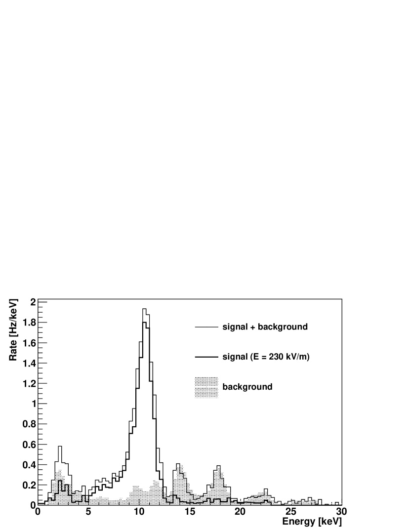
Figure 23: Energy spectrum for an $E=$23\text{\,}\mathrm{kV}\text{\,}{\mathrm{m}}^{-1}$$ run: full spectrum (line), background-removed spectrum (thick line), and background (highlighted).

Energy spectra were measured with electric field strengths evenly spaced from $70\text{\,}\mathrm{kV}\text{\,}{\mathrm{m}}^{-1}$ to $300\text{\,}\mathrm{kV}\text{\,}{\mathrm{m}}^{-1}$ in $10\text{\,}\mathrm{kV}\text{\,}{\mathrm{m}}^{-1}$ steps. The background spectrum ($E=$0\text{\,}\mathrm{kV}\text{\,}{\mathrm{m}}^{-1}$$) and proton spectra ($E>$0\text{\,}\mathrm{kV}\text{\,}{\mathrm{m}}^{-1}$$) were analyzed together to discover the overall background rate and the signal rate above that background for each spectrum. Figure 23 shows an example spectrum, for $E=$230\text{\,}\mathrm{kV}\text{\,}{\mathrm{m}}^{-1}$$. The background spectrum as calculated from all the measured spectra is shown for comparison. The spectrum has a prominent proton peak centered around approximately $11\text{\,}\mathrm{keV}$, which is lower than the $18.4\text{\,}\mathrm{keV}$ expected from the calculation of the electric field. The discrepancy is due to energy deposition in the dead and partially-inactive layers of the detector. The peak has a fwhm of approximately $2\text{\,}\mathrm{keV}$. This is larger than the x-ray energy resolution at the same energy, but is as expected from the distribution of proton energy loss in the dead layers.

The proton peak also has a tail to lower energies. This is due to protons striking the outer edges of the detector surface where they encounter larger dead layers. The increase in the low-energy noise above the background rate may be due to fluorescence of the silicon and aluminum of the detector, which produces peaks in this range.

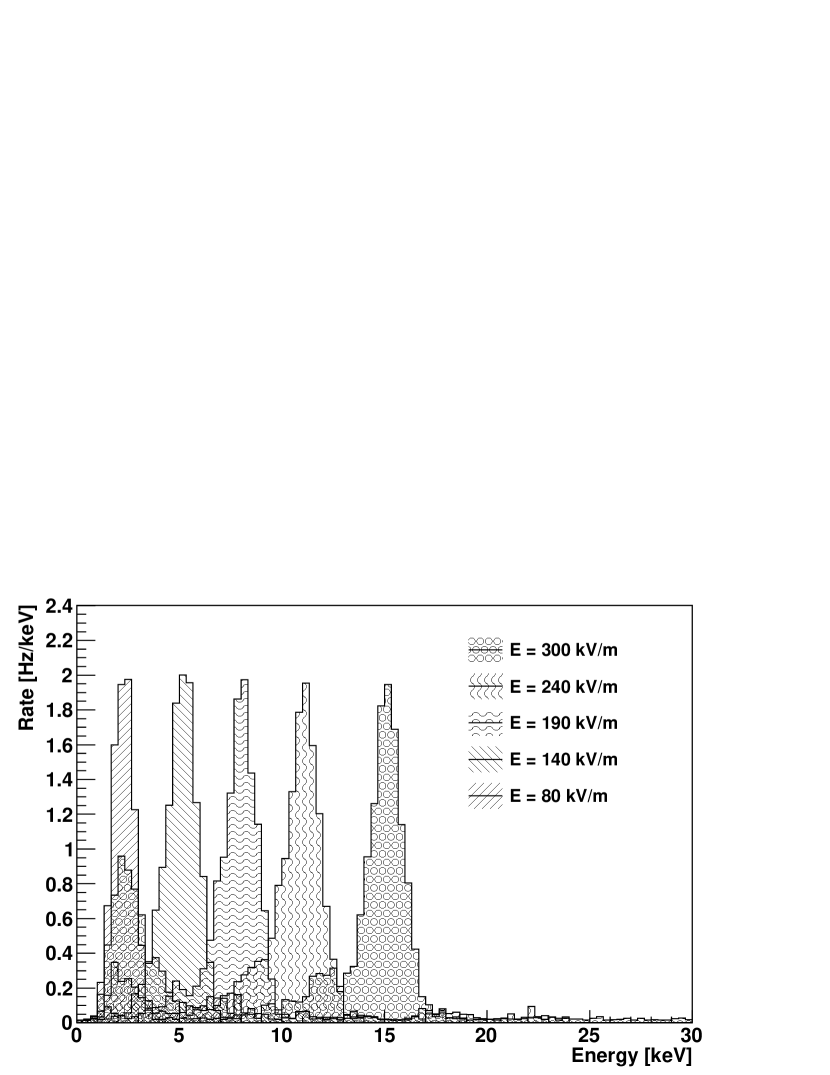
Figure 24: Proton energy spectra, with background removed, for five representative strengths of the electric field.

Figure 24 shows five of the proton spectra along with the overall background. The peak centers are evenly spaced in accordance with the field strengths at which they were measured. As well, the proton rate remained nearly constant with changing electric field strength.

Figure 25: sdd-measured energy as a function of expected proton energy (top) and the ratio of measured to expected energy as a function of expected energy (bottom).

The upper plot of figure 25 shows the peak centers of the spectra ($T_{\mathrm{meas}}$, obtained by fitting with a gaussian distribution) as a function of the expected proton energy ($T_{\mathrm{exp}}$), which is obtained from from the numerical calculation of the electric field. The detector’s dead layers are of a thickness on the order of 100s of n m , which is also the order of size of the penetration depth of k eV  protons. The higher-energy protons travel further into the detector, depositing a larger ratio of their energy in fully active layers of the detector (figure 25, bottom).

The lowest energy run in figure 25, for which $E=$70\text{\,}\mathrm{kV}\text{\,}{\mathrm{m}}^{-1}$$, has $T_{\mathrm{meas}}=$0\text{\,}\mathrm{keV}$$ because after depositing energy in the dead layers, the protons didn’t have enough energy left to be measureable above the low-energy threshold, which vetoes electronic noise in the detector readout system. Any further build up of a dead layer increases the minimum energy protons must have in order to be detectable.

6 Conclusion

The fcd experiment at the Max Planck Institute for Physics, Munich, has been commissioned to study the working principle behind frictional cooling. The experiment construction is complete and all parts have been commissioned: The accelerating grid can maintain electric field strengths without breakdown up to $900\text{\,}\mathrm{kV}\text{\,}{\mathrm{m}}^{-1}$ in an evacuated gas cell and up to $650\text{\,}\mathrm{kV}\text{\,}{\mathrm{m}}^{-1}$ in a pressurized gas cell with pressures up to $1.25\text{\,}\bbar$. The detector can measure energy with good resolutions and can be reliably operated in the strong field of the accelerating grid. The gas system is capable of maintaining a specified pressure for several hours. Proton spectra have been measured, demonstrating that the source functions. The next step in the fcd experiment is the taking of data with the gas cell filled.

References

- Ankenbrandt et al. [1999] C. M. Ankenbrandt, et al., Status of muon collider research and development and future plans, Phys. Rev. ST Accel. Beams 2 (1999) 081001.
- Barger [1998] V. Barger, Overview of physics at a muon collider (1998).
- Barger et al. [1995] V. Barger, M. S. Berger, J. F. Gunion, T. Han, s-channel higgs boson production at a muon-muon collider, Physics Review Letters 75 (1995) 1462–1465. Number 8.
- Barger et al. [1998] V. Barger, M. S. Berger, T. Han, Chargino mass determination at a muon collider (1998).
- Lykken [1998] J. D. Lykken, Sparticle masses from kinematic fitting at a muon collider (1998).
- Eichten et al. [1998] E. Eichten, K. Lane, J. Womersley, Narrow technihadron production at the first muon collider, Phys. Rev. Lett. 80 (1998) 5489–5492.
- Schellman [1998] H. Schellman, Deep inelastic scattering at a muon collider-neutrino physics, AIP Conference Proceedings 435 (1998) 166–176.
- Cheung [1998] K. Cheung, Muon-proton colliders: Leptoquarks and contact interactions (1998).
- Abramowicz et al. [2005] H. Abramowicz, A. Caldwell, R. Galea, S. Schlenstedt, A muon collider scheme based on frictional cooling, Nucl. Instrum. Meth. A546 (2005) 356–375.
- Neuffer [1983] D. Neuffer, Principles and applications of muon cooling, Part. Accel. 14 (1983) 75.
- Stambaugh et al. [1974] R. D. Stambaugh, et al., Muonium formation in noble gases and noble-gas mixtures, Phys. Rev. Lett. 33 (1974) 568–571.
- Cohen [2002] J. S. Cohen, Capture of negative muons and antiprotons by noble-gas atoms, Phys. Rev. A 65 (2002).
- Tawara et al. [1985] H. Tawara, T. Kato, Y. Nakai, Cross sections for electron capture and loss by positive ions in collisions with atomic and molecular hydrogen, Atomic Data and Nuclear Data Tables 32 (1985) 235 – 303.
- Green and McNeal [1971] A. E. S. Green, R. J. McNeal, Analytic cross sections for inelastic collisions of protons and Hydrogen atoms with atomic and molecular gases, J. Geophys. Res 76 (1971) 133–144.
- Agostinelli et al. [2003] S. Agostinelli, et al., GEANT4: A simulation toolkit, Nucl. Instrum. Meth. A506 (2003) 250–303.
- Simson et al. [2007] M. Simson, et al., Detection of low-energy protons using a silicon drift detector, 2007. TU Munich.
- PNSensor [2010] PNSensor, http://www.pnsensor.de, 2010.
- National Instruments [2010] National Instruments, http://www.ni.com, 2010.
- LabView [2010] LabView, http://www.ni.com/labview, 2010.
- Pejovic et al. [2002] M. M. Pejovic, G. S. Ristic, J. P. Karamarkovic, Electrical breakdown in low pressure gases, Journal of Physics D: Applied Physics 35 (2002) R91.
- Greenwald et al. [2010] D. Greenwald, Y. Bao, A. Caldwell, Frictional cooling scheme for use in a muon collider, volume 1222, AIP, 2010, pp. 293–297.
- Bao et al. [2010] Y. Bao, A. Caldwell, D. Greenwald, G. Xia, Low-energy via frictional cooling, Nuclear Instruments and Methods in Physics Research Section A: Accelerators, Spectrometers, Detectors and Associated Equipment 622 (2010) 28 – 34.
- CoolSim [2010] CoolSim, http://wwwmu.mppmu.mpg.de/coolsim, 2010.